Article

Design and Scaling of Exoskeleton Power Units Considering Load Cycles of Humans

1
Institute of Electrical Energy Conversion, University of Stuttgart, 70569 Stuttgart, Germany
2
Institute of Modelling and Simulation of Biomechanical Systems, University of Stuttgart, 70569 Stuttgart, Germany
*
Author to whom correspondence should be addressed.
Robotics 2022, 11(5), 107; https://doi.org/10.3390/robotics11050107
Submission received: 25 August 2022 / Revised: 26 September 2022 / Accepted: 29 September 2022 / Published: 8 October 2022
(This article belongs to the Special Issue Mechatronics Systems and Robots)

Abstract

:
Exoskeletons are powerful tools for aiding humans with pathological conditions, in dangerous environments or in manually exhausting tasks. Typically, they are designed for specific maximum scenarios without taking into account the diversity of tasks and the individuality of the user. To address this discrepancy, a framework was developed for personalizing an exoskeleton by scaling the components, especially the electrical machine, based on different simulated human muscle forces. The main idea was to scale a numerical arm model based on body mass and height to predict different movements representing both manual labor and daily activities. The predicted torques necessary to produce these movements were then used to generate a load/performance cycle for the power unit design. Considering these torques, main operation points of this load cycle were defined and a reference power unit was scaled and optimized. Therefore, a scalability model for an electrical machine is introduced. This individual adaptation and scaling of the power unit for different users leads to a better performance and a lighter design.

1. Introduction

The application areas of exoskeletons are as wide-ranging as the requirements for the drive units. In medical environments, exoskeletons can be used for the rehabilitation of motor-impaired patients, for one, or permanently to compensate for muscle/neurological diseases. In addition to medical applications, exoskeletons are also employed in industrial environments. Here, they support workers during heavy activities in order to counteract long-term damage to the body. In [1,2], the usage of exoskeletons in industrial environments is investigated, and displays an increase in productivity. Smets [3] shows the challenges of this practice in his study. He states that a “one for all solution” is not effective because the different requirements of the users cannot be met to the same extent and thus the use of the exoskeletons by workers is negated. In addition, the weight and comfort of the exoskeletons are brought up as major criteria. The classic design process of exoskeleton power units focuses on maximum loads, whereas the interaction with the human force component is neglected. This leads to an oversizing of the drivetrain and thus to a high weight. This problem was also stated in a recent review of the design of current upper limb exoskeletons by Gull et al. [4]. More specifically, they defined the still unsolved challenge of designing novel exoskeletons based on neuro-musculoskeletal models. In the following, we present some of the earlier studies that investigated human- and task-centered approaches to more accurately design the drive system and the exoskeleton.
Shao et al. [5] optimized the design of a three-DOF cable-driven upper arm exoskeleton by minimizing the force exerted on a numerical arm model. Using this optimization based on the mechanical arm model, they were able to ensure that one representative user could perform all motions over a large range of motion, though the muscle dynamics were neglected. Zhou et al. [6] proposed a method used to optimize the design of robotic exoskeletons using simulations of a musculoskeletal arm model to addresses the individual requirements of the user. Here, they optimized the stiffnesses of a simplistic exoskeleton based on linkages arranged as a parallelogram at the example of a generic arm model driven by recorded human motion data. Zoss [7] also used clinical gait data (CGA) to design a lower body exoskeleton. Using these data for a scaled generic human in combination with a simple power analysis, they showed that appropriately sized electric actuators could be chosen, leading to a decrease in power consumption, with the disadvantage of being twice as heavy as the original actuation. To overcome this drawback of overdimensioned actuators, Toxiri et al. [8] focus on a specific use case of the exoskeleton and generate the requirements for the drive system based on this by including an elastic element acting to the mechanical in parallel. Calanca [9] uses both of the different requirements and adapts his drive systems with commercially available components for the gearbox and electric drives to better fit the drive systems to the user. All of these approaches show a significant increase in the user’s acceptance of using the exoskeletons, but they still do not adequately meet the user’s individual needs. Most of the presented approaches require real human motion data to drive the biomechanical model, which has the disadvantage of novel and potentially dangerous tasks not being able to be tested virtually a priori. Furthermore, all of them optimized the exoskeletons design for one generic biomechanical model. Therefore, typically, only one or two design variables could be optimized, whereas a greater fine-tuning of the drive system requires individual scaling of the electric machine.
In [10,11], a general approach for scaling electromagnetic systems is presented. Pries further shows that an electric machine can be scaled with a constant parameter. This approach is refined in [12,13]. It scales the outer diameter as well as the active length of an electric drive via parameters and optimizes it to the driving cycle of electric mobility. This shows a significant increase in efficiency as well as torque density. Seok [14] gives a similar approach, where he scales the outer diameter and axial length of the motor for a legged robot. This approach shows a good adaption to the desired task, but is still limited to a few geometric motor parameters. A major remaining challenge in scaling is the production of the drive in quantities of one. However, many concepts of additive manufacturing for electric drives have been presented recently that can solve this challenge [15,16,17].
It has been found that, in order to create an individual exoskeleton for the individual user, the physiology of the user must be recorded and taken into account. Furthermore, the performed task has to be investigated and then the drive system has to be scaled according to these requirements in order to generate a drive system that is as light and efficient as possible.
This personalized design process, which is currently unknown to the author in the literature, shall be further examined in this approach. For this purpose, a scalable human arm model shall be created, which represents the individual user’s exoskeleton requirements. Finally, a novel scaling model of a drive unit is presented in order to implement an individual drive. The purpose of this study is to optimize the design process for personalized exoskeletons to reduce the weight and increase the power density of exoskeletons. To this end, the unique body dimensions of each person and the required task are considered. In a first step, the body dimensions were used as the input for a scalable human model (see Section 2.2) to generate the occurring forces for the desired task. Therefore, the total height lB and mass mB of the body was measured. To define the task trajectory, the entire movement was split up into sub-movements with a defined start and target angles of the elbow and the shoulder joint. Resulting torques were analyzed and used to generate a load cycle for the power unit design (see Section 2.5). The defined main operation points, in addition to user-dependent constraints such as mass and size, were used to scale a reference power unit for the specialized needs (see Section 2.6). In Figure 1, a schematic overview of the design process and the structure of this paper is given.
The novelty of this work is the combined virtual prototyping environment coupling the forward dynamic simulation of different scaled musculoskeletal arm models with the scaling of the electrical machine. To this end, a novel scaling model for a geometrical scaled drive unit is introduced.

Use Case

The design approach introduced in this paper was demonstrated by the example of an upper body exoskeleton, more specifically, on the elbow power unit. As a representation of a human model, an arm model with a shoulder and elbow joint was used to predict movement parameters necessary for the power unit design. The power unit scalability model was introduced for an axial flux machine; in particular, five geometric parameters of the axial flux machine were scaled, and this model was verified on a five-phase air-cored case study. Further, the general approach should be applicable to any exoskeleton with any electrical machine design used for the support of different body parts. However, the applied constraints and feasibility were specified on this case study. The study case of the air-cored machine allows us to neglect the iron core losses and non-linear effects of iron in the machine.

2. Materials and Methods

2.1. Definition of Movement

To demonstrate that the power unit is designed for a representative biological movement range of the arm, the following movement matrix is defined. Consider both flexion and extension movements for one- and two-joint movements with different velocities in three different conditions: without additional weight (no load), lifting a fixed weight ( 2.5   k g ) and a scaled weight (100% arm weight). In total, this represents eight different cases shown in Table 1 and visualized in Figure 2. The chosen angle deviation is 90 ° for both the shoulder ΘS and the elbow joint ΘE in the two-joint movement in order to include a wide range of motion.
Furthermore, a target position of 90 for both joints is a typical position in manual labor such as overhead drilling [1,2], which is a potential application for this exo power unit. Another potential use case is exos in rehabilitation, where single-joint movements are often performed in typical exercises [18]. All cases include representations of typical daily activities; for instance, opening a door or carrying objects. Apart from joint angle configuration, movement speed and movement duration typically have a crucial influence on biomechanical parameters such as torque. Therefore, two typical movement durations were selected to represent both faster ( 0.6   s ) and slower ( 1.2   s ) movements [19,20].

2.2. Arm Model

Modeling the lifting movement, the “Arm26” model as described in [21] was used. It consists of two joints (elbow and shoulder) and six muscles, modeled as Hill-type muscles (see Figure 2a). Here, each joint was actuated with two monoarticular muscles, as well as two biarticular muscles. The dynamics of the skeletal system were modeled as rigid bodies solving the Euler–Lagrange equation. Furthermore, the muscle model consisted of an extended Hill-type muscle model with a more realistic eccentric force–velocity relation and serial damping as shown in [22,23]. The routing of the muscle path around the joints was accomplished using deflection ellipses as described in [24] and we included nonlinear activation dynamics according to [25]. For a more detailed description, we refer to the supplementary material of [21]. Additionally, physiological joint limits were included as linear one-sided spring-damper elements. Note that the arm model was implemented using Matlab®/Simulink® version 2018a with the Simscape MultibodyTM environment.
It was scaled for three different human sizes: F05, M50, M95. These model sizes are typically used in biomechanical studies, e.g., in car occupant models [26] and pedestrian safety models [27,28] among others. The reason behind this is because the range between the 5th percentile female and the 95th percentile male (in both size and weight) represents 90% of the population. The total body height lB and total body mass mB used in this study were taken from [29] as shown in Table 2.

2.3. Scaling Approach

For scaling a musculoskeletal model, three sets of parameters need to be modified: first, the geometry of the model, including segment lengths, segment masses, centers of mass and moments of inertia, needs to be scaled. These quantities were scaled linearly based on the total height of the considered person lB and the total body mass mB. The linear scaling factors used for the “Arm26” model were taken from Winter et al. [30].
The second set of parameters that were scaled includes all muscle lengths, i.e., muscle attachment points relative to the bones (muscle origin, insertion and deflection points), as well as the muscle-length-dependent parameters l CE , opt and l SEE , 0 . These were scaled proportionally to the segment lengths and used the “Arm26” model as reference [21].
Finally, the maximum isometric force F max of all muscles needs to be scaled. Since this force is linearly related to physiological cross-sectional area (PCSA), the PCSA was scaled instead. This cross-sectional area PCSA can, in turn, be scaled dependent on the total body mass mB [31]. Notably, all parameters can be scaled depending on the total body height lB and mass mB. Although statistical parameters (as given in [29]) were used for these two quantities, they can easily be exchanged for subject-specific modifications.

2.4. Control

As desired movement trajectory, a minimum jerk trajectory with a fifth-order polynomial was implemented to ensure a smooth trajectory in accordance with [32]. This higher-level input Θ E d e s ( t ) was then transformed into a triphasic stimulation pattern u ( t ) using the pattern search algorithm in Matlab® (as described in [33]). The assumption to use a triphasic stimulation pattern as in [33] is justified because, during fast point-to-point movements, three phases in the muscle surface electromyogram (EMG) patterns are typically observed [34,35]. This corresponds to an acceleration phase where mostly the agonist muscles are active, which is followed by a braking phase of the antagonistic muscles, until the arm is kept in the desired end position in the final phase. Based on this muscle stimulation, a forward-dynamic simulation of the arm model was performed.

2.5. Load Cycle Analysis

The necessary torque T l o a d , o p t to perform the actions in time was specified by a dynamic simulation based on classical mechanics with an inverse dynamics approach. This theoretical torque curve was compared to the results of the human arm model, from which, the required supporting torque of the power unit was calculated.
To generate load profiles for the electrical machine, the required movement was simulated with and without additional load. To the user, the movement with an added weight should feel comparable to an unloaded movement. This signifies that the movement velocity should be equal to the optimal unloaded movement velocity ω o p t .
T r e q   =   T l o a d , o p t     k p e r T l o a d     ( 1     k p e r ) T n o l o a d
ω r e p   =   ω o p t
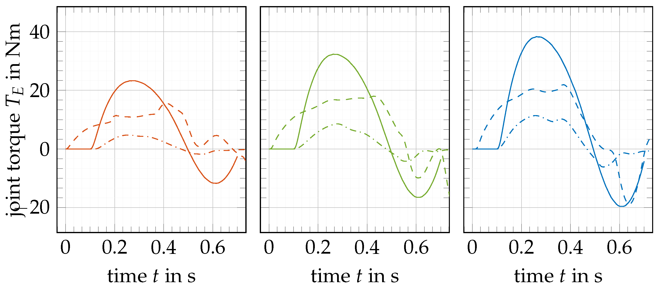
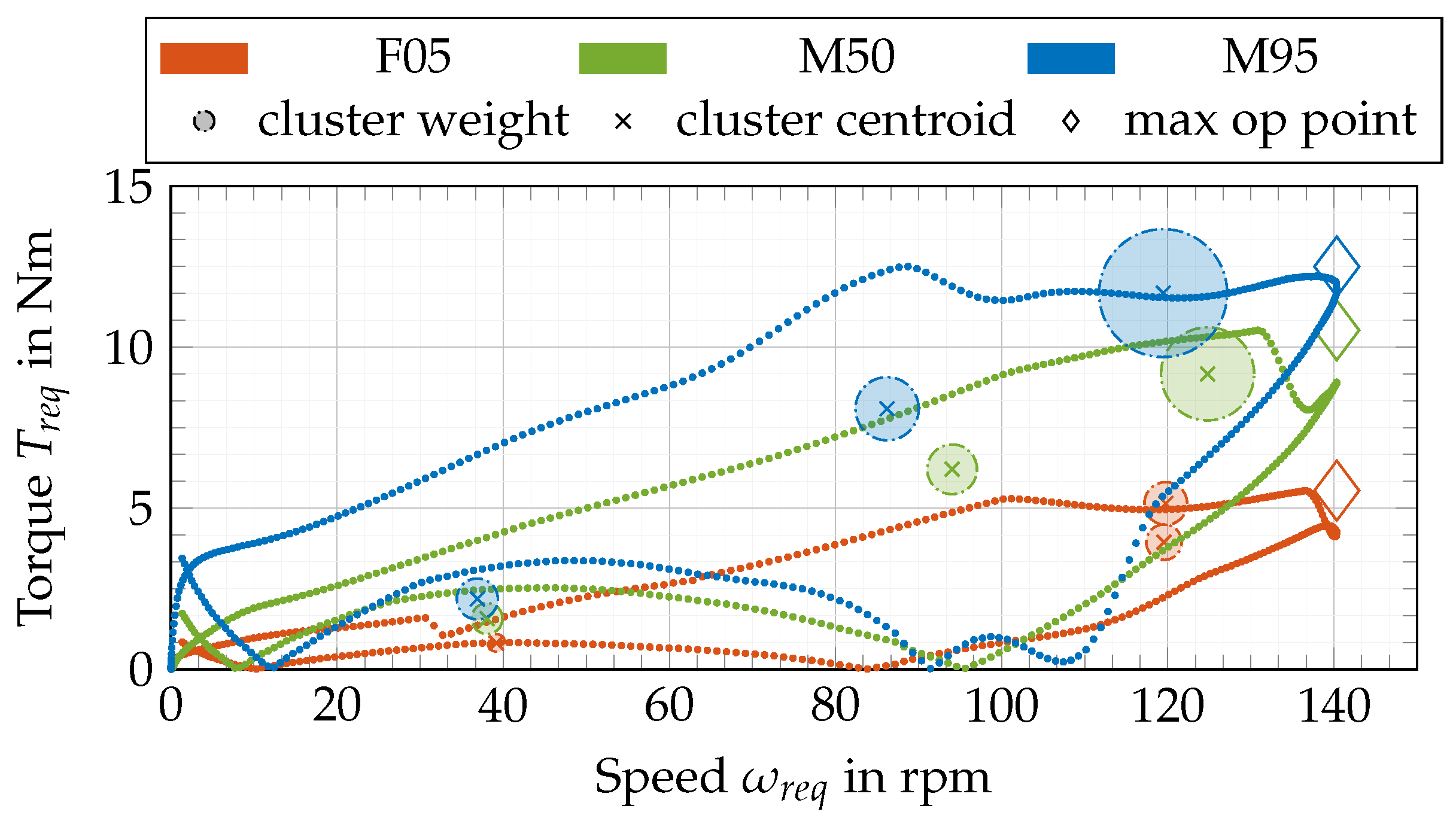
The support torque is individually adjustable. The constant k p e r describes the power factor of the person. If k p e r is set to one, the person will take the full load of the load cycle, which means that there will be no support of the drive unit. If the constant is zero, the weighted movement will feel like the unloaded movement. However, independent of k p e r , the difference in the torque curves is supported to match the optimal trajectory. In Figure 3, exemplary torque curves are visualized. More torque curves are presented in the Appendix A (c.f. Figure A1, Figure A2, Figure A3 and Figure A4). The torque–speed plane was then calculated with (1) and (2) and presented in Figure 4 for three different people for movement A with 100% additional arm weight.
To ensure that all requirements were met, the maximum operating point (maximum speed, maximum torque) was used as the design point for calculating the electric machine. In addition to the maximum operating point, all other operating points are also relevant for the optimum design of the drive, since the loss energy varies in each one, respectively. In this context, partial load points may occur more frequently in a load cycle, where a high efficiency would be desirable. To optimize the overall efficiency over the course of a load cycle, the efficiency has to be considered at each stage thereof. Determining these is very computationally and time consuming for variable electric machines during optimization. Consequently, a reduction of these points needs to be considered. Data downsampling alone could lead to a loss of information about the cycle, which is not recommended. For data reduction, cluster algorithms are a promising approach. Various methods of analyzing driving cycles are presented in the literature [36,37]. Besides the thorough knowledge of experts used to generate relevant operating points, the k-means machine learning algorithm is superior to other algorithms mentioned there. This algorithm generates a centroid by using the Euclidian distance for a given number of clusters under consideration of different similarity constraints [38].
In this approach, in addition to the torque/speed characteristic and considering the physical behavior in the cluster algorithm, the power dissipation was chosen as a supplemental constraint. In robotic applications, especially in this case study, the amount of copper losses is dominant and calculated with
P L , C   =   m k T 2 R p h   T r e p 2 .
Here, the phase resistance R p h , the number of phases m and the torque constant k T of the reference motor were used. Based on the clustering results with three clusters (Figure 4), the elaborated points can be used for electrical machine scaling instead of using all data points. Furthermore, the clusters were weighted based on the time of the cycle within the cluster multiplied by the copper losses related to the total loss power.

2.6. Power Unit Design

2.6.1. Reference Machine

The reference power unit (PU) in this approach consisted of a yokeless double-sided axial flux machine (AFM). In [39], the AFM was geometrically compared to other motor topologies, such as radial and transversal flux machines [40]. The result shows that the AFM is beneficial over other topologies for torque production in flat application fields. The AFM was connected to a harmonic drive gear (HD) by a toothed belt. The optimal gear ratio was designed in accordance with [41], where the stator current of the electrical machine considering a known LC was minimized. This leads to a total gear reduction of i G   =   235 , on average, for different load cycles. The gear ratio is quite high for dynamic applications. This leads to some issues in back drivability of the system, which can be handled through compensating control algorithms. The gear ratio is adaptable and not necessarily fixed for the scaling approach.
Finally, this leads to a design torque of T A F M   =   180 m N m of the AFM. The DC-Link voltage of the reference machine was set to 48 V . Stator housing and coil holders, presented in Figure 5, are made of 3D-printed PLA. Hence, small adjustments in geometry scaling are easily implementable.

2.6.2. Scaling Approach

Figure 6 shows the considered geometry and introduces the geometrical scaling parameters. The general topology was set to a five-phase machine with a stator pole pair number of one. To increase the winding factor, a rotor pole pair number of three was chosen.
The scaling approach utilized in this paper was based on analytical functions that are presented in literature [42,43]. This means varying the machine parameters to a certain extent around the reference machine design. The general scaling law can be given for x as product of x 0 , the considered value of the reference machine and c x , the scaling factor of x. Rearranging this leads to the desired relationship
c x   =   x x 0 .
Further, x can be set to every parameter of the electrical machine and can be defined as x   =   f ( d o u t ,   k D ,   h W ,   ) . Applying (4) to every parameter leads to the general model
c x   =   f ( C d o u t ,   C k D ,   C h W ,   ) .
The general scaling law in (5) can basically be applied to all of the output quantities. For some relationships, it is convenient to introduce so-called auxiliary constants. These will be abbreviated with f x and depend solely on values of the reference machine and physical, material or other auxiliary constants.
In the following, an example for the torque is given. The torque is calculated as
T A F M   =   π 4 ζ w , v   B ^ δ   A A F M d o u t 3 ( k D     k D 3 ) .
The winding factor ζ w , v , the flux density B ^ δ and the current density A A F M are given. In case of the torque equation, the scaling model is defined as
c T   =   T A F M T 0   =   c e l   c m a g n   c g e o m .
For a better understanding of the scaling influences, they can be grouped into electrical, magnetic and geometrical dependencies. In this paper, the geometrical scaling is investigated. Geometrical cross-dependencies to magnetical and electrical scaling are considered. The scaling parameters are defined as λ   =   ( c d o u t ,   c k D ,   c h W ,   c b N ,   c h P M ) T . Further, it is implicated that the electrical and magnetic load of the electrical machine should be constant. In other words, the winding scheme, magnet topology, etc., are fixed. In terms of the magnetic flux density B ^ δ in the air gap, there is a geometric relationship between the height of the permanent magnet h P M and the height of the winding h W . This dependency leads to additional constraints that are considered for the solution of the problem. In (8), (see following page) the torque scaling model is given. Important parts in this equation are the scaling factors for the winding factor c ζ 1 ( λ ) and the edge leakage factor c k L ( λ ) .
The winding factor is investigated in [44]. The scaling behavior was simplified to the carrier wave of the system on the centered radius in this case. Then, the trigonometric functions were mapped to a third grade Taylor polynomial, which maps the function with less than one percent error.
The leakage factor contemplates the edge effects of the permanent magnets on the outer and inner radius of the machine. Furthermore, the shortcut effects between the permanent magnets are taken into account. This factor is based on an average area reduction of the permanent magnet, thus leading to a reduction in the magnetic flux density in the air gap.
In addition, torque c T , speed cw, mass cm, acceleration cα and efficiency cη are defined as necessary values for scaling in personalization for exo drives. The detailed model functions are given in (8) to (12).
The exemplary design area generated from the model (Figure 7) depends on the first three geometric scaling factors of λ . All other scaling factors are kept constant for visualization.
The model provides the opportunity to generate these design areas for all different kinds of scaling factors. To solve the model for the load cycles as defined in Section 2.5, the intersubsection points of these scaling functions must be identified.
c T   =   c N c I c ζ 1 c k L c B r 1   +   f δ f δ 0 c δ + f h P S 0 c h P S + f h W 0 c h W c h P M     1 c d out 2 f K 2   +   1     f K 2 c k D 2
c ω   =   c U i c N c ζ 1 c k L c B r 1   +   f δ f δ 0 c δ + f h S 0 c h P S + f h W 0 c h W c h P M 1 c d out 2 f K 2   +   1     f K 2 c k D 2
c α   =   c T c d out 1 + f Θ 1 c h R   +   c h P M f Θ 2 1     c k D 4 1     1 f K 4
c m   =   c d out 2 1 f m 1   +   f m 2 1     f α 2   +   f F   +   1 c h R f m 1   +   f K 2   +   1     f K 2 c k D 2 c h P M   f m 2 1     f α 2   +   c h P S f F   +   c h W
c η   =   c T   c n f P mech 0 c T c n   +   f P C u 0 c N 2 c l 2 c k C u   c h W   c b N f P C u 1     f P C u 2   c k D c d o u t     f P C u 3   c b N

2.6.3. Solving

The model equations are solved with the Levenberg–Marquardt algorithm, which is based on the least-square algorithm method. The solvability strongly depends on the initial points. Therefore, a multi-start algorithm is used to check a wide range of initial points. A pre-calculated geometrically feasibility check of the initial points restricts the solver to start only with feasible initial points. The solution is based on the following equations. From the load cycle analysis, in combination with the individual body requirements of the user, minimal needed values are identifiable. Therefore, the maximum needed torque T m a x , r e q (see (13)) and the minimum necessary acceleration α m i n , r e q (see (15)) that fulfil the load cycle are determined. Depending on the user, a maximum weight m m a x , u s e r of the electrical machine is chosen (see (14)).
c T ( λ )     T req / T 0   =   0
c m ( λ )     m m a x , u s e r / m 0     0
α m i n , r e q / α 0     c α ( λ )     0
Only in the case of the demanded torque is a strict maximum bond given. For the acceleration and mass, soft maximum and minimum bonds are given. In other words, only the necessary torque should be exactly achieved. Should it be possible through scaling to achieve a lighter motor than the permissible weight or more dynamics as the demanded acceleration for a higher efficiency, the solver can choose this solution. This leads to a better performance of the solver.

2.6.4. Constraints

An important part of scaling definitions is to define the feasible possibilities of the model. Therefore, the following constraints are examined.
For the geometric feasibility, the maximum possible assembly space for the power unit is considered, as well as the space constraint at the inner radius of the AFM. Here, the width of the winding slot has to be small enough to fit two times within the pole pitch of the AFM:
c b N c d o u t   c k D     d o u t   k D 2   b N π m f 1   <   0 .
Under consideration of a parallel slot opening over the machine diameter, the factor f 1 has to be adapted to
f 1   =   sin ( π / m ) .
As mentioned in [39], the double-sided AFM is beneficial over a radial flux machine (RFM) if the assembly space factor c A R is smaller than one. Therefore,
c x 2   f A R 1     c x   f A R 2   +   f x 2 c x 3   c k D f K 2     f K 2     1 c k D 2     1 f A R 0   <   0 ,
is defined, where cx describes the ratio between the outer diameter and the active length in terms of the machine geometry.
Besides the geometric constraints, thermal constraints were implemented as well. The thermal behavior of the AFM was controlled through the maximum allowed current line density. In air-cooled electrical machines, a current line density of 5 10   A / m m 2 is recommended. For short time operations, a current line density of J m a x   =   30 A / m m 2 is permissible [45]. The following constraint is given to
c N   c I c k C u   c b N   c h W     max J 0   <   0 .
Figure 8 shows a design map for an exemplarily designed load cycle (case A) of M50 person. The blue surface shows all scaling combinations that match the torque requirement. Some of the above-mentioned constraints and model equations are displayed as intersubsection lines of the constraint surfaces on the constant torque surface. A further design criterion is the efficiency of the scaled machine. The scaling influence on the efficiency is shown as a contour plot on the constant torque plane. In this case, the efficiency is rising equally to the slot height c h w . Based on these findings, the most efficient scaled machine on the intersubsection lines of (14) and (16) of the possible variants was chosen (see blue dot).

2.6.5. Validation

The model validation is accomplished in two steps: At first, the influences of the scaling parameters are proven by a three-dimensional FEA simulation. Secondly, the reference power unit is built up as a first prototype (see Figure 5) to validate the FEA simulation as well as the analytical model. The measurements are performed on a motor test bench where constant operating points, as well as the earlier mentioned reference load cycle, are implementable. For the speed characteristic, the induced voltage in open circuit operation mode is validated, which indicates the right electromagnetic behavior. For torque and performance validation, the motor is controlled as presented in [46]. Detailed results are given in Table 3 and can be observed as matching very well.
The differences between prototype and FEA simulation are in all values under 1.5%. The maximum deviation between analytical model and prototype is 3.2%, which is acceptable under the assumptions at hand.

3. Results

For the discussion of the results, an exemplary load cycle consisting of the movements “ABCD” and “EFGH” was investigated. Further, the slow load cycle will be called “slc”, and the fast one “flc”.

3.1. Influences of Movement

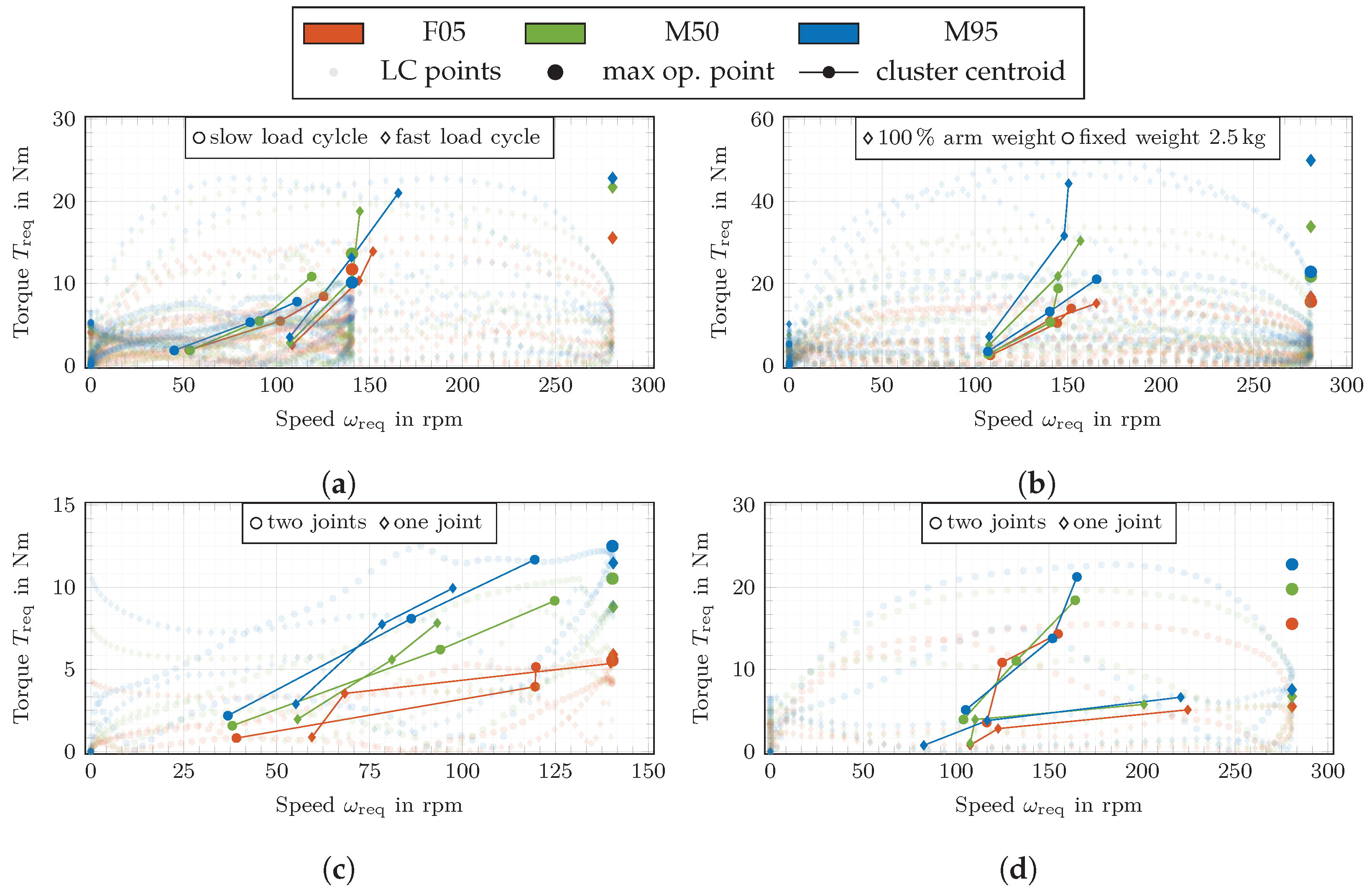
The movement velocity has the largest impact on the load cycle and the requirements of the power unit, as shown in Figure 9a. With a decrease in the movement time, dynamic effects are dominating and the torque necessary to compensate the inertia is rising. In the case of the M95 person, the needed torque rises from 10.11   N m to 22.81   N m . This corresponds to an increase of 125.6%. Furthermore, the power unit speed scales up linearly to the movement velocity. This means that two completely different design points are necessary for the PU designs. Figure 9b shows the difference in the load cycle for different weights. It should be noted that the course of the load cycle remains similar whereas the maximum needed torque scales up linearly. To check the type of movement in Figure 9c,d, movements with different degrees of freedom are shown. In Figure 9c, it is notable that the design point is nearly independent of the movement. On the other hand, the course of the load cycles is different. The cluster points of the single joint movement are shifted into a low speed range, which changes the load cycle efficiency, so the electrical machine has to be adapted. In Figure 9d, the same movements are visualized, only with a shorter duration. In the case of the M95 person, the difference in the demanded torque is between 108% in the slow movement (s. Figure 9c) and 242% in the fast movement (s. Figure 9d). The cross effect to the movement speed is dominant. Further, the cluster points are shifted into a region with higher torques. It can be confirmed, as known in mechatronic systems, that both the type of movement and the speed of movement should be considered in combination and, more precisely, a task-defined load cycle is necessary.

3.2. Influences of Person

Based on the torque–speed profiles, differences caused by the individual person are also noticeable in Figure 9. Due to the different body dimensions, the same activities require different load forces. The comparison of a fixed weight with the weight adjusted to the body mass does not show any differences for the F05 person, whereas the requirements almost double for the M95 person. Figure 9a shows that the dynamic effects also upscale depending on the body dimensions. As mentioned above, concerning the M95 person, the torque demand increases by 125.6 %, and, in the case of the F05 person, by 50%. Furthermore, the simulation shows that the model of the F05 woman cannot lift heavy loads smoothly due to a reduced maximum force in the muscles. This leads to the conclusion that the personalized body dimension will lead to the optimal consideration of the demanded torques.

3.3. Power Unit Scaling

To quantify the benefit of scaling the power modules to the personal needs of the user objectively, the mass of the power module was used as a benchmark characteristic. The mass of the reference motor was compared to the scaled versions. To consider differences in the efficiency of the modules, an additional accumulator mass was calculated. Here, the difference in loss energy over 1000 performed cycles is referred to as the energy density e   =   180 W h k g ( = ^ 648 W s g ) of a lithium-ion accumulator. The formula is given as
Δ m a d d   =   m s c   +   n c y c E V , c u , s c     E V , c u , r e f e     m r e f .
If this additional mass m a d d is smaller than zero, the scaled machine for the considered load cycle is advantageous.
The mass saving of the scaled machines in comparison to the reference machine is given in Table 4. In the case of the slc performed by the F05 person, a mass of 46.7   g is saved. This leads to a reduction of 29.4% of the AFM mass compared to the reference design. Comparing the load cycle slc to flc for the M95 person, the weight saving is 28.4%. Moreover, it needs to be mentioned that the reference power unit could not meet all torque demands. This would lead to a new reference design with additional weight in the case of a standardized solution, which, in turn, leads to more weight saving in other cases. This indicates that the introduced scaling approach is highly beneficial.

4. Discussion and Conclusions

In this paper, a methodology for the individual design of exoskeleton drive units for user- and task-dependent applications was presented. This approach merged a scalable biomechanical human model and a scalable electromagnetic and mechanical model of an electrical machine.
With the scalable human model, forces from arbitrary tasks with different loads are predictable. Thereby, necessary forces for the drive unit design were generated. Alternatively, these forces could be generated from experimental data using an inverse dynamics method, which avoids the model assumptions and limitations presented in [21]. A clear advantage of our method compared to this is that we can easily scale an exoskeleton for different participants based only on the height and weight of the participant. Therefore, we can avoid time-expansive and costly lab measurements.
The analysis of the simulated load cycles shows clear dependencies of the performed task. Among other parameters, the movement speed has a strong influence on the load cycle. In addition, a clear difference is apparent by scaling the human model. Here, in the case of the same movement and load, the force difference between the 5th percentile woman and the 95th percentile man was simulated to 46% related to F05.
Based on these generated forces, a reference elbow power unit was adapted by using the electrical machine scaling model, introduced here in order to meet the exact requirements of the user. The model varies geometrical parameters of the electrical machine to fit the requirements in torque, mass and acceleration. Commercially available motors are not suitable in terms of construction space and power class. Ill-fitting motors cause an oversizing of the power unit, which will lead to additional weight. The typical power density in exoskeleton electrical machines is at 200–300 W / k g . An off-the-shelf motor that meets the performance characteristics introduced here is given a motor weight of 850 g [47]. This is more than five times the weight of the presented reference motor in this journal. Further, the construction space fits in the outer diameter but the axial length of the commercial motor is three times higher, which does not fit in the construction space. Off-the-shelf motors are often limited in scaling and only configurable via a modular system, which is realized by adjusting the active length or the number of windings. The double-sided axial flux machine introduced here, in combination with the additive manufacturing, is easily adaptable to the individual user needs. This scaling leads to a smaller motor weight that saves up to 30% compared to the reference motor. In summary, it can be stated that the scaling presented here enables a significant improvement for the personalization of the electrical machine.
The biomechanical and analytical motor model were validated through experimental data, separately. The measurements used for the biomechanical model are presented in previous investigations [21]. The analytical motor model was validated by a prototype and measurements in this journal. The deviation between the calculation and measurements is below 3.2%, which shows a good suitability of the model. Combined experiments are planned in future research. For a collaborative validation of the approach, a comprehensive ergonomics study with several people wearing a reference exoskeleton on the one hand and a personalized exoskeleton on the other hand is necessary. In this way, objective results on the suitability of the approach can be obtained. These experiments can be realized in future projects.
In addition, the convergence of the biomechanical simulation was used to show which loads can be performed by specific groups of people. Here, it could be observed that the F05 person could not handle as large loads as the M50 or M95 person. This is due to the restricted muscle forces in the model. Thus, in future research, it would be interesting to create a closed coupling between a human and electromechanical model in order to handle heavier loads. Further, human movements can reach speeds of up to 0.2 s for am elbow flexion of 90 degrees. The simulation shows that the actual power unit is not able to support those movement speeds. In ongoing research, the power unit is optimized for such scenarios.
In summary, it is evident that the drive design is improved by the framework presented here and that a lighter design of the exo power unit is possible under consideration of the individual needs of the user and demands of the task.

Supplementary Materials

The following supporting information can be downloaded at: https://www.mdpi.com/article/10.3390/robotics11050107/s1.

Author Contributions

Methodology, software and validation, M.W., I.W., K.S.; supervision and discussion, M.W., I.W., K.S., N.P. and S.S. All authors have read and agreed to the published version of the manuscript.

Funding

The research leading to this publication has received funding from the High-Performance Center Mass Personalization in Stuttgart (https://www.masspersonalization.de/, accessed on 24 August 2022), which was supported by the Ministry of Science, Research and the Arts BadenWürttemberg [Az: 32-7542.2-500/55/3]. Further I. Wochner and S. Schmitt were funded by Deutsche Forschungsgemeinschaft (DFG, German Research Foundation) under Germany’s Excellence Strategy—EXC 2075—390740016. We acknowledge the support by the Stuttgart Center for Simulation Science (SimTech).

Conflicts of Interest

The authors declare no conflict of interest.

Abbreviations

The following abbreviations are used in this manuscript:
AFMAxial Flux Machine
EMElectrical Machine
EMGMuscle Surface Electromyogram
exoExoskeleton
FEMFinite Element Method
HDHarmonic Drive Gear
LCLoad Cycle
PCSAPhysiological Cross-sectional Area
PUPower Unit
RFMRadial Flux Machine

Appendix A. Flexion Movement Load Cycles
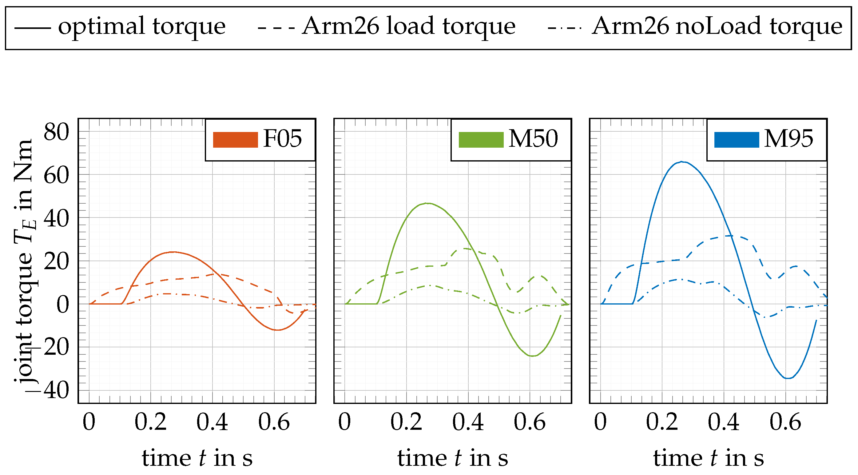
Figure A1. Load profiles for all 3 individuals for m   =   100 % arm weight and case E.
Robotics 11 00107 g0a1
Figure A2. Load profiles for all 3 individuals for m   =   2.5 kg and case E.
Robotics 11 00107 g0a2
Figure A3. Load profiles for all 3 individuals for m   =   100 % arm weight and case A.
Robotics 11 00107 g0a3
Figure A4. Load profiles for all 3 individuals for m   =   2.5 kg and case A.
Robotics 11 00107 g0a4

References

  1. Sylla, N.; Bonnet, V.; Colledani, F.; Fraisse, P. Ergonomic contribution of ABLE exoskeleton in automotive industry. Int. J. Ind. Ergon. 2014, 44, 475–481. [Google Scholar] [CrossRef]
  2. van Engelhoven, L.; Poon, N.; Kazerooni, H.; Barr, A.; Rempel, D.; Harris-Adamson, C. Evaluation of an adjustable support shoulder exoskeleton on static and dynamic overhead tasks. Proc. Hum. Factors Ergon. Soc. Annu. Meet. 2018, 62, 804–808. [Google Scholar] [CrossRef] [Green Version]
  3. Smets, M. A Field Evaluation of Arm-Support Exoskeletons for Overhead Work Applications in Automotive Assembly. IISE Trans. Occup. Ergon. Hum. Factors 2019, 7, 192–198. [Google Scholar] [CrossRef]
  4. Gull, M.A.; Bai, S.; Bak, T. A review on design of upper limb exoskeletons. Robotics 2020, 9, 16. [Google Scholar] [CrossRef] [Green Version]
  5. Shao, Z.F.; Tang, X.; Yi, W. Optimal design of a 3-DOF cable-driven upper arm exoskeleton. Adv. Mech. Eng. 2014, 6, 157096. [Google Scholar] [CrossRef]
  6. Zhou, L.; Li, Y.; Bai, S. A human-centered design optimization approach for robotic exoskeletons through biomechanical simulation. Robot. Auton. Syst. 2017, 91, 337–347. [Google Scholar] [CrossRef]
  7. Zoss, A.; Kazerooni, H. Design of an electrically actuated lower extremity exoskeleton. Adv. Robot. 2006, 20, 967–988. [Google Scholar] [CrossRef] [Green Version]
  8. Toxiri, S.; Calanca, A.; Poliero, T.; Caldwell, D.G.; Ortiz, J. Actuation Requirements for Assistive Exoskeletons: Exploiting Knowledge of Task Dynamics. In Wearable Robotics: Challenges and Trends; Biosystems & Biorobotics; Carrozza, M.C., Micera, S., Pons, J.L., Eds.; Springer: Cham, Switzerland, 2019; Volume 22, pp. 381–385. [Google Scholar] [CrossRef]
  9. Calanca, A.; Toxiri, S.; Costanzi, D.; Sartori, E.; Vicario, R.; Poliero, T.; Di Natali, C.; Caldwell, D.G.; Fiorini, P.; Ortiz, J. Actuation Selection for Assistive Exoskeletons: Matching Capabilities to Task Requirements. IEEE Trans. Neural Syst. Rehabil. Eng. A Publ. IEEE Eng. Med. Biol. Soc. 2020, 28, 2053–2062. [Google Scholar] [CrossRef]
  10. Pries, J.; Hofmann, H. Magnetic and thermal scaling of electric machines. Int. J. Veh. Des. 2013, 61, 219. [Google Scholar] [CrossRef]
  11. Hsieh, K.T.; Kim, B.K. One kind of scaling relations on electromechanical systems. IEEE Trans. Magn. 1997, 33, 240–244. [Google Scholar] [CrossRef]
  12. Zhou, K.; Ivanco, A.; Filipi, Z.; Hofmann, H. Finite-Element-Based Computationally Efficient Scalable Electric Machine Model Suitable for Electrified Powertrain Simulation and Optimization. IEEE Trans. Ind. Appl. 2015, 51, 4435–4445. [Google Scholar] [CrossRef]
  13. Stipetic, S.; Zarko, D.; Popescu, M. Scaling laws for synchronous permanent magnet machines. In Proceedings of the 2015 Tenth International Conference on Ecological Vehicles and Renewable Energies (EVER), Monte Carlo, Monaco, 31 March–2 April 2015; IEEE: Piscataway, NJ, USA, 2015; pp. 1–7. [Google Scholar] [CrossRef]
  14. Seok, S.; Wang, A.; Otten, D.; Kim, S. Actuator design for high force proprioceptive control in fast legged locomotion. In Proceedings of the 2012 IEEE/RSJ International Conference on Intelligent Robots and Systems, Vilamoura-Algarve, Portugal, 7–12 October 2012; IEEE: Piscataway, NJ, USA, 2012. [Google Scholar] [CrossRef]
  15. Wrobel, R.; Mecrow, B. Additive Manufacturing in Construction of Electrical Machines—A Review. In Proceedings of the 2019 IEEE Workshop on Electrical Machines Design, Control and Diagnosis (WEMDCD), Athens, Greece, 22–23 April 2019; Volume 1, pp. 15–22. [Google Scholar] [CrossRef] [Green Version]
  16. Tiismus, H.; Kallaste, A.; Vaimann, T.; Rassolkin, A.; Belahcen, A. Technologies for Additive Manufacturing of Electrical Machines. In Proceedings of the 2019 20th International Conference of Young Specialists on Micro/Nanotechnologies and Electron Devices (EDM), Erlagol, Russia, 29 June–3 July 2019; pp. 651–655. [Google Scholar] [CrossRef] [Green Version]
  17. Kallaste, A.; Vaimann, T.; Rassalkin, A. Additive Design Possibilities of Electrical Machines. In Proceedings of the 2018 IEEE 59th International Scientific Conference on Power and Electrical Engineering of Riga Technical University (RTUCON), Riga, Latvia, 12–13 November 2018; pp. 1–5. [Google Scholar] [CrossRef]
  18. Huang, J.; Huo, W.; Xu, W.; Mohammed, S.; Amirat, Y. Control of Upper-Limb Power-Assist Exoskeleton Using a Human-Robot Interface Based on Motion Intention Recognition. IEEE Trans. Autom. Sci. Eng. 2015, 12, 1257–1270. [Google Scholar] [CrossRef]
  19. Yamasaki, H.; Tagami, Y.; Fujisawa, H.; Hoshi, F.; Nagasaki, H. Interaction torque contributes to planar reaching at slow speed. Biomed. Eng. Online 2008, 7, 27. [Google Scholar] [CrossRef] [Green Version]
  20. Wang, C.; Xiao, Y.; Burdet, E.; Gordon, J.; Schweighofer, N. The duration of reaching movement is longer than predicted by minimum variance. J. Neurophysiol. 2016, 116, 2342–2345. [Google Scholar] [CrossRef]
  21. Stollenmaier, K.; Ilg, W.; Haeufle, D.F.B. Predicting Perturbed Human Arm Movements in a Neuro-Musculoskeletal Model to Investigate the Muscular Force Response. Front. Bioeng. Biotechnol. 2020, 8, 308. [Google Scholar] [CrossRef] [Green Version]
  22. Günther, M.; Schmitt, S.; Wank, V. High-frequency oscillations as a consequence of neglected serial damping in Hill-type muscle models. Biol. Cybern. 2007, 97, 63–79. [Google Scholar] [CrossRef]
  23. Haeufle, D.; Günther, M.; Bayer, A.; Schmitt, S. Hill-type muscle model with serial damping and eccentric force-velocity relation. J. Biomech. 2014, 47, 1531–1536. [Google Scholar] [CrossRef]
  24. Hammer, M.; Günther, M.; Haeufle, D.; Schmitt, S. Tailoring anatomical muscle paths: A sheath-like solution for muscle routing in musculoskeletal computer models. Math. Biosci. 2019, 311, 68–81. [Google Scholar] [CrossRef] [PubMed]
  25. Hatze, H. A myocybernetic control model of skeletal muscle. Biol. Cybern. 1977, 25, 103–119. [Google Scholar] [CrossRef]
  26. Pankoke, S.; Siefert, A. Virtual Simulation of Static and Dynamic Seating Comfort in the Development Process of Automobiles and Automotive Seats: Application of Finite-Element-Occupant-Model CASIMIR; SAE International: Warrendale, PA, USA, 2007. [Google Scholar] [CrossRef]
  27. Decker, W.; Koya, B.; Pak, W.; Untaroiu, C.D.; Gayzik, F.S. Evaluation of finite element human body models for use in a standardized protocol for pedestrian safety assessment. Traffic Inj. Prev. 2019, 20, S32–S36. [Google Scholar] [CrossRef]
  28. Pak, W. Development and Validation of Human Body Finite Element Models for Pedestrian Protection. Ph.D. Thesis, Virginia Tech, Blacksburg, VA, USA, 2019. [Google Scholar]
  29. DIN e.V. (publ.) (DIN 33402-2:2005-12, 2005): Ergonomics—Human Body Dimensions, Part 2: Values. 2005. Available online: https://www.beuth.de/en/standard/din-33402-2/84092742 (accessed on 24 August 2022).
  30. Winter, D.A. Biomechanics and Motor Control of Human Movement; John Wiley & Sons: Hoboken, NJ, USA, 2009. [Google Scholar]
  31. Handsfield, G.G.; Meyer, C.H.; Hart, J.M.; Abel, M.F.; Blemker, S.S. Relationships of 35 lower limb muscles to height and body mass quantified using MRI. J. Biomech. 2014, 47, 631–638. [Google Scholar] [CrossRef] [PubMed]
  32. Flash, T.; Hogan, N. The coordination of arm movements: An experimentally confirmed mathematical model. J. Neurosci. 1985, 5, 1688–1703. [Google Scholar] [CrossRef] [PubMed]
  33. Stollenmaier, K.; Rist, I.S.; Izzi, F.; Haeufle, D.F. Simulating the response of a neuro-musculoskeletal model to assistive forces: Implications for the design of wearables compensating for motor control deficits. In Proceedings of the 2020 8th IEEE RAS/EMBS International Conference for Biomedical Robotics and Biomechatronics (BioRob), New York, NY, USA, 29 November–1 December 2020; IEEE: Piscataway, NJ, USA, 2020; pp. 779–784. [Google Scholar]
  34. Wierzbicka, M.M.; Wiegner, A.W.; Shahani, B.T. Role of agonist and antagonist muscles in fast arm movements in man. Exp. Brain Res. 1986, 63, 331–340. [Google Scholar] [CrossRef] [PubMed]
  35. Kistemaker, D.A.; Van Soest, A.K.J.; Bobbert, M.F. Is equilibrium point control feasible for fast goal-directed single-joint movements? J. Neurophysiol. 2006, 95, 2898–2912. [Google Scholar] [CrossRef]
  36. Gunther, S.; Ulbrich, S.; Hofmann, W. Driving cycle-based design optimization of interior permanent magnet synchronous motor drives for electric vehicle application. In Proceedings of the International Symposium on Power Electronics, Electrical Drives, Automation and Motion (SPEEDAM), Ischia, Italy, 18–20 June 2014; IEEE: Piscataway, NJ, USA, 2014; pp. 25–30. [Google Scholar] [CrossRef]
  37. Salameh, M.; Brown, I.P.; Krishnamurthy, M. Fundamental Evaluation of Data Clustering Approaches for Driving Cycle-Based Machine Design Optimization. IEEE Trans. Transp. Electrif. 2019, 5, 1395–1405. [Google Scholar] [CrossRef]
  38. Selim, S.Z.; Ismail, M.A. K-means-type algorithms: A generalized convergence theorem and characterization of local optimality. IEEE Trans. Pattern Anal. Mach. Intell. 1984, 6, 81–87. [Google Scholar] [CrossRef]
  39. Waldhof, M.; Echle, A.; Parspour, N. A Novel Drive Train Concept for Personalized Upper Body Exoskeletons with a Multiphase Axial Flux Machine. In Proceedings of the 2019 IEEE International Electric Machines & Drives Conference (IEMDC), San Diego, CA, USA, 12–15 May 2019; IEEE: Piscataway, NJ, USA, 2019; pp. 2160–2166. [Google Scholar] [CrossRef]
  40. Keller, M.; Müller, S.; Parspour, N. Design of a transverse flux machine as joint drive for an articulated six-axis robot arm. In Proceedings of the 2016 International Symposium on Power Electronics, Electrical Drives, Automation and Motion (SPEEDAM), Capri, Italy, 22–24 June 2016; pp. 849–854. [Google Scholar] [CrossRef]
  41. Bartlett, H.L.; Lawson, B.E.; Goldfarb, M. Optimal Transmission Ratio Selection for Electric Motor Driven Actuators With Known Output Torque and Motion Trajectories. J. Dyn. Syst. Meas. Control 2017, 139, 43. [Google Scholar] [CrossRef] [Green Version]
  42. Hanselman, D.C. Brushless Permanent-Magnet Motor Design; McGraw-Hill: New York, NY, USA, 1994. [Google Scholar]
  43. Gieras, J.F.; Wang, R.J.; Kamper, M.J. Axial Flux Permanent Magnet Brushless Machines, 2nd ed.; Springer: New York, NY, USA, 2008. [Google Scholar]
  44. Kamper, M.J.; Wang, R.J.; Rossouw, F.G. Analysis and Performance of Axial Flux Permanent-Magnet Machine with Air-Cored Nonoverlapping Concentrated Stator Windings. IEEE Trans. Ind. Appl. 2008, 44, 1495–1504. [Google Scholar] [CrossRef]
  45. Rosu, M.; Zhou, P.; Lin, D.; Ionel, D.M.; Popescu, M.; Blaabjerg, F.; Rallabandi, V.; Staton, D. Multiphysics Simulation by Design for Electrical Machines, Power Electronics and Drives; IEEE Press Series on Power Engineering; Wiley: Hoboken, NJ, USA, 2018; Volume 66. [Google Scholar]
  46. Waldhof, M.; Parspour, N. Torque Ripple Minimization in Exoskeleton Drives with Multiphase Electrical Machines by Current Harmonic Injection. In Proceedings of the 2020 International Conference on Electrical Machines (ICEM), Gothenburg, Sweden, 23–26 August 2020; Volume 1, pp. 2152–2158. [Google Scholar] [CrossRef]
  47. Maxon-Motor-GmbH. Available online: https://www.maxongroup.de/maxon/view/category/motor?etcc_cu=onsite&etcc_med_onsite=Product&etcc_cmp_onsite=ECXSPEEDProgramm&etcc_plc=Overview-Page-brushless-DC-Motors&etcc_var=[de]#de#_d_&target=filter&filterCategory=ECX (accessed on 21 March 2022).
Figure 1. Schematic overview of the design method in this approach.
Robotics 11 00107 g001
Figure 2. Visualization of arm model with the considered movement matrix. In (a), the defined angles are shown. (b,c) show the start and target positions of the movements as well as the controlled trajectory.
Robotics 11 00107 g002
Figure 3. Simulated load cycle comparison for the movements, case A and E (see Table 1), with different movement durations t m o v and loads m l o a d . The solid black line shows the optimal trajectory and torque curve T l o a d , o p t of the M50 with 100% arm weight. In (a,b) the joint angles of the elbow and in (c,d) the resulting torque in the elbow joint during the performed task are presented. Further, in (c), exemplary for M50, the torque curves used in (1) are marked.
Robotics 11 00107 g003
Figure 4. Clustering result for all persons for case A with the relative weight of 100% arm weight and a support of k p e r   =   0.5 . The cluster centroids with their statistical weight. The size of the cluster weight circle shows how many points and how much loss power are grouped in this cluster, statistically related to the number of all points and total loss power of the load cycle. The maximum operation point later is used as EM design point.
Robotics 11 00107 g004
Figure 5. Reference power unit design prototype. (a) Power unit for an elbow. All housing components are made of 3D-printed PLA. (b) 3D-printed coil holders with winding.
Robotics 11 00107 g005
Figure 6. Geometry drawings of yokeless double-sided axial flux machine with relevant design parameters. The outer diameter of the AFM is expressed by d o u t . The ratio between the inner diameter and the outer diameter is expressed through k D . The winding area is defined through the height h W and the width b N . The coil width is defined with τ C . The winding is implemented parallel along radial direction. The heights of the permanent magnets h P M and the width τ p m are shown. The rotor height is given with h R . (a) Cut view on the middle radius. (b) Top view.
Robotics 11 00107 g006
Figure 7. Model dependency on three exemplary different scale factors. The iso-surfaces visualize the scaling of the torque. The contour lines in the axes limit show the scaling for all model outputs.
Robotics 11 00107 g007
Figure 8. Solution map for the elbow power unit of a M50 at the movement case A.
Robotics 11 00107 g008
Figure 9. Comparison of load cycle data based on several criteria. Besides the load cycle data points (low opacity in background), the cluster centroids of the k-means algorithm are displayed. The cluster weight is not further visualized. As electrical machine design point, the maximum operation point is used. (a) Load profiles slc and flc with a fixed weight of 2.5 kg. (b) flc with fixed load at 2.5 kg and referred load at 100% arm weight. (c) Movements of case A vs. C with an additional load of 100% arm weight. (d) Movements of case E vs. G with an additional fixed weight of 2.5 kg.
Robotics 11 00107 g009
Table 1. Movement matrix.
CasesStart to Target Angle [ Θ E , Θ S ]Mov. DurationDoF
A[00 ,00 ]to[−90 ,−90 ]flex. 1.2   s two joints
B[−90 ,−90 ]to[00 ,00 ]ext. 1.2   s two joints
C[00 ,00 ]to[00 ,−90 ]flex. 1.2   s one joint
D[00 ,−90 ]to[00 ,00 ]ext. 1.2   s one joint
E[00 ,00 ]to[−90 ,−90 ]flex. 0.6   s two joints
F[−90 ,−90 ]to[00 ,00 ]ext. 0.6   s two joints
G[00 ,00 ]to[00 ,−90 ]flex. 0.6   s one joint
H[00 ,−90 ]to[00 ,00 ]ext. 0.6   s one joint
Table 2. Total height and weight for three typical human percentiles commonly used in ergonomic studies.
DescriptionUnitF05M50M95
total height lB  m 1.5351.7501.855
total weight mB  kg 52.00079.000100.000
Table 3. Result comparison from the analytical model (AM), 3D finite element analysis (FEA) and measurements of the prototype (PT).
ParameterUnitAMFEAPT
Torque TAFM m N m 180.80178.90176.20
Ind. Voltage UimV/rpm1.541.491.49
Mass m r e q g 156.15156.35157.20
Efficiency η 1%62.4962.2561.90
1 at n = 3000 rpm, i ^ 1   =   5 A .
Table 4. Weight differences between the reference machine and scaled electrical machines for exemplary load cycles with different load weights and a total number of cycles n c y c = 1000 .
Load CyclePerson m l o a d  [g] η L C  [%] Δ m a d d  [g]
slcF052.533.8−46.7
M502.543.8−44.3
M952.537.9−39.6
F052.630.9−40.5
M503.9549.2−25.7
M95557.6−9.7
flcF052.551.3−32.2
M502.567.2−15.8
M952.574.26.8
F052.652.4−28.7
M50 1 3.9573.414.5
M95 1 577.842.63
1 Reference machine does not fulfil all maximum requirements.
Publisher’s Note: MDPI stays neutral with regard to jurisdictional claims in published maps and institutional affiliations.