Abstract
This paper presents a method of optimizing the design of robotic manipulators using a novel kinematic model pruning technique. The optimization departs from an predefined candidate linkage consisting of a initial topology and geometry. It allows simultaneously optimizing the degree of freedom, the link lengths and other kinematic or dynamic performance criteria, while enabling the manipulator to follow the desired end-effector position and avoid collisions with the environment or itself. Current methods for design optimization rely on dedicated and complex frameworks, and solve the design optimization only as decoupled from each other in separate optimization problems. The proposed method only requires the introduction of a simple function, called a pruning function, as an objective function of an optimization problem. The introduced pruning function transforms a discrete topology optimization problem into a continuous problem that then can be solved simultaneously with other continuous objectives, using readily available optimization schemes. Two applications are presented: the optimization of a manipulator for the inspection of radio frequency cavities and a manipulator for maintenance within the future circular collider (FCC).
1. Introduction
Power plants and big industrial or scientific facilities like the European Organization for Nuclear Research (CERN), are often confronted with very special automation problems in complex environments for their laboratories, experiments or test rigs, see e.g., [1,2]. These frequently lead to specific requirements that do not allow the usage of standard industrial robots. Thus, a robotic design problem with few restrictions on the actual robot design (topology and geometry), but with very hard requirements concerning other parameters, such as workspace, allowed robot space, dexterity and accuracy, has to be solved.
Design optimization in robotics is a recurrent topic and has been discussed in the literature from many different perspectives. Several publications address the continuous optimization problem of minimizing certain deterministic (mainly kinematic or dynamic) performance criteria for a given topology, as shown in [3,4,5,6,7]. All of the above mentioned articles use different performance criteria, optimization techniques and solvers or approaches for collision avoidance, but non of them minimize the degrees of freedom (DoF) of the mechanical structure. The discrete problem of minimizing the DoF/topology is solved, in the literature, by always decoupling it from the previously mentioned continuous optimization tasks. Extensive frameworks for structural synthesis are presented in [8,9], which start by exploring all possible combinations of joints and links. Then, the these topologies can be optimized with respect to deterministic performance criteria. Ref. [10] proposes a smart framework to optimize the link lengths and other performance criteria, but mentions that discrete criteria, such as the number of actuators, cannot be handled, since the optimization strategy requires the first and second derivatives. Based on these findings [11] extends the framework in order to enable the use of discrete criteria, but the optimization of discrete and continuous criteria are still decoupled into two separate optimization problems. Thus, complete design optimizations, in terms of topology and geometry, currently requires dedicated and complex frameworks that optimize both objectives only as decoupled from each other into two separate optimization problems.
In order to alleviate the complexity problem, in the following, a synthesis approach is presented that allows simultaneously optimizing the link length as well as the DoF. The approach is based on a candidate linkage and a pruning method that is used to optimize the candidate linkages. In other words, this work proposes a kinematic model pruning technique to simultaneously optimize discrete (topology/minimizing the DoF) and continuous criteria (link lengths, kinematic and dynamic performance criteria). The focus of this paper is the formulation of the optimization problem, but not its numerical solution (to this end, standard numerical solvers are applied). To achieve the simultaneous optimization of topology and geometric parameters, a certain type of function (hereafter called the pruning function) that facilitates the transformation from a discrete to a continuous problem, is defined. Thus, the presented kinematic model pruning technique allows optimizing the degrees of freedom, the robot link lengths and other kinematic or dynamic criteria, while ensuring that the mechanical structure reaches the desired end-effector position, avoids self collisions and collisions with its surrounding. This will be demonstrated with two applications:
- The design optimization of a surface inspection robot for radio frequency (RF) cavities, as used in the Large Hardron Collider (LHC), the Linear Accelerator (LINAC) or the Future Circular Collider (FCC).
- The design optimization of a manipulator for the 100-km-long FCC.
Section 2 summarizes the goals and limitations of the design optimization. In Section 3 the methods and work flow of the proposed algorithm are presented, and Section 4 describes the generic formulation of the design optimization algorithm in detail. In Section 5 and Section 6 the proposed technique is applied to two specific problems, the cavity inspection robot and the robotic manipulator for the FCC. The last Section 7 summarizes the results and draws conclusions concerning the existing and future work.
2. Design Optimization Goals and Limitations
The proposed method is capable of modifying an initial and, thus, non-optimal candidate linkage that defines a variety of possible topologies, called design space (see Section 3.1). Simultaneously the geometry of the mechanical structure will be tuned such that the final result provides an optimal and practically feasible solution with respect to certain objectives:
- minimize the DoF;
- minimize the length of each robot link; and
- minimize kinematic and dynamic performance criteria of the mechanical structure.
These objectives should be optimized such that the robot is able to reach all desired positions and avoid collisions with itself as well as with the environment. The algorithm is, in general, applicable under following constraints:
- the topology can consist of arbitrary joint types, but only subsequent joints of the same type can be use for reducing the DoF; and
- the additional kinematic and dynamic performance criteria subject to optimization should, in the best case, be complementary, but never be in contradiction with each other.
3. Methodology
Figure 1 visualizes the workflow of the proposed algorithm and shows how the different methods are connected. The design optimization departs from a predefined design space (see Section 3.1), which will then be exploited by the kinematic model pruning method (see Section 3.2) in order to find the optimal design (see Section 3.3).
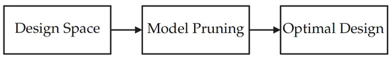
Figure 1.
Workflow of the Design Optimization.
3.1. Design Space
The design space describes a variety of possible topologies based on predefined assumptions by the user. It is defined by a candidate linkage in the form of a topology and geometric parameters, see e.g., Figure 8 and Table 1. The DoF of the predefined design space needs to be greater than the expected optimal solution, since the algorithm is only able to reduce, and not increase, the DoF.
3.2. Kinematic Model Pruning
The kinematic model pruning block in Figure 1 consists of a continuous optimization problem that is to be solved using readily available optimization schemes. For detailed information about the implementation and formulation of the optimization problem see Section 4. However, the focus of this paper is the formulation of the optimization problem, but not its numerical solution (to this end standard numerical solvers are applied). As discussed in Section 1 the challenge is to combine the discrete and continuous criteria in order to be able to formulate only one optimization problem that takes all goals from Section 2 into account. At the core of the proposed kinematic model pruning technique is a certain type of function called pruning function, see Definition 1. Setting this function as the objective function enables the transformation of the discrete topology optimization problem into a continuous problem. Therefore, the topology can be optimized simultaneously with other continuous criteria or goals as presented in Section 2. The pruning function is a simple vector function with two inequality constraints on the first and second derivative.
Definition 1
(pruning function). A vector function with argument that satisfies
and
Constraint (1) ensures that the design parameters will be minimized and constraint (2) drives the design parameters to zero. In other words, constraint (2) facilitates minimization of a discrete problem like the number of DoF in a mechanical structure. In the following Example 1, the behavior of the rather abstract Definition 1 will be demonstrated with the optimization of a simple two-DoF planar robotic manipulator. Furthermore, the results of the optimization with a pruning function will be compared to the results using a quadratic function for the objective function.
Example 1.

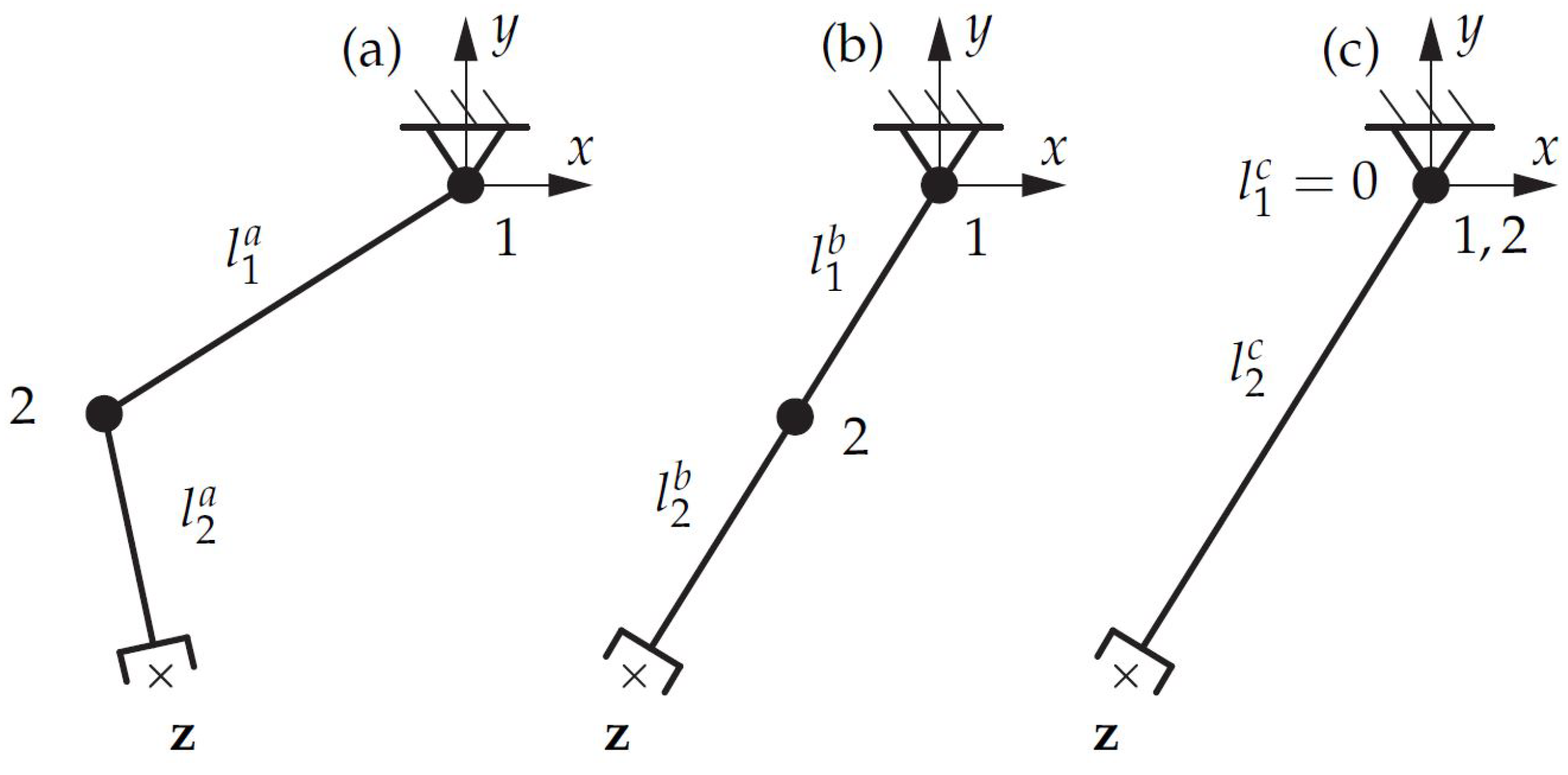
The end effector of an link planar manipulator with two DoF should be able to reach exactly one point at position . Note that the orientation will not be constrained, thus creating a task redundancy. In Figure 2a the initial design, with two DoF and the link lengths and , is shown. Departing from this candidate linkage, the optimization should find an optimal design with minimal link lengths and a minimal number of DoF, while still reaching the desired position . A corresponding optimization problem
with the objective function can be formalized. denotes the forward kinematics, vector contains the two geometric parameters or link lengths, vector contains the two joint angles and vector is used as a weighting factor. For demonstration purposes, the optimization will be launched twice with different functions for . Once with a pruning function (see Definition 1)
and once with a quadratic function ,
with the well-known properties
Figure 2.
Optimization effects using different function types for . (a) shows the design space. (b) shows the optimization results using a quadratic objective function. (c) shows the optimization results using kinematic model pruning.
Note that the second derivative of the quadratic function is, unlike for the pruning function, greater than zero.
The optimization result, when using a quadratic objective function , is shown in Figure 2b. It is obvious that the optimization converges to an optimum, since the links lie on a straight line, in Euclidean space, from the base to the desired end-effector position. However, it is also clear that only one DoF would be sufficient to reach this position. Thus, it is easy to see that the quadratic objective function minimizes the total length , but splits up this length equally over both links, such that and, hence, does not minimize the DoF.
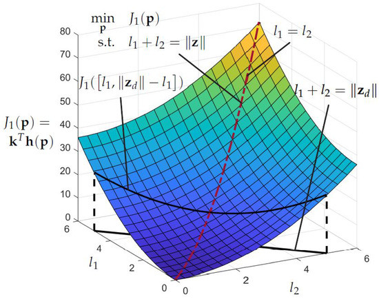
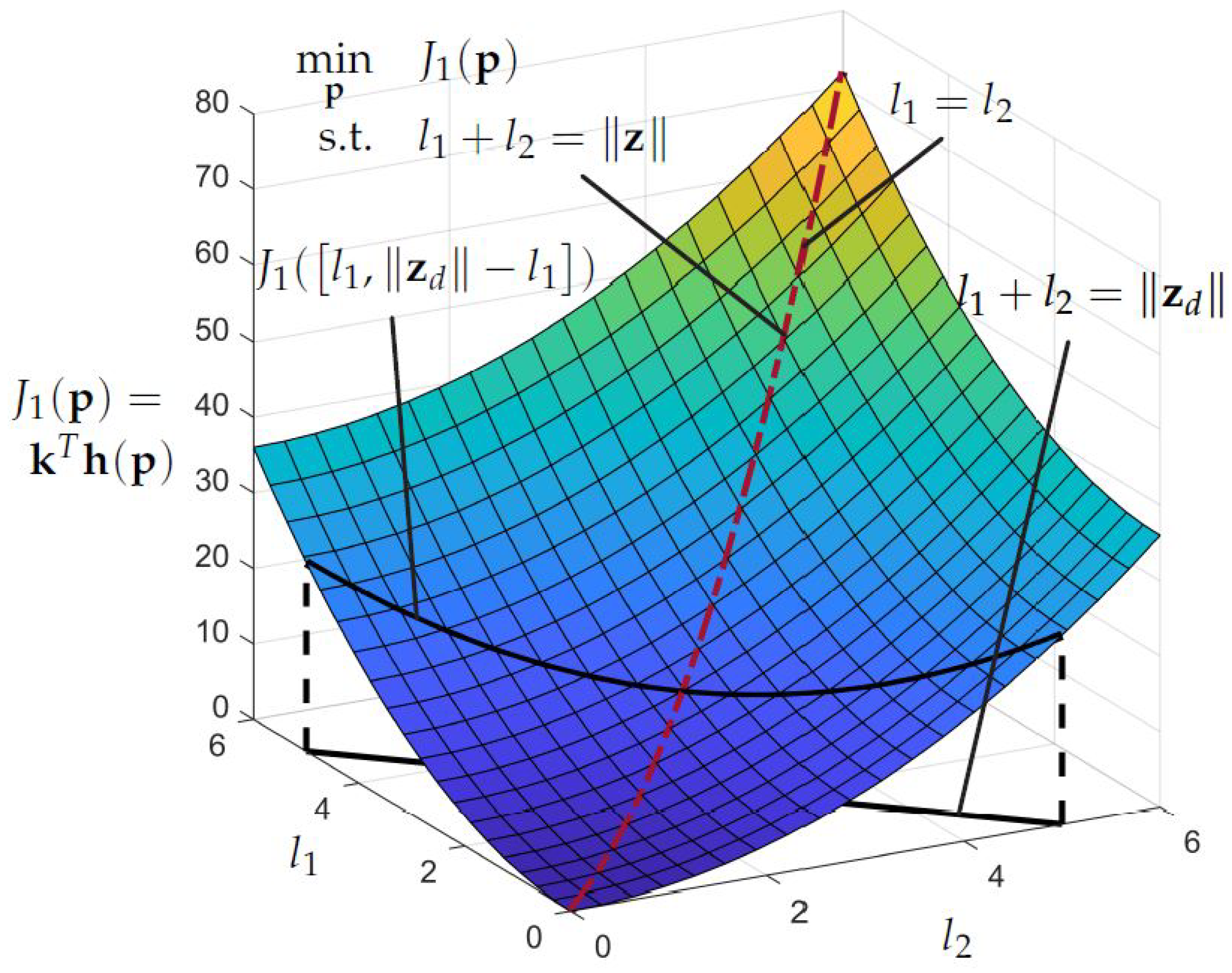
This behavior becomes more clear when looking at the surface and contour plots of the objective function over the variables and as shown in Figure 3 and Figure 4, respectively.
Figure 3.
Surface plot of objective function .
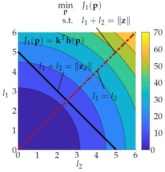
Figure 4.
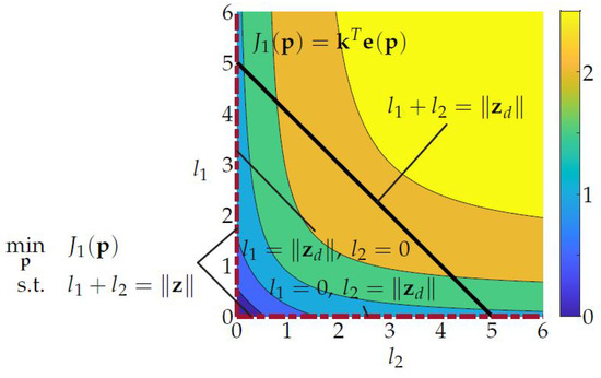
Contour plot of objective function .
The black line in the plane represents the possible combinations of and with which the desired end-effector position can be reached and holds. The projection of this line on the surface of leads to the curved line from which the optimal combination of and has to be chosen. The dashed red line visualizes the space of optimal combinations of and for arbitrary , which is identical to the space of combinations wherein . This becomes even more clear when looking at the contour plot in Figure 4. The black line shows a -45 slope and the contour lines are circles of different diameter centered at the origin. Thus, the optimal solution can be found where the line intersects exactly once with a contour line or in other words, where the line is a tangent to the contour line. For arbitrary , this leads to optimal solution .
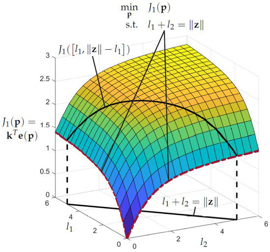
In order to minimize the DoF the distance should not be split up equally, but assigned to only one link, while the other link length will be set to zero. The corresponding joint to this link can then be removed, which means decreasing the DoF by one. This behavior can be achieved by using a pruning function (see Definition 1), specifically (4) for in (3). Running the same optimization problem again with the new objective function, the total link length is still a minimum (straight line in Euclidean space), but is now assigned to only one link. This indicates that not more than one DoF is necessary to reach the position (see Figure 2c). Thus, the corresponding joint i with can be removed and the link lengths, and the DoF is minimized.
Again, this behavior becomes more clear when looking at the surface and contour plots of the objective function over the variables and , as shown in Figure 5 and Figure 6, respectively.
Figure 5.
Surface plot of the objective function .
Figure 6.
Contour plot of objective function .
The black line in the plane represents the possible combinations of and with which the desired end-effector position can be reached, and holds. The projection of this line on the surface of leads to the curved line from which the optimal combination of and has to be chosen. The dashed red lines visualize the space of optimal combinations of and for arbitrary . Compared with Figure 3 it can now be seen that for every two solutions and with the same priority (for the special case ) exist. Both solution lie at the lower boundaries of the parameters and . This becomes even more clear when looking at the contour plot in Figure 6. The black line shows again a −45 slope, but now the contour lines are shaped in way such that the optimal solutions lie at the boundaries of . The optimal solution can be found by restricting the parameters with upper bounds in the optimization problem leading to only one solution e.g., .
3.3. Optimal Design
The optimal design consists of the original topology, as defined in the design space, plus a set of optimal design parameters or geometric parameters. If one of the geometric parameters is driven to zero by the kinematic model pruning method, then this indicates a possible reduction of DoF and the corresponding joint can be removed.
4. Formulation of the Design Optimization Problem
In the following, the implementation and formulation of the optimization problem will be shown in more detail. In this section the problem is described in a generic manner in order to allow an easy extension of the problem with e.g., performance criteria that were not considered in this work. Specific implementations for certain problems are presented in Section 5 and Section 6. In Section 4.1 a parameterized model of the initial mechanical structure, including kinematics and dynamics, are defined. General assumptions on the collision avoidance are discussed in Section 4.2. The formulation of the optimization problem is shown in Section 4.3 and the applied objective function is described in Section 4.4.
4.1. Kinematic and Dynamic Model
The forward kinematics , with degrees of freedom n and in Cartesian positions, can be written in the form
with the Cartesian positions and orientations , the N geometric parameters and the generalized joint coordinates for every Cartesian position written in vector
An explicit solution for the inverse kinematics is not computed, since it will be taken into account by non-linear equality constraints in the optimization problem.
The forward dynamics or the equation of movement for the entire robot can be written as
with the mass matrix , the non-linear term containing gravitational, centrifugal and Coriolis terms and the actuator and external forces and torques .
4.2. Collision Avoidance
To reduce the computational cost of the simulation, it was assumed that the mechanical design either prevents two consecutive links to collide or the collision avoidance is handled by bounds on the corresponding joint angles. Thus, for an serial-link robot
self collisions and, in general,
collisions with the environment have to be monitored.
4.3. Problem Formulation
The optimization was set up as a non-linear global optimization problem with non-linear equality and inequality constraints
with the objective function and the N geometric parameters or link lengths of the candidate linkage
The vector , see (8), contains the generalized coordinates in joint space for different desired Cartesian positions
The inverse kinematics is included with the equality constraint
The vector function
contains the minimal distances according to self-collisions and collisions with the environment. The vector functions
are upper and lower bounds on the joint angles and link lengths.
4.4. Objective Function
As already discussed in Section 2, the desired objective function should minimize the DoF, the robot link lengths and other kinematic and dynamic performance criteria. This is expressed as linear combination of the objectives
In the following Section 4.4.1 and Section 4.4.2 the intended effects of and on the optimization problem are discussed. The term penalizes the length of the robot links with a mapping and the weighting factor . The term represents kinematic and dynamic criteria summarized in , which is weighted with the diagonal matrix .
4.4.1. Minimizing the DoF and Link Lengths
The term penalizes the robot link lengths in a way such that both the link lengths and the DoF of the robot are minimized. This requires a specific type of function, called pruning function (see Definition 1), for in (18). A more detailed demonstration of the behavior of pruning functions is shown in Example 1. As a result, the total link length of the mechanical structure is minimized and, if possible (with respect to all constraints), geometric parameters are driven to zero and, thus, indicate a possible reduction of DoF.
4.4.2. Minimizing Kinematic and Dynamic Performance Criteria
The term of (18) accounts for arbitrary kinematic or dynamic criteria summarized in vector and multiplied with a weighting matrix . It is important that multiple criteria do not contradict each other or, in the best case, are complementary, in order to avoid ill-conditioned optimization problems. Possible criteria are the motor torque, distance from singularities, error propagation through the mechanical structure or kinematic and dynamic manipulabilities. Examples for such criteria are shown in Section 5.3 and Section 6.2.
5. Application: Cavity Inspection Robot
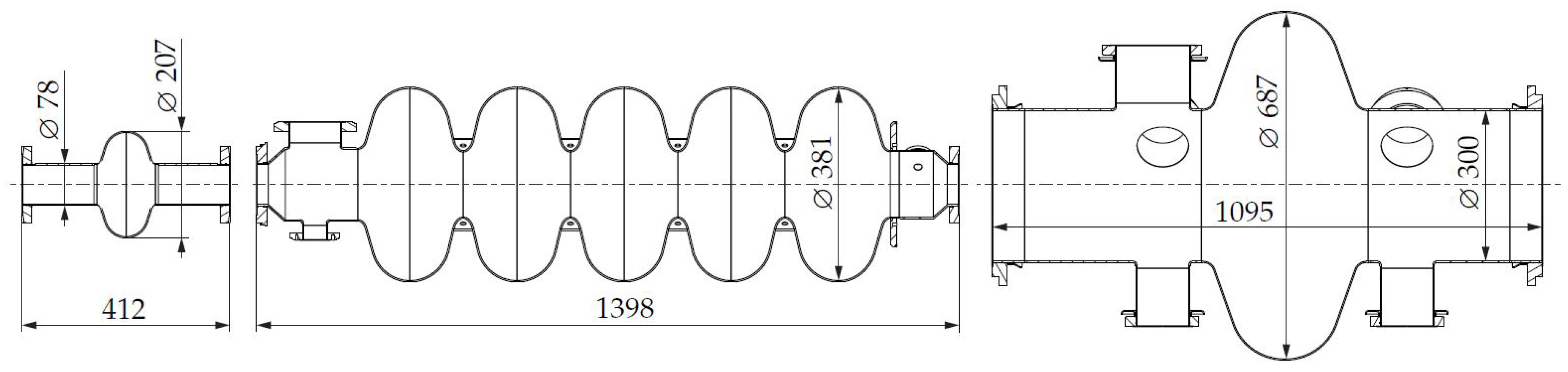
Radio frequency cavities (see Figure 7) perform the linear acceleration of charged particles in straight sections of accelerator machines and, thus, make up one of the key elements in a collider complex [12]. The cavities structure and geometry define their specific radio-frequency at which the strong electromagnetic field, created inside the tubes, oscillates to accelerate each particle passing through. The inner surface quality of the cavities is critical for withstanding high energy densities, since every scratch or crack leads to higher local resistance and, thus, a rapid increase in temperature during operation and, in the end, to the failure of the system. Therefore, some kind of automated, mechanical structure has to follow the complex cavity geometry and take records of the surface quality after full assembly of the cavities. Finding the optimal topology of such a mechanical structure with respect to certain constraints, such as collision avoidance for different cavity types and minimal error propagation in direction perpendicular to the cavity surface, is a perfect example of the generic problem described in Section 1. Currently, several different system have been developed and are able to partially scan cavities (see [13,14,15,16]). However, those previously developed cavity inspection systems were extensively tested at CERN but did not satisfy the specific requirements concerning the level of automation, accuracy, repeatability and how much of the inner cavity surface could be inspected and mapped. The first prototype of the system developed at CERN and presented in [1] was not able to scan all three cavities with one robotic arm, but had to use two different arms. The aim of this design optimization is to find one topology and geometry that can handle all three cavity types and thus increase robustness and level of automation while decreasing the cost of such a system.
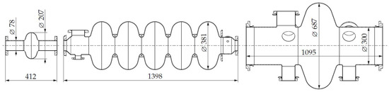
Figure 7.
Cavity types for FCC, LINAC and LHC (left to right, all units in mm).
The main challenge for a robotic system is the complex workspace and, especially, the difference in diameter of the entrance of the smallest cavity (FCC) and the point with maximum diameter of the biggest cavity (LHC). Furthermore, the system has to detect surface anomalies of only m. A 18MP camera with liquid lens, allowing it to focus between 20 to 25 mm, is used. In order to provide one full image of the inner surface, the cavities are rotated around their axes of symmetry, while robotic manipulators are inserted along these axes. The pictures are stitched together after the inspection. Thus, the accuracy error of the end-effector position tangential to cavity surface should be not more than 1.2 mm to obtain only 10% overlapping error and not more than 1mm in the direction perpendicular to the cavity surface, which otherwise changes the contained surface area in the image.
In Section 5.1 the initial model and geometry and the projection equation [17] to derive the equation of motion is described. Section 5.2 illustrates the collision-checking procedure and Section 5.3 presents the applied kinematic criteria for this example. Then, the initial states and results of the optimization are shown in Section 5.4 and Section 5.5, respectively.
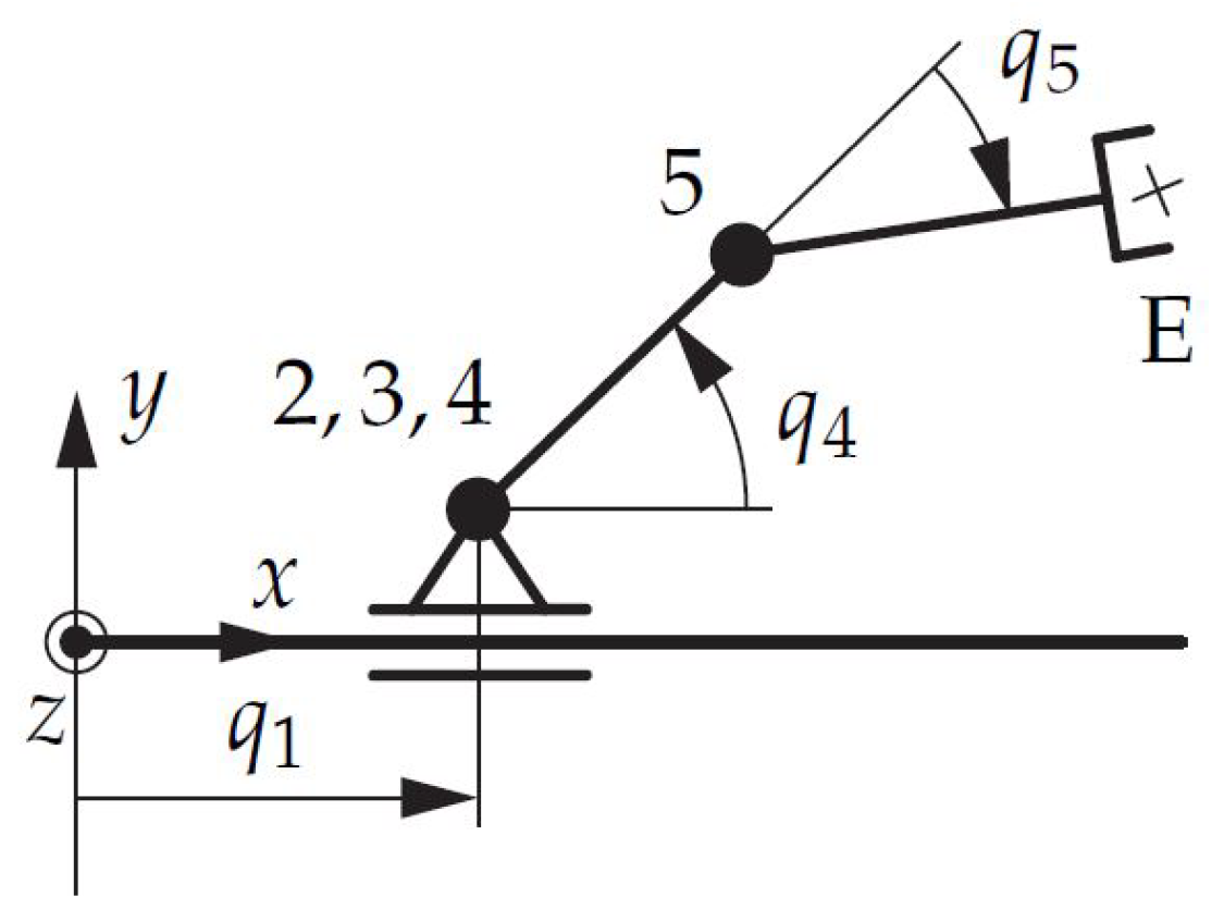
5.1. Model
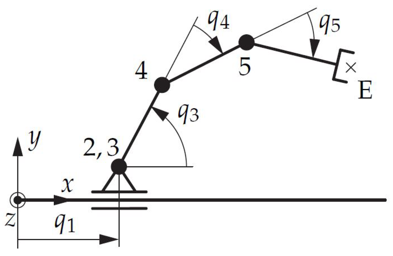
The surrogate model defining the design space has been set up with one translational and four rotational joints with parallel rotation axes, summing up to five DoF, as shown in Figure 8. Table 1 lists the initial link lengths, where describes the lengths from joint i to joint j. These lengths are evaluated by launching an optimization problem, as described in Section 5.4, that returns feasible initial states. This initial set up has been used as the starting point for the actual optimization problem in (12).
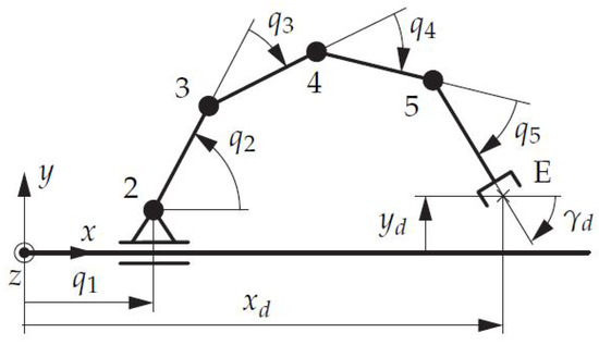
Figure 8.
Design space.

Table 1.
Initial geometry.
The generalized joint coordinates are set to
and the desired Cartesian position and orientation are
with the position and and the orientation around the z-axis always keeping the end-effector orientation perpendicular to the cavity surface. The optimization parameter is set to
with the different cavities and different positions leading to . The parameter vector is defined as
5.2. Collision Avoidance
The collisions between robot and environment are calculated by discretizing the cavity surfaces and checking the minimal distances between robot links and points on the cavity surface. First, all points on the cavity surface are transformed into the body fixed coordinate frames for each robot link and then, to decrease the computation time, only points that can possibly collide and, thus, lie in the selected points area (see Figure 9) are considered. The minimal value of the projection of all possible collision points onto the y axis of the body-fixed coordinate frame is considered the minimal distance. Collisions are taken into account in the function in (12). Self collisions between robot links are not considered, since it is assumed that this is mechanically impossible, as known from Scara robots.
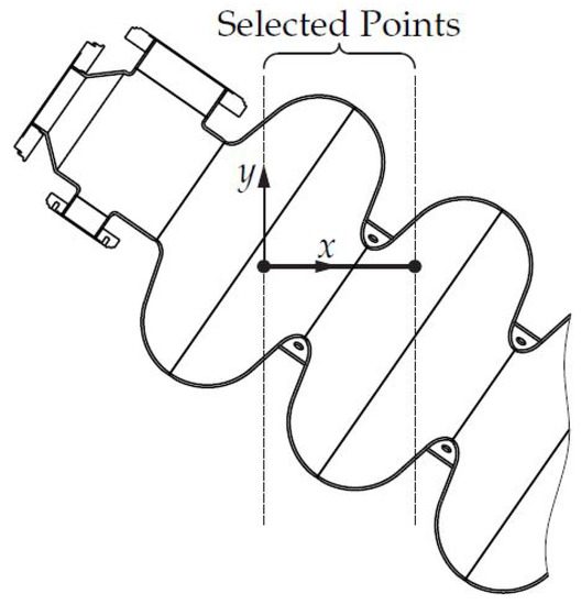
Figure 9.
Collision detection for one robot link.
5.3. Kinematic and Dynamic Performance Criteria
It is crucial for the cavity inspection robot to provide a very stable base for the camera that is being used for the inspection process, since the errors that should be detected in the surface can be only micro fractures. Thus, the term of (18) is set up to optimize the error propagation through the mechanical structure in a certain direction of interest. Error propagation describes how errors that originate in joint space are being forwarded to the end-effector, such as, e.g., gear elasticity, backlash or control oscillations. This can be quantified using the directional kinematic manipulability [18]
with the unit vector representing the direction of interest (perpendicular to the cavity surface) and the major and minor axes of the manipulability ellipsoid obtained from the singular value decomposition of the geometric Jacobian
with the linear and angular end-effector velocities and , respectively. Looking at the mapping from joint to Cartesian space via the Jacobian and replacing the small changes in joint angles with an error , the error in Cartesian space is
Thus, for a robot in a singular configuration such as the two-link arm in Figure 2b, the error propagation in direction of the eigenvector corresponding to the smallest singular value is zero and, thus, the repeatability only depends on manufacturing tolerances of the mechanical parts of the robot. This means that the optimization algorithm prefers configurations for which the repeatability is less dependent on the quality of gears or control.
Finally, the directional kinematic manipulability measure can be written in vector form according to (18) as
with the weighting martix .
5.4. Initial Configuration
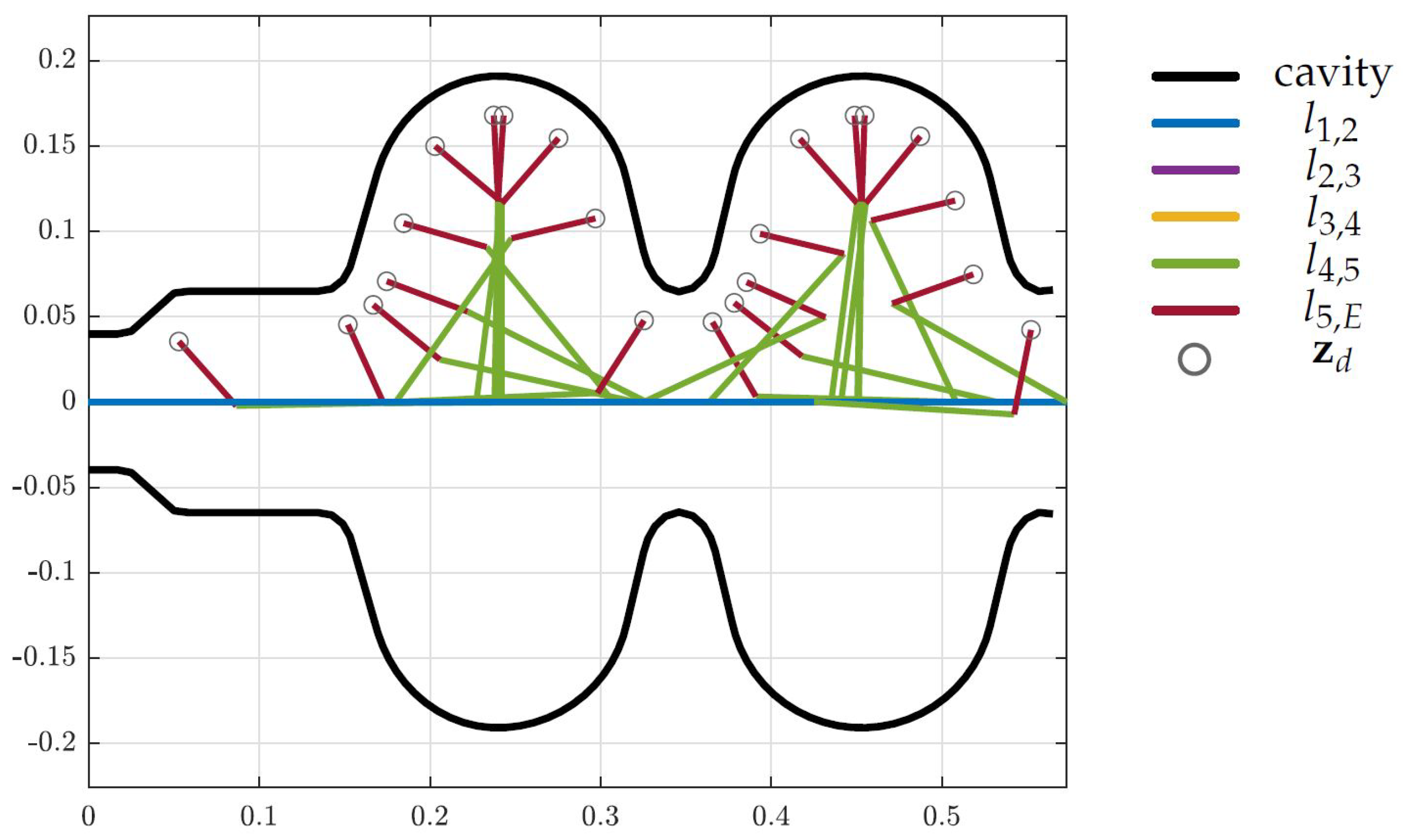
The initial states, such as joint angles and link lengths, heavily influence the performance of optimization algorithms. It is important to provide feasible (in terms of the given constraints) initial states as a starting point for the optimization solvers. Starting points can be generated by either an inverse kinematics method or, as is done here, by running the optimization with the objective function (18) set to . Thus, the initial states are feasible with respect to all constraints, but non-optimal. The initial configurations and link lengths used as a starting point for the optimization solvers are shown for the three cavities in Figure 10, Figure 11 and Figure 12.
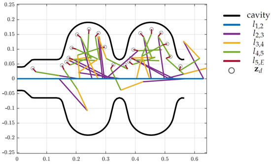
Figure 10.
Initial states for the LINAC cavity (units in m).

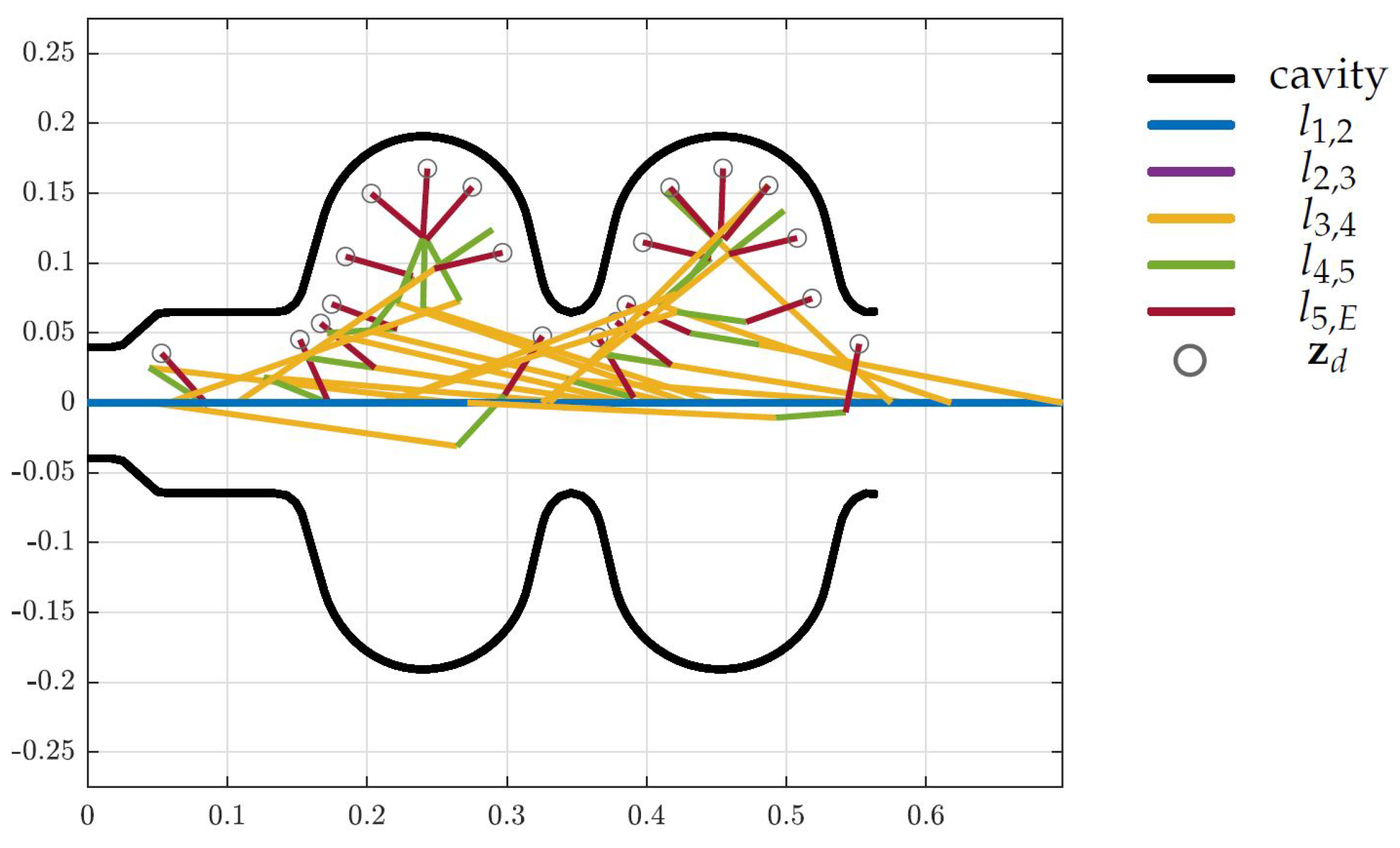
Figure 11.
Initial states for the LHC cavity (units in m).
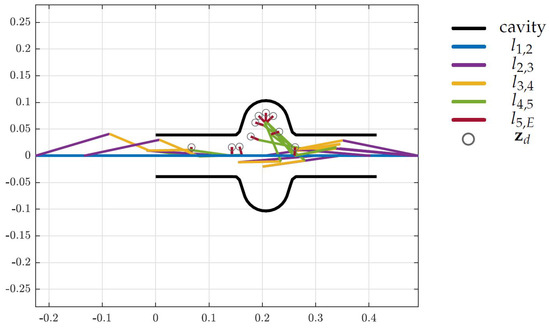
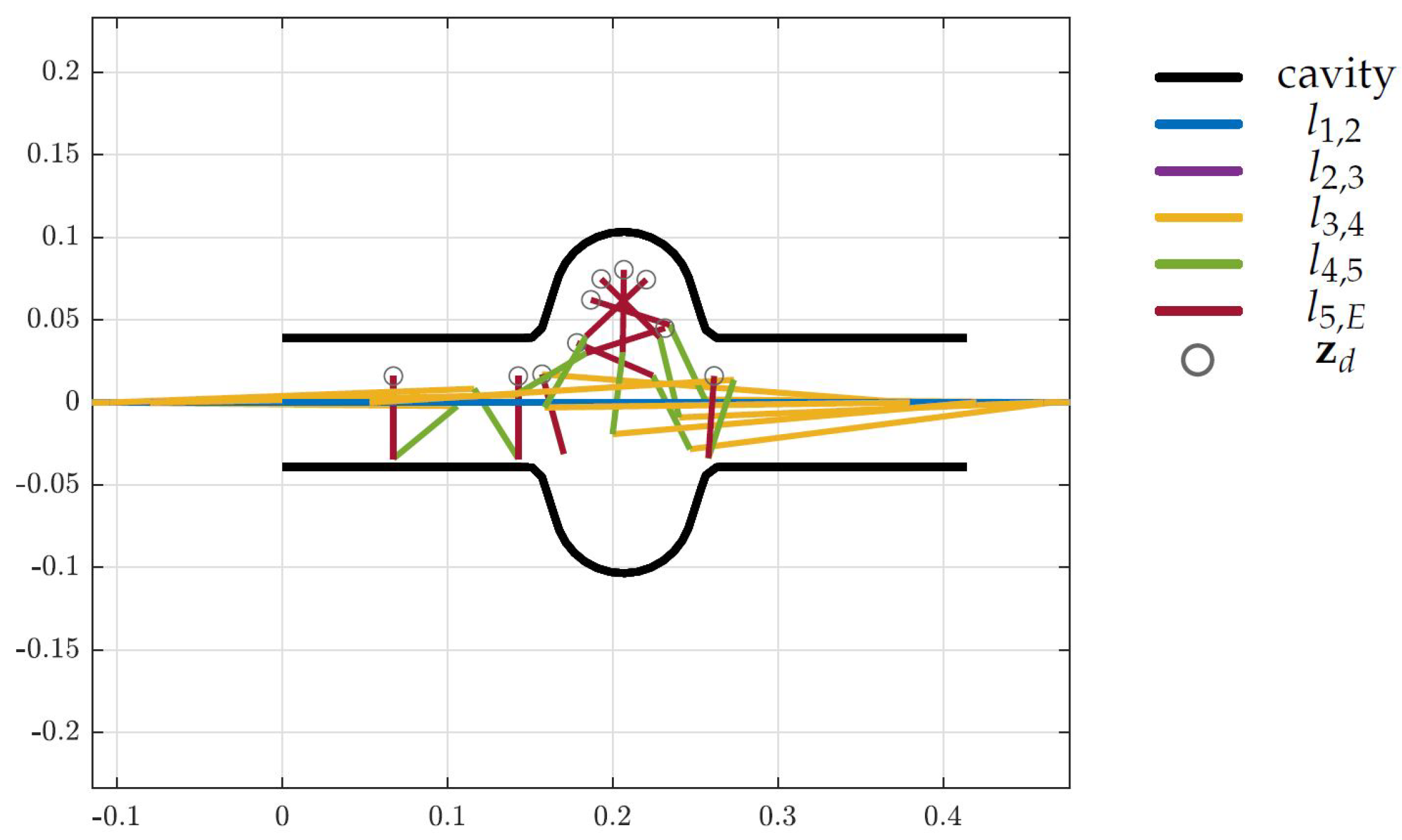
Figure 12.
Initial states for the FCC cavity (units in m).
The black curves represent the cavities and the colored lines represent the robot links. The gray circles indicate the desired end-effector position from vector .
5.5. Optimization Results
The optimization depart from starting points defined for every desired end-effector position and cavity. The starting points have been found by an optimization (described in Section 5.4) and include an initial topology and geometry, as well as the configuration of the arm. Matlab’s fmincon function is internally used as a local optimization solver, in this case, applying the interior-point algorithm [19]. The MultiStart and GlobalSearch methods are applied to solve the global optimization problem [20]. In a comparison with evolutionary algorithms, the GlobalSearch and MultiStart methods leads to better results.
In Section 5.5.1 the design optimization is launched using only the LINAC environment for demonstration purposes and in Section 5.5.2 the robotic arm is optimized to operate in all three cavities.
5.5.1. LINAC Cavity
Here, the design optimization is done only for the LINAC cavity in order to demonstrate the behaviour of the algorithm with a simpler, and, hence, more intuitive example. The initial states match the ones presented in Figure 10 and the corresponding optimized design is visualized in Figure 13.
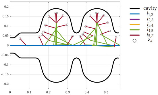
Figure 13.
Optimized design for the LINAC cavity (units in m).
As mentioned in Section 5.1 the desired Cartesian position and orientation is of dimension three and, thus, a mechanical structure with exactly three DoF is able to reach all desired end-effector positions in an environment without obstacles or other constraints. As shown in Figure 13 the restriction caused by the LINAC cavity allows a three-DoF robotic arm to reach all positions. Thus, the optimization reduces the tentative topology by two DoF, which is visible in Figure 14, but more clear in Table 2, where the lengths set to zero correspond to the removed DoF.
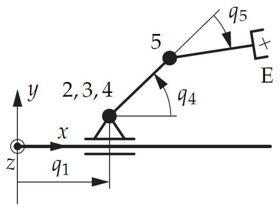
Figure 14.
Optimized topology-LINAC.
Table 2.
Optimized geometry-LINAC.
Furthermore, the length of the robotic arm has been minimized, as becomes clear when looking at the furthest point and observing that all links lie on a straight line from joint 2 to the desired end-effector position, and that this line is perpendicular to the x axis. In Figure 14 the schematic drawing of the optimal topology is shown with some joints coinciding with others and, thus, illustrating the reduction of DoF.
5.5.2. Full System
The design optimization for the full system is performed by considering all three cavities as collision objects in the non-linear inequality constraints of the optimization problem. Again, the results of the optimization are shown in Figure 15, Figure 16 and Figure 17 for the LINAC, LHC and FCC respectively, where the colored lines represent the robot links, the black curves indicate the surface of the cavities and the gray circles show the desired end-effector positions. The resulting topology is shown in Figure 18 and the corresponding link lengths are listed in Table 3.
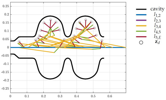
Figure 15.
Optimized design for the LINAC cavity (units in m).
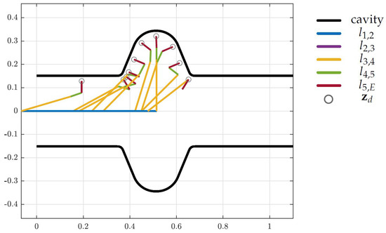
Figure 16.
Optimized design for the LHC cavity (units in m).
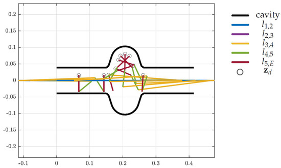
Figure 17.
Optimized design for the FCC cavity (units in m).
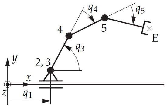
Figure 18.
Optimized topology.
Table 3.
Optimized geometry.
As is clearly visible in Table 3, at least one link length is set to zero, which means that our requirement for the tentative topology of starting the design optimization with at least one DoF higher than the expected optimal solution holds and, thus, an optimized design for the robotic arm has been found.
6. Application: FCC Manipulator
A detailed report on the design optimization of the FCC Manipulator (a robotic system for CERN’s Future Circular Collider) has already been published in [2]. Here, only a brief summary of the assumptions and results are presented to demonstrate the algorithms capabilities.
The Future Circular Collider (FCC) is suggested to unlock observations in higher energy ranges than it is possible, now, with the current accelerator machines at CERN [21]. This particle accelerator is able to generate a center-of-mass energy of 100 TeV and has a planned circumference of 100 km (see [22,23]). The 2020 Update of the European Strategy for Particle Physics has listed the further investigation of the FCC as one of three main priorities and, thus, have launched a Technical Design Report (TDR). One of the studies that has been launched within the TDR concerns the automation of maintenance, inspection and emergency handling along the 100-km-long FCC tunnel. The automation of these tasks plays a significant role for downtime, reliability and safety of particle accelerators and decreases the radiation exposure of workers.
The tasks such an automated system has to handle and the environment it must operate in are well defined, but no restrictions on the actual design of the manipulator in terms of topology and geometry are given. Thus, the presented algorithm has been applied to optimize the tentative design of the FCC robot. In Section 6.1 the model and some assumptions are described. In Section 6.2 the applied objective function, in terms of kinematic and dynamic criteria, is analyzed and finally some results are shown in Section 6.3.
6.1. Manipulator and Environment
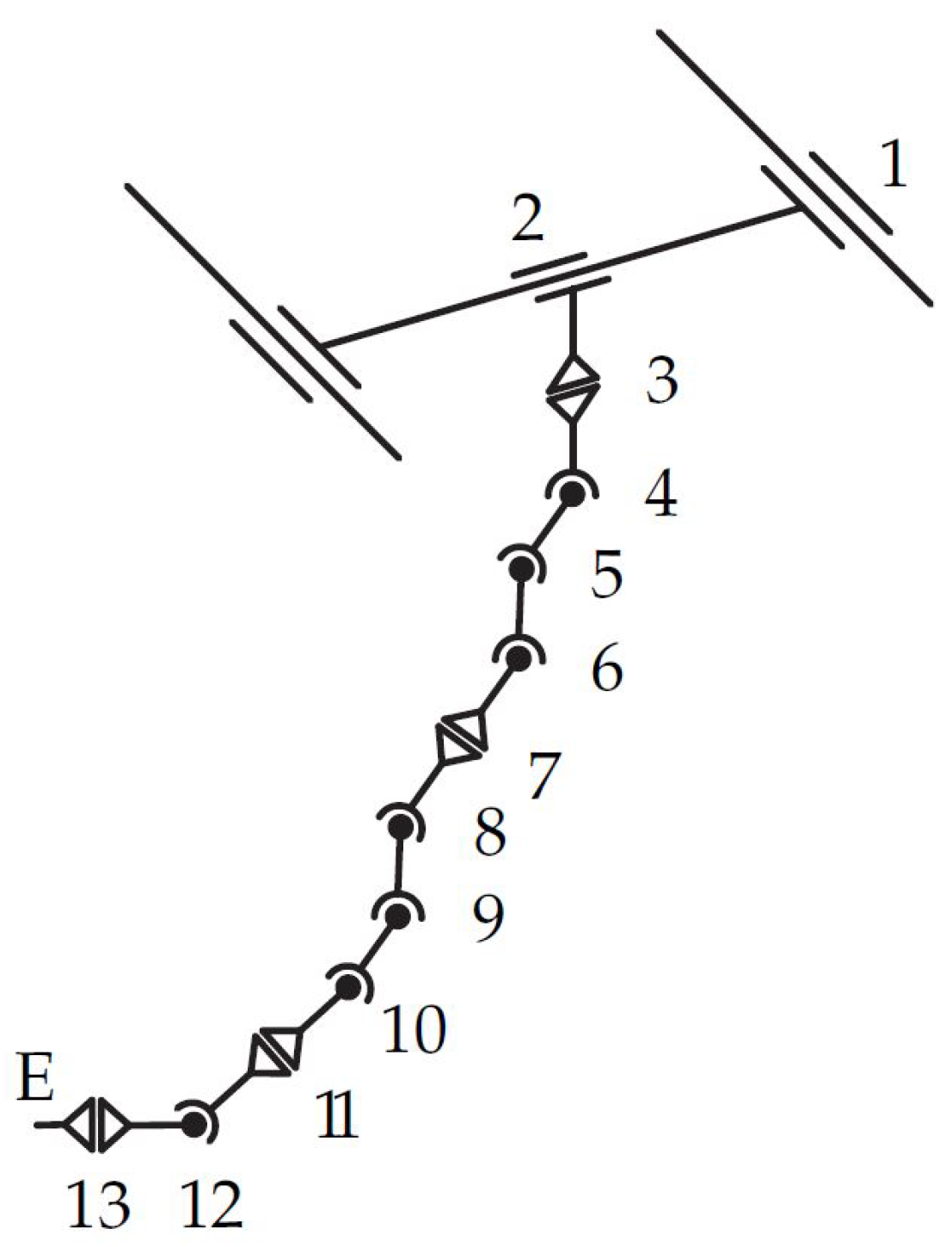
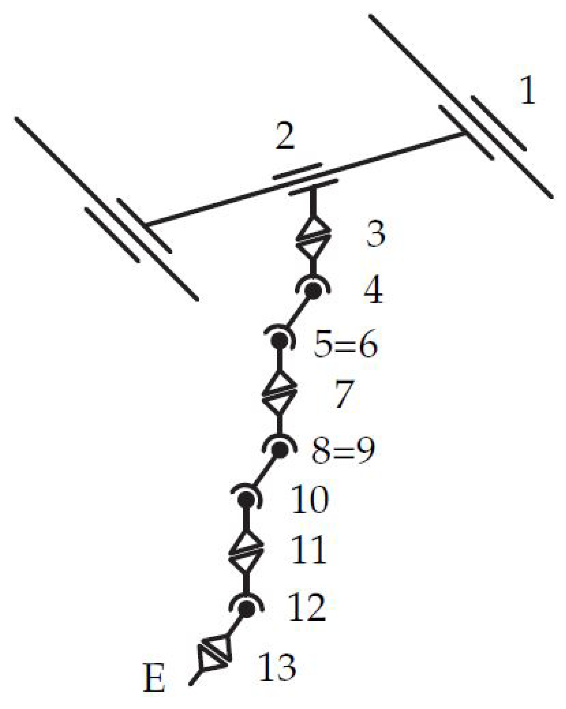
The process of defining the surrogate model, as shown in Figure 19, is described in detail in [2]. Here, it should just be mentioned that joints 1 and 2 are translational joints, 3–6 and 7–10 form two planar mechanisms in order to fold the arm. Joints 11–13 represent a robotic wrist and, thus, the solution for its position and orientation can be decoupled in point 12, which simplifies the optimization problem. The planar chains allow for minimizing the link lengths between joints with parallel axes, and, thus, possibly eliminating joints connected by links with zero length, hence, eventually reducing the DOF. The initial link lengths in Table 4 have been found by the same means as described in Section 5.4.
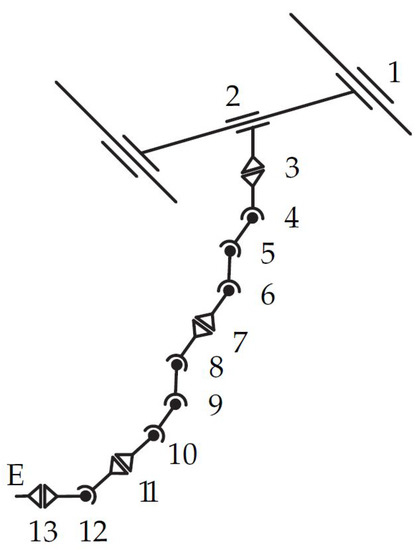
Figure 19.
Design space using VDI2861 (from [2] under CC BY-NC-ND 4.0).
Table 4.
Initial geometry.
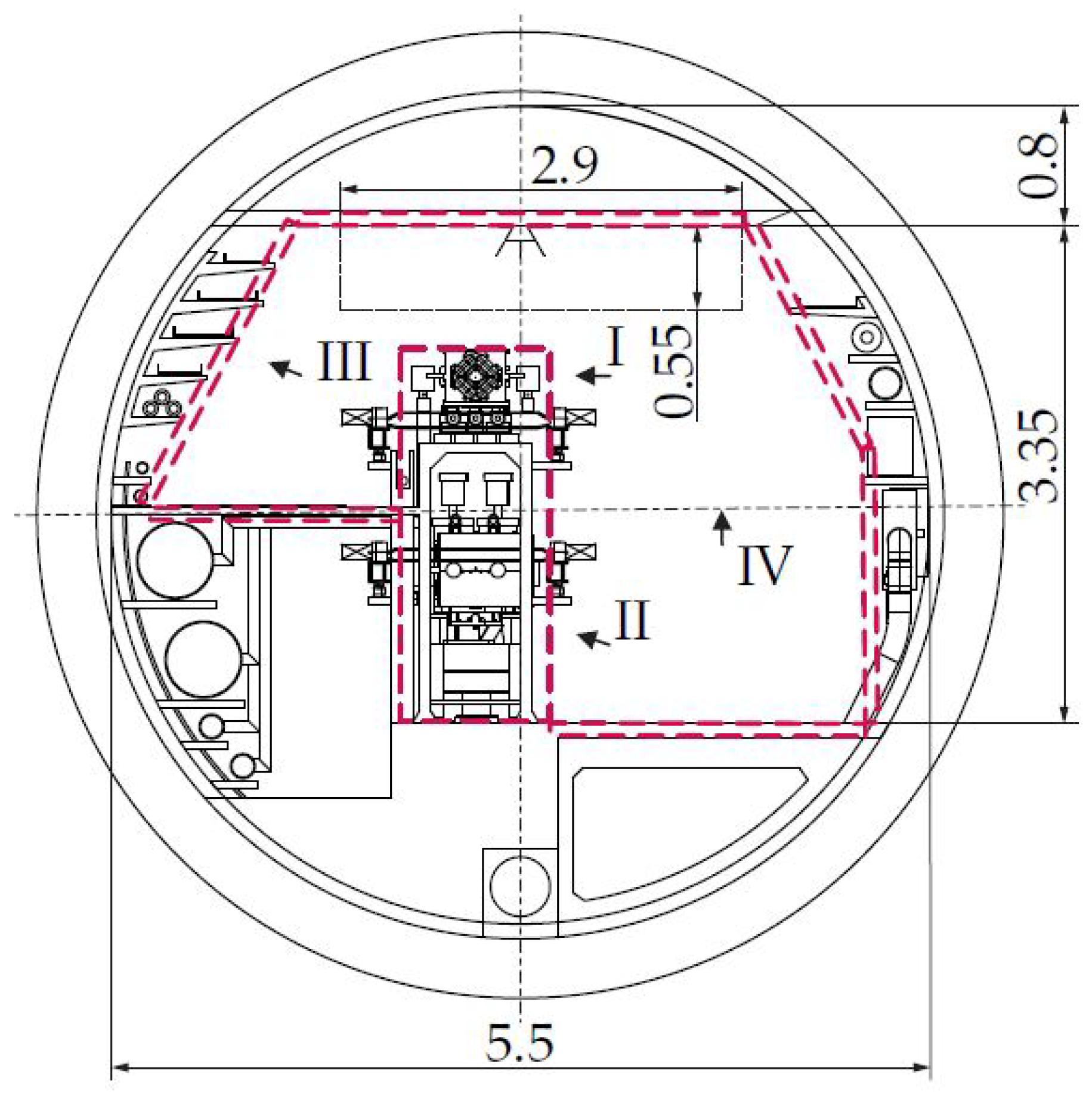
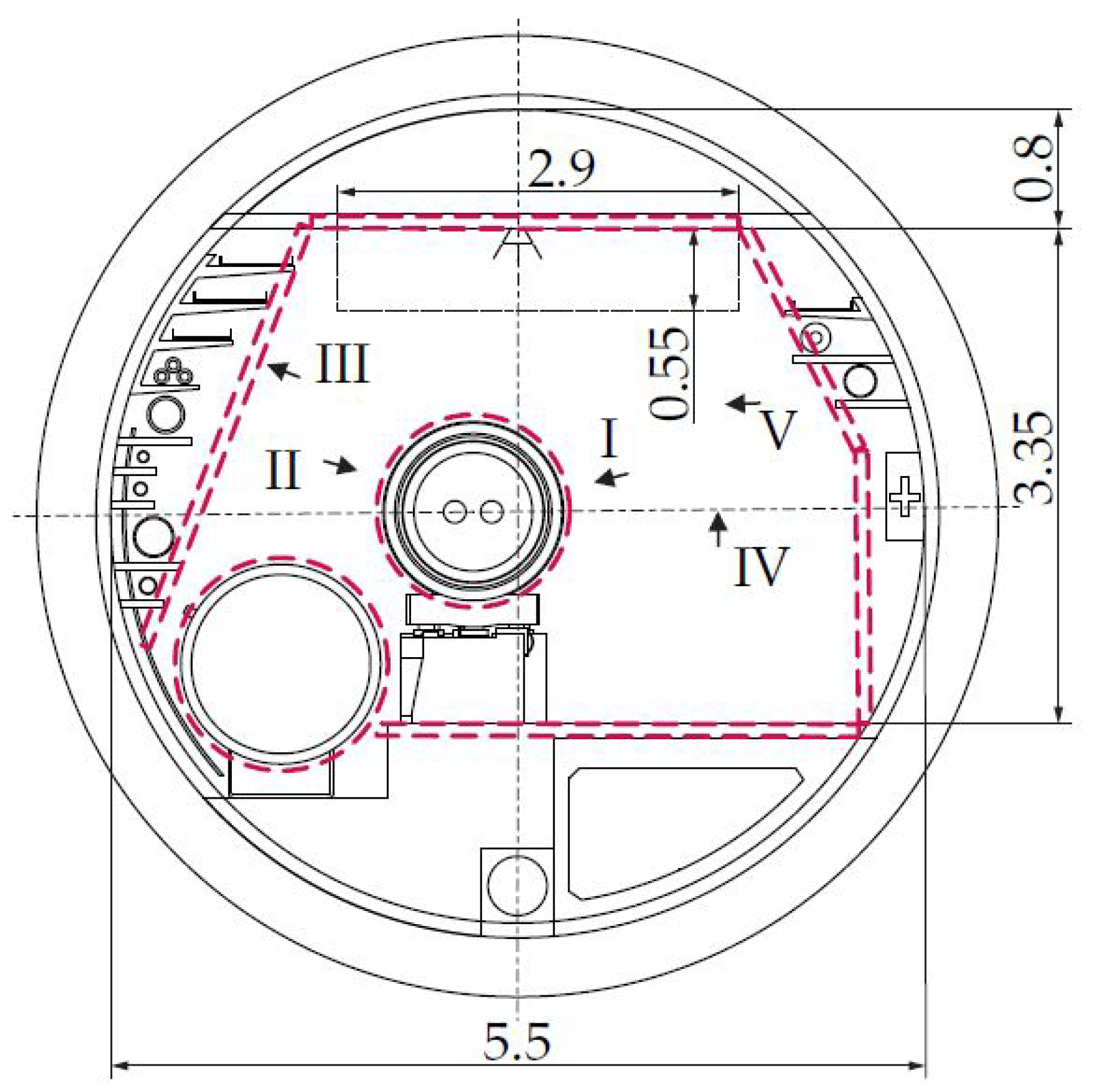
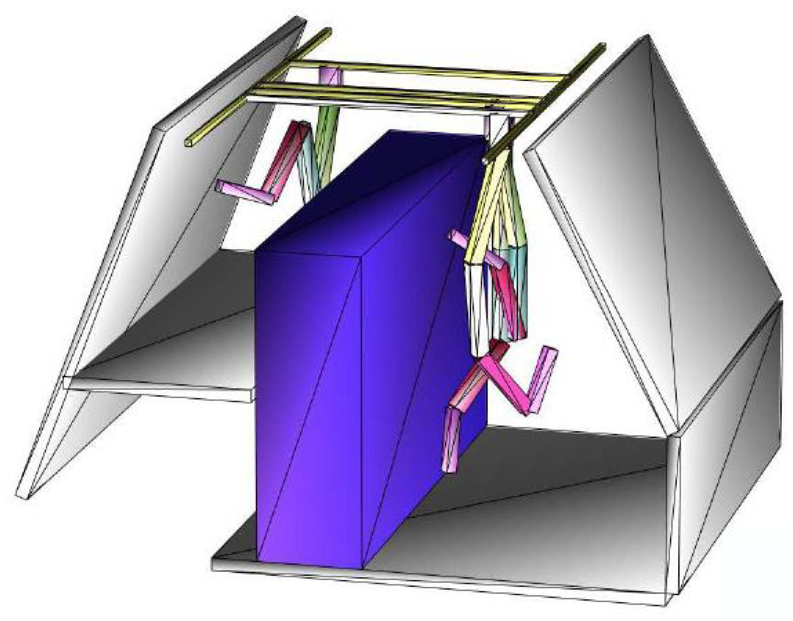
The environment of the FCC tunnel and the robot have been approximated by convex geometric primitives; here, specifically, by Matlab’s AlphaShapes [24], which can easily be passed to a function to calculate the minimal distance between two AlphaShapes. The approximation of the FCC environment with cylinders and boxes is indicated by red, dashed lines in Figure 20 and Figure 21 for the FCC-ee and FCC-hh machines, respectively. The manipulator should be able to reach all points of interest (I–V), which represents the most diverse remote maintenance tasks at the current Large Hadron Collider—LHC, see [25,26,27,28].
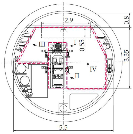
Figure 20.
FCC-ee Cross Section Layout (units in m, from [2] under CC BY-NC-ND 4.0).
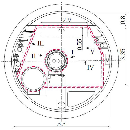
Figure 21.
FCC-hh Cross Section Layout (units in m, from [2] under CC BY-NC-ND 4.0).
6.2. Kinematic and Dynamic Performance Criteria
A main objective for the design of the manipulator is to reduce the motors’ torques, since the workspace, shown in Figure 20 and Figure 21, requires a relatively long robotic arm, compared with the desired payload and weight of the robot. Thus, the dynamic measure applied in term in the objective function (18) is the motor torque of each joint. A dynamic robot model in the form (9) is used and included in the objective function (18) with
and the weighting matrix .
6.3. Optimization Results
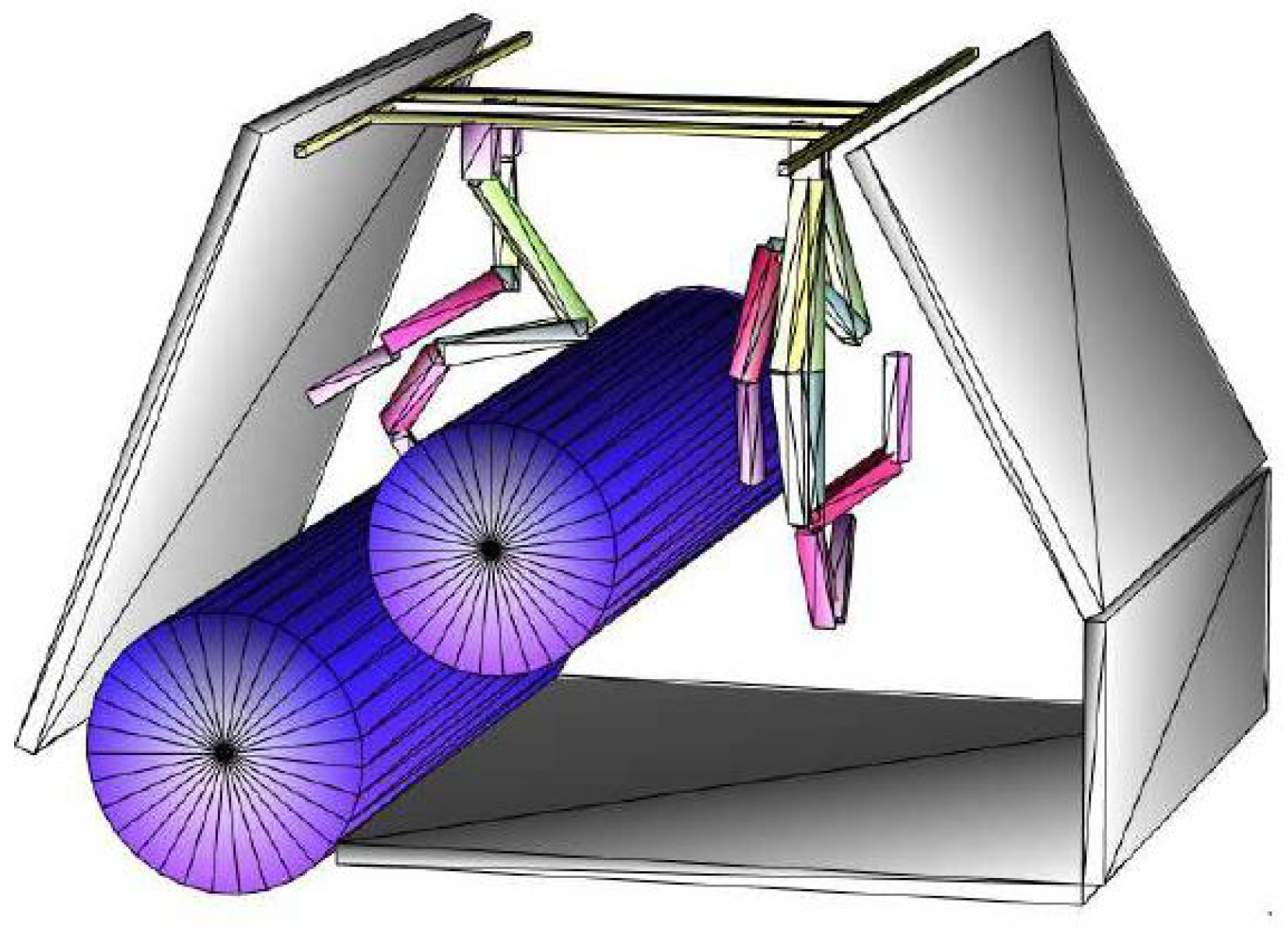
The final results of the design optimization shows a reduced topology by two DoF. This is shown in Figure 22 by the coinciding joints 5/6 and 8/9, which correspond to the lengths in Table 5 of the optimized geometry. In Figure 23 and Figure 24 the optimization results are visualized using the collision objects (AlphaShapes) for the two different accelerator machines, FCC-ee and FCC-hh.
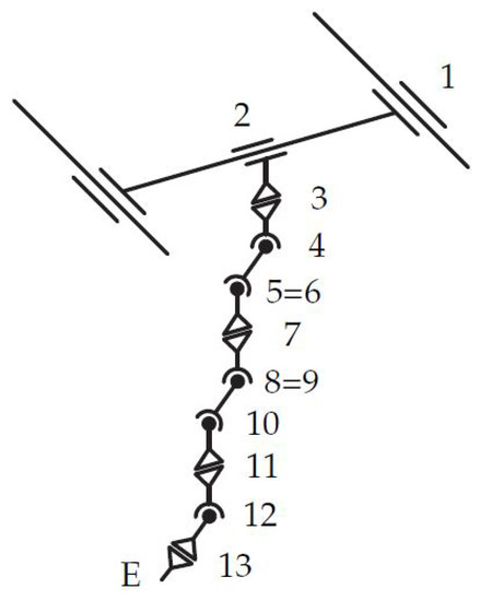
Figure 22.
Optimized topology using VDI2861 (from [2] under CC BY-NC-ND 4.0).
Table 5.
Optimized geometry.

Figure 23.
Optimization results FCC-ee (from [2] under CC BY-NC-ND 4.0).
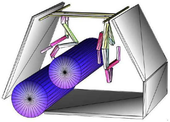
Figure 24.
Optimization results FCC-hh (from [2] under CC BY-NC-ND 4.0).
7. Discussion and Conclusions
A kinematic model pruning method has been presented that allows transforming discrete optimization criteria into a continuous representation and, thus, enables simultaneous optimization of the topology and geometric parameters. The method has been demonstrated for serial mechanical structures and, therefore, covers a wide variety of robotic manipulators. The algorithm uses well-known and readily available optimization schemes without any additional, complex frameworks. The simplicity of the presented kinematic model pruning method is surely one of its main advantages, next to the simultaneous optimization of all additional criteria. It is especially simple, since no inverse kinematics are computed and, for the case without additional dynamic performance criteria, no dynamic model is needed. Thus, this method can be performed providing only the forward kinematics and (if necessary) collision detection. This allows for very quick prototyping and one does not have to rely on either complex frameworks or an “educated guess” for a new manipulator design, but, instead, can quickly produce quantified results based on deterministic performance criteria. As demonstrated with examples in Section 5 and Section 6, the algorithm has led to good results for both the cavity inspection arm and the FCC Manipulator.
The choice of additional kinematic and dynamic criteria needs to be made carefully in order to not generate ill-conditioned optimization problems or even contradictions with the requirements. The weighting matrices in (18) have a major impact on the final results and can, as well, lead to infeasible solutions, in certain cases. Finding guidelines for these optimization parameters based on the mechanical structure and environment would simplify this heuristic process. The current implementation only allows for DoF reduction on two subsequent joints of the same type. An extension of the presented method to a more general use case, including closed kinematic chains, will be the subject of future work. Furthermore, a more general study on stability, convergence rates and the effects of different optimization schemes applying the proposed pruning function will be investigated.
Author Contributions
Formal analysis, H.G. (Hannes Gamper); Methodology, H.G. (Hannes Gamper); Supervision, H.G. (Hubert Gattringer), A.M. and M.D.C.; Validation, A.L.; Writing—original draft, H.G. (Hannes Gamper) and A.M. All authors have read and agreed to the published version of the manuscript.
Funding
This research received no external funding.
Institutional Review Board Statement
Not applicable.
Informed Consent Statement
Not applicable.
Conflicts of Interest
The authors declare no conflict of interest.
Abbreviations
The following abbreviations are used in this manuscript:
| DoF | degrees of freedom |
| LHC | Large Hadron Collider |
| LINAC | linear accelerator |
| RF | radio frequency |
| FCC | Future Circular Collider |
| FCC-ee/-hh | Future Circular Collider-lepton/-hadron machine layout |
References
- Luthi, A.; Macpherson, A.; Rosario Buonocore, L.; Gamper, H.; DiCastro, M. Camera Placement in a Short Working Distance Optical Inspection System for RF Cavities. In Proceedings of the International Conference on RF Superconductivity, Virtual Conference, 28 June–2 July 2021. [Google Scholar]
- Gamper, H.; Gattringer, H.; Müller, A.; Di Castro, M. Design Optimization of a Manipulator for CERN’s Future Circular Collider (FCC). In Proceedings of the 18th International Conference on Informatics in Control, Automation and Robotics—ICINCO 2021, Online, 6–8 July 2021; pp. 320–329. [Google Scholar] [CrossRef]
- Kelaiaia, R.; Company, O.; Zaatri, A. Multiobjective optimization of a linear Delta parallel robot. Mech. Mach. Theory 2012, 50, 159–178. [Google Scholar] [CrossRef]
- Bi, Z.M.; Zhang, W.J. Concurrent optimal design of modular robotic configuration. J. Robot. Syst. 2001, 18, 77–87. [Google Scholar] [CrossRef]
- Henry, R.; Chablat, D.; Porez, M.; Boyer, F.; Kanaan, D. Multi-Objective Design Optimization of the Leg Mechanism for a Piping Inspection Robot. In Proceedings of the 38th Mechanisms and Robotics Conference, Buffalo, NY, USA, 17–20 August 2014; Volume 5A. [Google Scholar] [CrossRef] [Green Version]
- Van Henten, E.; Van’t Slot, D.; Hol, C.; Van Willigenburg, L. Optimal manipulator design for a cucumber harvesting robot. Comput. Electron. Agric. 2009, 65, 247–257. [Google Scholar] [CrossRef]
- Lum, M.J.; Rosen, J.; Sinanan, M.N.; Hannaford, B. Kinematic optimization of a spherical mechanism for a minimally invasive surgical robot. In Proceedings of the IEEE International Conference on Robotics and Automation, New Orleans, LA, USA; 26 April–1 May 2004; Volume 2004, pp. 829–834. [Google Scholar] [CrossRef]
- Schappler, M.; Ortmaier, T. Dimensional Synthesis of Parallel Robots: Unified Kinematics and Dynamics using Full Kinematic Constraints. In Proceedings of the Sechste IFToMM D-A-CH Konferenz 2020, Lienz, Austria, 27–28 February 2020; Volume 2020. [Google Scholar] [CrossRef]
- Rodriguez, D.A.R. Automatic Generation of Task-Specific Serial Mechanisms Using Combined Structural and Dimensional Synthesis; Institutionelles Repositorium der Leibniz Universität Hannover: Hannover, Germany, 2018. [Google Scholar] [CrossRef]
- Ha, S.; Coros, S.; Alspach, A.; Kim, J.; Yamane, K. Computational co-optimization of design parameters and motion trajectories for robotic systems. Int. J. Robot. Res. 2018, 37, 1521–1536. [Google Scholar] [CrossRef]
- Whitman, J.; Choset, H. Task-Specific Manipulator Design and Trajectory Synthesis. IEEE Robot. Autom. Lett. 2019, 4, 301–308. [Google Scholar] [CrossRef]
- CERN. Accelerating: Radiofrequency Cavities. Available online: https://home.cern/science/engineering/accelerating-radiofrequency-cavities (accessed on 2 December 2021).
- Watanabe, K. Review of optical inspection methods. In Proceedings of the 14th International Conference on RF Superconductivity, Berlin\Dresden, Germany, 20–25 September 2009. [Google Scholar]
- Wenskat, M. Automated optical inspection and image analysis of superconducting radio-frequency cavities. J. Instrum. 2017, 12, 1–10. [Google Scholar] [CrossRef] [Green Version]
- Lemke, M.; Elsen, E.; Aderhold, S.; Cornett, U.; Falley, G.; Karstensen, S.; Külper, T.; Navitski, A.; Schaffran, J.; Schlander, F.; et al. Optical Bench for Automated Cavity Inspection with High Resolution on Short Time Scales. ILC-HiGrade-Reports 2013. Available online: https://bib-pubdb1.desy.de/record/166454/files/ILC-HiGrade-2013-001-1.pdf?version=1 (accessed on 14 December 2021).
- Iwashita, Y.; Tajima, Y.; Hayano, H. Development of High Resolution Camera for Observations of Superconducting Cavities. Rev. Mod. Phys. Sept. 2008. [Google Scholar] [CrossRef] [Green Version]
- Gattringer, H. Starr-Elastische Robotersysteme; Springer: Berlin/Heidelberg, Germany, 2011. [Google Scholar]
- Nait-Chabane, K.; Hoppenot, P.; Colle, E. Directional Manipulability for Motion Coordination of an Assistive Mobile Arm. In Proceedings of the 4th International Conference on Informatics in Contronl, Automation and Robotics, Angers, France, 9–12 May 2007. [Google Scholar]
- Byrd, R.H.; Hribar, M.E.; Nocedal, J. An Interior Point Algorithm for Large-Scale Nonlinear Programming. SIAM J. Optim. 1999, 9, 877–900. [Google Scholar] [CrossRef]
- Ugray, Z.; Lasdon, L.; Plummer, J.; Glover, F.; Kelly, J.; Marti, R. Scatter Search and Local NLP Solvers: A Multistart Framework for Global Optimization. INFORMS J. Comput. 2007, 19, 328–340. [Google Scholar] [CrossRef]
- CERN. Future Circular Collider (FCC). Available online: https://home.cern/science/accelerators/future-circular-collider (accessed on 8 December 2021).
- CDR. FCC-ee: The Lepton Collider. Eur. Phys. J. Spec. Top. 2019, 228, 261–623. [Google Scholar] [CrossRef]
- CDR. FCC-hh: The Hadron Collider. Eur. Phys. J. Spec. Top. 2019, 228, 755–1107. [Google Scholar] [CrossRef]
- The MathWorks Inc., Matlab Version 2019, Computer software. Available online: https://ch.mathworks.com/ (accessed on 10 July 2021).
- Bestmann, P. CERN The Control of the LHC Alignment Using a Robot, CERN-TS-NOTE-2008-020. May 2008. Available online: https://cds.cern.ch/record/1119514 (accessed on 2 December 2021).
- Missiaen, D.; Steinhagen, R.; Quesnel, J. The Alignment of the LHC. In Proceedings of the 23rd Particle Accelerator Conference, Vancouver, BC, Canada, 4–8 May 2009. [Google Scholar]
- Valentino, G.; Aßmann, R.; Bruce, R.; Redaelli, S.; Rossi, A.; Sammut, N.; Wollmann, D. Semiautomatic beam-based LHC collimator alignment. Am. Phys. Soc. 2012, 15, 051002. [Google Scholar] [CrossRef]
- Bajko, F.B.M. Report of the Task Force on the Incident of 19 September 2008 at the LHC; LHC Project Report 1168; 2009. Available online: https://inspirehep.net/literature/824814 (accessed on 2 December 2021).


Publisher’s Note: MDPI stays neutral with regard to jurisdictional claims in published maps and institutional affiliations. |
© 2022 by the authors. Licensee MDPI, Basel, Switzerland. This article is an open access article distributed under the terms and conditions of the Creative Commons Attribution (CC BY) license (https://creativecommons.org/licenses/by/4.0/).