Article

Collision Avoidance for Redundant 7-DOF Robots Using a Critically Damped Dynamic Approach

by
Henrique Simas
1 and
Raffaele Di Gregorio
2,*
1
Raul Guenther Lab. of Applied Robotics, Department of Mechanical Engineering, Federal University of Santa Catarina, Florianópolis 88040-900, Brazil
2
Lab. of Mechatronics and Virtual Prototyping (LaMaViP), Department of Engineering, University of Ferrara, Via Saragat,1, 44100 Ferrara, Italy
*
Author to whom correspondence should be addressed.
Robotics 2022, 11(5), 93; https://doi.org/10.3390/robotics11050093
Submission received: 23 July 2022 / Revised: 30 August 2022 / Accepted: 4 September 2022 / Published: 8 September 2022
(This article belongs to the Special Issue Kinematics and Robot Design V, KaRD2022)

Abstract

:
The presence of collaborative robots in industrial environments requires that their control strategies include collision avoidance in the generation of trajectories. In general, collision avoidance is performed via additional displacements of the kinematic chain that make the robot move far from the objects that are occasionally inserted into its safety workspace. The variability of the coordinates of the collision points inside the safety volume leads to abrupt movements for the robot. This paper presents a general method for smoothing abrupt movements in robots with one degree of redundancy for collision-avoidance trajectories, employing a second-order digital filter designed with adjustable critical damping. The method is illustrated by applying it to a redundant robot with a spherical–revolute–spherical type (SRS-type) kinematic chain, which is a benchmark used to test the algorithms ideated for solving this problem. This paper also presents an alternative algorithm for the inverse kinematics of the SRS-type robot and the computational experiments that show the collision avoidance proposal’s performance and its properties through graphical results.

1. Introduction

Complex tasks require interactions between robots and humans collaboratively. This collaboration comes from sharing tools, operations, and workspaces [1,2,3] and requires specific control techniques to overcome possible collisions between robots and humans or devices located inside the workspace [4]. Such collaboration implies a more significant number of restrictions on the volume available to the end-effector and the respective safety volume (i.e., the geometric spatial volume around the links and the end-effector, where the robot is considered free of collisions) available for the displacements of the robot’s kinematic chain [5]. In this sense, a new class of robots is arising, defined as collaborative robots [6,7], which are provided with strategies at the hardware and software levels to avoid collisions and improve the interactions between robots and humans. Collision-avoidance strategies require additional movements of the kinematic chains, which means that the robots need to have greater mobility than what is needed to perform their tasks; that is, they need to be redundant [6,8,9,10,11]
Elements inserted into a robot’s safety workspace [12] usually make the robot change its coordinates randomly, causing abrupt variation in the distances to the points belonging to the robot’s kinematic chain. If the values of these distances are used as references in collision-avoidance algorithms, the movements of the robot’s kinematic chain are abrupt and naturally undesirable. Indeed, abrupt changes in joint variables, besides being physically difficult to obtain, generate vibrations in a wide range of frequencies that cannot be tolerated during machine motion. This is why smoothing the additional motion that avoids a possible collision is an important requirement for any collision-avoidance strategy.
Collision-avoidance strategies consist of programming a set of internal movements of a robot’s kinematic chains based on sensor data to circumvent or deviate certain parts of the robot from an obstacle that has been inserted into its overall workspace, which can occur in online, offline, or autonomous tasks [3,4,12]. The internal movements are performed via changes in joint displacements, which often lead to abrupt variations in joint trajectories [13,14] and need to be treated to ensure smooth movement.
Improving the motion quality requires collision-avoidance strategies that generate smooth transients in terms of joint displacements and rates. Such strategies are, in general, based on optimization algorithms via energy minimization [15,16] or on differential geometric approaches [8,17,18], which, among other propositions, are based on the Moore–Penrose pseudoinverse approach [19,20] and are limited mainly by the problem of homogeneity and the lack of repeatability of the solutions [21,22]. A systematic proposition based on concepts of linear equations independent of numerical optimization methods [23] allows for better control over the performance and execution of the collision-avoidance strategy.
Some interesting trajectory generation proposals involve using digital filters in the definition of reference signal limits [24,25] or combined with curve formulations [26,27]. The complexity and limited adjustment possibilities make it difficult to replicate or use such strategies, limiting their application. The aim of this work is to overcome these applicative limitations.
This paper presents a new approach to collision avoidance based on the use of second-order digital filters [28], which solves the inverse kinematics through the resolved motion control technique (RMC) [14,29]. The proposal calculates the minimum distance straight line between the nearest collision point of a mobile obstacle and the robot’s links using a geometric formulation. The length of this straight-line segment changes as the collision point coordinates change inside the robot’s overall workspace. The collision-avoidance algorithm proposition calculates the internal movements (null space of the kinematic chain [30,31]), smoothing abrupt movements that eventually arise. The proposal uses a low-pass filter to minimize the possible peaks of the internal displacements, improving the transients of the trajectory in the kinematic chain while the robot executes a task. The proposal also considers an envelope defined by a geometric surface around the links as a safety region and obtains a smooth transition through a digital filter, which allows adjustments according to the desired performance and response-time criteria [21,22,28].
Several spherical–revolute–spherical-type (SRS-type) redundant robots have arisen as workbenches for the simulation and experimentation of such proposals [5,15,26,32,33,34], including the arms or legs of bipedal robots [33,35,36,37]; among these, the Kuka-LBR-iiwa models are the most adopted SRS-type redundant robots [8,9,11,38,39]. The experimentation on the proposed collision-avoidance strategy uses the Kuka-LBR-iiwa’s kinematic model with seven degrees-of-freedom (DOFs), which is commonly used to test collision-avoidance strategies in collaborative cells [4,7,8,27]. Such a choice will allow comparisons and a more accurate assessment of the proposition’s advantages.
Here, the proposed strategy is proven and discussed using a simulation experiment, where the collision-avoidance control acts to avoid the collisions between the links of the SRS-type redundant robot and two kinematic models of human arms that share the robot’s safety volume [12] while performing tasks in an industrial simulation environment.
This paper is organized as follows. Section 2 presents the proposed collision-avoidance strategy. Section 3 presents the SRS-type redundant robot benchmark and a proposal for solving its inverse kinematics. Section 4 presents the new approach for defining the safe region around the links and calculating the distance between a point and the robot. Section 5 presents the graphical results, and Section 6 discusses the results. Finally, Section 7 draws the conclusions.

2. Critically Damped Collision Avoidance

Let Pc be a point with an imminent possibility of collision with a redundant robot. Such a point may belong to a human operator or to another apparatus occasionally inserted into the robot’s safety volume [12,40,41]. The collision-avoidance strategy must avoid the collision by acting in the null space of a redundant robot so that the robot’s configuration changes using movements, chosen according to the degree of redundancy [11,30], that do not affect the task performed by the robot. In short, without redundancy, avoiding a possible collision can be achieved only by changing the motion task of the robot.
The collision-avoidance method proposed in this paper holds for robots with only one degree of redundancy. So, we can only exploit a movement with one DOF to avoid a collision. In the literature, for the case of the SRS-type redundant robot of Figure 1, which is a benchmark for this problem, angle α is usually chosen for controlling the distance between the elbow point Pe and the collision point Pc using criteria such as geometric approaches [1,38], differential maps [17,29], and energy [5,25,26,32]. The problem reduces itself to ideate an inverse-kinematics algorithm that makes angle α perform the internal movements (null-space) of the kinematic chain without changing the position and orientation of the end-effector.
From a geometric point of view, the problem consists of verifying the minimum distance, dmin, between the robot and the nearest point, Pc, of a mobile obstacle and then adjusting the value of angle α to guarantee a minimum desired distance, drmin. Considering that point Pc may change its coordinates randomly or abruptly in the space at each measurement of its coordinates (e.g., obtained through sensors or video cameras [42]), the respective change of angle α may produce abrupt oscillations of the joint positions, calculated with inverse-kinematics algorithms, which is an undesirable and often, unpractical result.
To avoid abrupt oscillations in the values of the joint positions, it is interesting to smooth angle-α transients before using them as input data for the inverse-kinematics algorithms. Smoothing improves continuity in signal transitions and variations based on polynomial numerical interpolations [43]. Such an approach has limitations when the order of signals’ derivatives is greater than polynomials’ order; indeed, in this case, continuity is no longer guaranteed.
This work proposes that angle α be numerically filtered by using a time-continuous second-order transfer function, G(s), defined as follows, which is critically damped and has a static gain equal to 1 [28]:
α f ( s ) α c ( s ) = G ( s ) = p 2 ( s + p ) 2
In Equation (1), αc(s) corresponds to a time-continuous signal input for the α values on the complex s-domain calculated to avoid the collision; αf(s) is the respective continuous output, signal-filtered; and p is an adjustable pole, which allows setting the speed of the transients [28]. The critically damped dynamics consist of second-order systems that have a time response with faster transients without overshoot, where the damping coefficient ξ = 1 [28].
Using the filtered signal, αf, in a trajectory-generator algorithm needs the discretization of the transfer function, G(s), defined by Equation (1). The discretization of G(s) is given by its z-transform associated with a zero-order hold (ZOH) [28] as follows:
α f ( s ) α c ( s ) = G ( z ) = 1 z 1 Z G ( s ) s = ( 1 e m ( 1 + m ) ) z 1 + e m ( m 1 + e m ) z 2 1 2 e m z 1 + e 2 m z 2 = h 1 z 1 + h 2 z 2 1 b 1 z 1 b 2 z 2
where T is the desired sample time (in general defined as a function of the computer clock, or interfaces sample times); m is the product Tp; h1 = (1 − em(1 + m)); h2 = em (m – 1 + em); b1 = 2em; and b2 = −e2m.
Using the right-shift or delay theorem [28], the variable z behaves like a delay operator for the input and output variables of the discrete transfer function presented in Equation (2). In this way, it is possible to obtain a command line for the algorithm that filters the α angle as follows:
α f ( n ) = h 1 α c ( n 1 ) + h 2 α c ( n 2 ) + b 1 α f ( n 1 ) + b 2 α f ( n 2 )
where “n” is the discrete parameter, that is, n = 0, 1, …, whereas α c and α f are the computed-input and the filtered-output angle α calculated at the instant “n”, respectively. It is worth noting that since the signal starts at n = 0, it is necessary to define the initial conditions of α f and α c for n = 2 , 1 .

3. SRS-Type Redundant Robot Benchmark

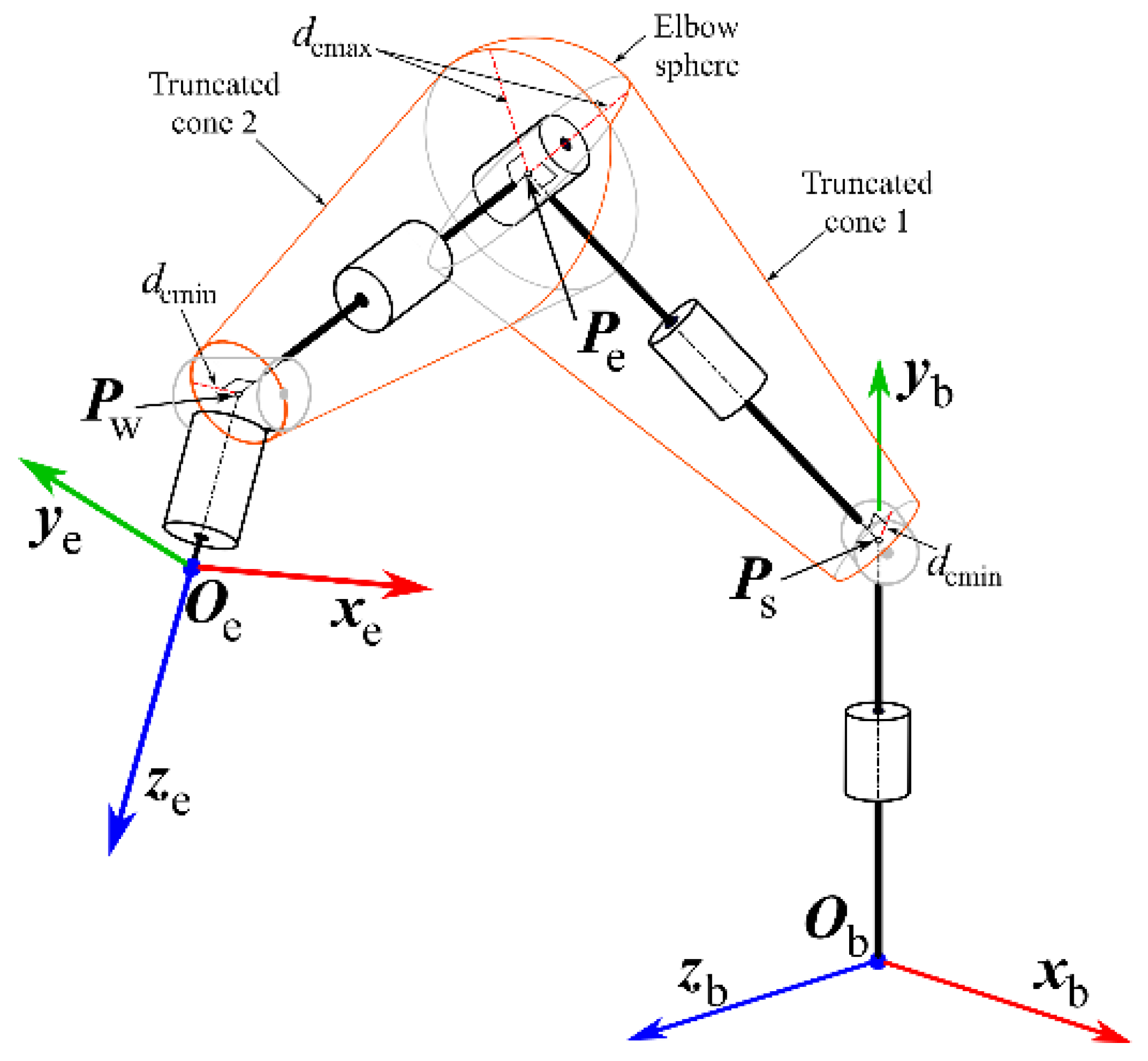
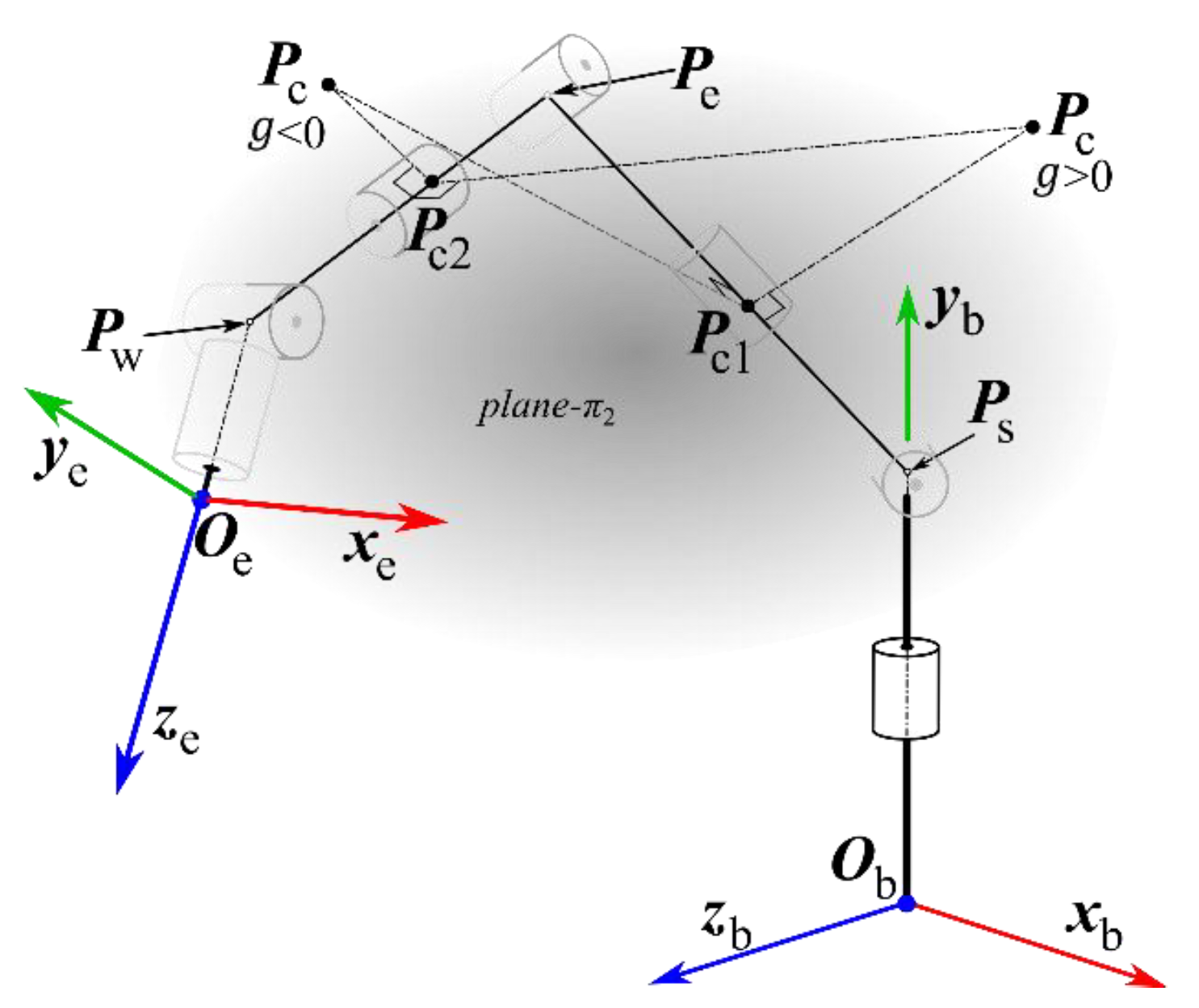
3.1. Geometric Description

The SRS-type robot is a redundant robot with seven revolute joints (7-DOF) with the possibility of elbow movement, adapted mainly for collaborative tasks between robots or robots and humans [9,44,45]. The scope of applications has encouraged several authors to develop research and proposals for the kinematic modeling of this robot [8,9,26,35,37,46]. A typical SRS-type redundant robot is the Kuka-LBR-iiwa [4,44], whose kinematic model is shown in Figure 1.
With reference to Figure 1, the links are numbered from 0 (the frame) to 7 (the end effector), and the revolute(R)-joint variables are q = [ θ 1 θ 2 θ 3 θ 4 θ 5 θ 6 θ 7 ] T (see Figure 1a), whereas the constant lengths are a = [ a 0 a 1 a 3 a 4 ] T (see Figure 1b). Link 0 is the frame (base), and the Cartesian reference Ob-xbybzb is fixed to the base, whereas link 7 is the end-effector and the Cartesian reference Oe-xeyeze is fixed to the end effector. Here, without losing generality, for the sake of simplicity, the assumption that the tool is displaced a3 from the center of the spherical wrist is introduced. The seven R-joints are numbered from 1 to 7 following the order they are encountered by moving from the base to the end effector along the 7R kinematic chain of the robot.
The 7-DOF Kuka-LBR-iiwa robot is a serial chain of SRS-type. Indeed, the axes of the first three R-joints, with joint variables (θ1, θ2, θ3), intersect at Ps, which is the center of the first S-pair, and the axes of the last three R-joints, with joint variables (θ5, θ6, θ7), intersect themselves at Pw, which is the center of the second S-pair (i.e., the wrist of the robot). The axis of the first R-joint coincides with the yb-axis, whereas the axis of the second R-joint is perpendicular to the yb-axis and passes through Ps. The axis of the third R-joint is perpendicular to both the axes of the second and the fourth R-joints and intersects the axis of the fourth R-joint at Pe. Points Ob, Ps, and Pw lie on a plane, hereafter named plane-π1, which contains the yb-axis. Points Ps, Pe, and Pw lie on another plane, hereafter named plane-π2, whose normal is parallel to the axis of the fourth R-joint. The axis of the fifth R-joint passes through Pe, is perpendicular to both the axes of the fourth and the sixth R-joints, and intersects the axis of the sixth R-joint at Pw: θ 5 is the angle between the axes of the fourth and the sixth R-joints. Eventually, the axis of the seventh R-joint passes through Pw and is perpendicular to the axis of the sixth R-joint: θ6 is the angle between the axes of the fifth and the seventh R-joints.
The constant lengths, shown in Figure 1b, are defined as follows: a0 is the distance between points Ob and Ps; a1 is the distance between points Ps and Pe; a2 is the distance between points Pe and Pw; and a3 is the distance between points Pw and Oe. In addition, three characteristic internal points are defined (see Figure 1b): Psshoulder point—in the center of the first S-pair; Peelbow point—in the crossing point of the joint axes 3, 4, and 5; and, lastly, Pw in the center of the second S-pair (the robot wrist). When θ 3 = 0 rad, the points Ob, Ps, Pe, and Pw belong to the same plane (i.e., plane-π1 and plane-π2 coincide with one another), making the kinematic chain like a classical 6-DOF anthropomorphic robot. Differently, when θ 3 0 rad, point Pe goes out of plane-π1, and the line passing through points Ps and Pw becomes the common intersection between plane-π1 and plane-π2, which Pe lies on. The angle α between these two planes (see Figure 1b) can be chosen as the seventh generalized coordinate that, together with the coordinates bp7 = [x7 y7 z7]T of point Pw in Ob-xbybzb and the end-effector’s orientation parameters bφe = [φe ϑe ψe ]T with respect to Ob-xbybzb, uniquely identifies the configuration of the 7-DOF robot in the operational space.
From a geometric point of view, angle α is a rotation angle around the line segment PsPw. In short, we have x = [bp7T bφeT α] T as operational-space coordinates and q = [ θ 1 θ 2 θ 3 θ 4 θ 5 θ 6 θ 7 ] T as joint-space coordinates.
Mathematically the direct kinematics model: qx, uses a common methodology such as Denavit–Hartenberg [10,11,30] or successive screws [14,31], among others. Such methodologies are well known and allow the systematic deduction of the kinematics equation. For the inverse kinematics: xq, the angle α and the end-effector’s pose parameters, bp7T and bφeT, are known and, in this case [9], the inverse kinematics has a finite number of solutions [14,30,31]. The next section presents a particular solution for the inverse kinematics, refining other propositions [8,11,46] for α Î [0, 2π].

3.2. An Analytical Approach to Solve the Inverse Kinematics of SRS-Type Redundant Robots

Let bTe be a homogeneous transformation matrix built from the end-effector’s pose parameters, bpeT and bφeT, which locates a Cartesian reference Pw-x7y7z7 fixed to link 7 with respect to Ob-xbybzb. Additionally, consider, without losing generality, that the tool action point of the end-effector is in the Oe-xeyeze frame, as shown in Figure 1a, and has its pose with respect to the Cartesian reference Pw-x7y7z7 identified by a known and constant homogeneous matrix 7Te. Thus, we have the two known homogeneous matrices (jRi and jpi stand for the rotation matrix and the position vector, respectively, associated with the homogeneous transformation matrix jTi):
b T e = b R e b p e 0 0 0 1   and   7 T e = 7 R e 7 p e 0 0 0 1
The first step consists of setting θ3 = 0 rad to make the SRS-type robot’s kinematic chain like a classical 6-DOF anthropomorphic robot. Considering the resultant 6-DOF sub-structure, the solution of the inverse kinematics calculates an intermediary joint position vector q ¯ = [ θ 1 θ 2 θ 4 θ 5 θ 6 θ 7 ] T , with θ3 = 0 rad through an analytical procedure [30,31,39].
With the values obtained for q ¯ , it is possible to calculate the coordinates of Ps, Peo, and Pw, where Peo is the coordinates of Pe when α = 0 rad (or θ3 = 0 rad). The next step consists of rotating Peo around the axis PsPw by the known angle α for calculating the actual coordinates of Pe, as shown in Figure 1b.
Using Rodrigues’s rotation formula [14,31] to perform this rotation yields the following relationship:
P e = P s + R u P eo P s
with
R u = u x 2 ( 1 c α ) + c α u x u y ( 1 c α ) u z s α u x u z ( 1 c α ) + u y s α u x u y ( 1 c α ) + u z s α u y 2 ( 1 c α ) + c α u y u z ( 1 c α ) u x s α u x u z ( 1 c α ) u y s α u y u z ( 1 c α ) + u x s α u z 2 ( 1 c α ) + c α
where u = u x u y u z T = P w P s / P w P s is the unit vector that identifies the rotation axis with reference to which angle α is defined, whereas and sα stand for cosα and sinα, respectively.
The above-described two steps calculated the coordinates of the characteristic internal points Ps, Pe and Pw. Now, these computed data can be used in the third step for adjusting the joint-space vector according to the actual value of angle α of the final configuration of the robot. Note that after the rotation of angle α, only the angle θ4 remains the same, and all the other joint variables require a correction that must be computed.
Joints θ1, θ2, and θ3 compose the first spherical wrist with orientation defined by the consecutive elemental rotations of the YZX Tait–Bryan angles where the directions of the y, z, and x- axes coincide with the R-pair axes of the wrist (see Figure 1). This definition yields the following rotation matrix of link 3 with respect to the base:
R b 3 = c 1 c 2 c 1 s 2 c 3 + s 1 s 3 c 1 s 2 s 3 + s 1 c 3 s 2 c 2 c 3 c 2 s 3 s 1 c 2 s 1 s 2 c 3 + c 1 s 3 s 1 s 2 s 3 + c 1 c 3
where ci and si denote cosθi and sinθi, for i = 1, 2, 3, respectively.
Additionally, the same bR3 rotation matrix can be obtained numerically using the coordinates of the characteristic internal points as follows:
R b 3 = x b 3 y b 3 z b 3 = r 11 r 12 r 13 r 21 r 22 r 23 r 31 r 32 r 33
where, considering that (see Figure 1b) P eu = P s + P e P s u u is the projection [31,43,47] of Pe onto the line defined by the segment PsPw and v = P e P eu :
x b 3 = r 11 r 21 r 31 = P e P s P e P s z b 3 = r 13 r 23 r 33 = u × v u × v y b 3 = r 12 r 22 r 32 = z b 3 × x b 3
The comparison of Equations (6) and (7) allows the deduction of the following explicit expressions for θ1, θ2, and θ3:
θ 1 = A t a n 2 sign θ 2 r 31 , sign θ 2 r 11 θ 2 = A t a n 2 r 21 , sign θ 2 r 31 2 + r 11 2 θ 3 = A t a n 2 sign θ 2 r 23 , sign θ 2 r 22
where sign(θ2) is the chosen sign for θ2 determining if θ 2 π 2 , π 2 rad for sign(θ2) > 0 or if θ 2 π 2 , 3 π 2 rad for sign(θ2) < 0.
Note that for θ 2 = k π ± π 2 rad, for k = 0, 1, …, it configures a singular posture in the first S-pair since, in this case, the axes of the R-joints 1 and 3 are aligned. Such a singularity is additional to the others, which are the alignment of links 3 and 4, when θ4 = 0, and the axis alignment of joints 5 and 7 in the second S-pair (the robot wrist), both common to anthropomorphic robots with six DOFs.
Knowing the angles θ1, θ2, θ3, and θ4, the rotation matrix bR4 describes the rotation of the frame of link 4 with respect to the base frame as follows:
R b 4 = R b 3 R 3 4
where R 3 4 is the rotation matrix that relates the orientation of link 4 with respect to link 3 described by an elementary rotation around the z-axis by the angle θ4.
The known rotation matrices R b e and R 7 e that appear in Equation (4) and the rotation matrix R b 4 computed through Equation (10) are related by the following relationship, which enables the computation of the remaining joint variables θ5, θ6, and θ7:
R b e = R b 4 R 4 7 R 7 e
Indeed, isolating R 4 7 in Equation (11) yields the following result:
R 4 7 = R b 4 T R b e R 7 e T = n 11 n 12 n 13 n 21 n 22 n 23 n 31 n 32 n 33
The second S-pair orientates link 7 with respect to link 4 through the angles θ5, θ6, and θ7 defined as the consecutive elemental rotations of the XZX proper Euler angles, where the directions of the x, z, and x-axes coincide with the R-pair axes of the S-pair (see Figure 1). Therefore, the following expression of rotation matrix R 4 7 holds:
R 4 7 = c 6 s 6 c 7 s 6 s 7 c 5 s 6 c 5 c 6 c 7 s 5 s 7 c 5 c 6 s 7 s 5 c 7 s 5 s 6 s 5 c 6 c 7 + c 5 s 7 s 5 c 6 s 7 + c 5 c 7
Comparing the rotation matrices presented in Equations (12) and (13) reaches the expressions for θ5, θ6, and θ7 as follows:
θ 5 = Atan 2 sign θ 6 n 31 , sign θ 6 n 21 θ 6 = Atan 2 sign θ 6 n 12 2 + n 13 2 , n 11 θ 7 = Atan 2 sign θ 6 n 13 , sign θ 6 n 12
where sign(θ6) is the chosen sign for θ6 determining if θ 6 0 , π rad for sign(θ6) >0 or if θ 6 π , 0 rad for sign(θ6) < 0.
The joint variables computed with Equations (9) and (14), together with the value of θ4 obtained in the inverse kinematics of the intermediate 6-DOF sub-model, yield the sought-after joint-space vector q that solves the inverse kinematics.

4. Proposition of an Algorithm for Calculating the Distance between a Point and the Robot

4.1. Typical Strategy for Collision Avoidance

When an obstacle enters the robot’s safety volume, the collision-avoidance strategy must impose additional movements for the robot that prevent the possibility of a collision [14,30].
The typical collision-avoidance approach firstly measures the distance, d, between the nearest point of the obstacle (i.e., point Pc) and a relevant point of the robot, in general, the “elbow”, which, in Figure 1, is point Pe. Then, by moving point Pe, it tries to keep, in the worst case, point Pc on the spherical surface with the center at point Pe and radius equal to the minimum desired distance, drmin; that is, it imposes ddrmin.
In an SRS-type robot, if the value of drmin is less than the lengths of the segments PsPe and/or PePw, point Pc can collide with one of the links belonging to the kinematic chain, thus making the strategy unfeasible.

4.2. Proposition of a New Approach for Obstacle Measurement

Let the kinematic structure of a robot be defined through a set of relevant points, such as intersections of R-pair axes and centers of spherical wrists. Hereafter, the segments between any two relevant points will be called referential links. It is worth noting that the referential links are not constrained to keep their lengths constant during the robot’s motion.
This paper proposes the use of axis-symmetric solids, such as right circular cylinders and truncated right-cones (i.e., a right-cone whose top is cut by a plane parallel to the base), whose axes of symmetry are the referential links, to define the boundaries of safety regions around the links of the robot. In addition, for the relevant points, if necessary, the use of a sphere determines the boundaries of a safety region, as used in conventional approaches [4,9]. The objective of collision avoidance is to keep the points belonging to the obstacles out, or on the boundaries of the safety regions defined by all the above-defined solids. For the SRS-type model, therefore, we have Ps, Pe, and Pw as relevant points, and the segments PsPe and PePw [11] as the respective referential links.
Considering the referential linksPsPe and PePw, we propose the use of truncated right cones to define the boundary of a safety volume around the robot links. For the line segment PsPe, the truncated right cone has its smaller base circle with radius dcmin centered at point Ps and the larger base circle with radius dcmax centered at point Pe. Similarly, for the line segment PePw, the truncated right cone has its larger base circle with radius dcmax centered at point Pe and the smaller base circle with radius dcmin centered at point Pw. Eventually, as the elbow is a relevant point that is exposed, a sphere, centered at point Pe with radius dcmax, defines the boundary of its safety volume. Figure 2 shows the SRS-type robot together with its safety volume defined as explained above.
It is worth stressing that points Ps and Pw, when under the imminence of a collision, cannot be moved, since Ps is fixed with respect to the base coordinate system and a displacement of point Pw implies changes in the position or direction of the end-effector. In these cases, it is interesting to use dcmin = 0, for real applications featuring a right cone, as a safety volume.

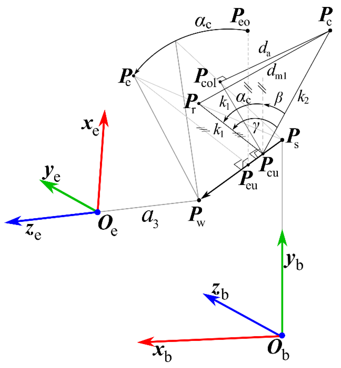
4.3. Computing the Minimum Distance and Respective Collision-Avoidance Angle α

Concerning Figure 3, let us consider a point, Pc, belonging to an obstacle located inside the space region where the robot moves and placed on one side of plane-π2, which is identified by the sign g . Additionally, let us consider the Pc projection points Pc1 and Pc2 onto the lines defined by the referential links PsPe and PePw, respectively [47]. The following relationships hold:
P c 1 = P s + P c P s P e P s P e P s P e P s 2 P c 2 = P e + P c P e P w P e P w P e P w P e 2
In the proposed algorithm, evaluating whether point Pc1 (Pc2) is inside the segment PsPe (segment PePw) is the first step. Both, just one, or even none of the two points may belong to their respective segments. Such an evaluation will be true if it is true that for the two parameters u1 and u2, defined as follows:
u 1 = P c 1 P s P e P s P c 1 P s P c 1 P s P e P s P e P s       u 2 = P c 2 P e P w P e P c 2 P e P c 2 P e P w P e P w P e ,
where the conditions u 1 0 , 1 and u 2 0 , 1 hold.
If Pc1 (Pc2) belongs to PsPe (to PePw), the next step consists of the computation of the three distances: d a = P c P c 1 if u 1 0 , 1 , d b = P c P e and d c = P c P c 2 if u 2 0 , 1 , which are the distances of Pc, respectively, from the referential link PsPe, the relevant point Pe, and the referential link PePw. Considering the minimum and maximum radii of the truncated cones (see Figure 2), the minimum allowed safety distance dm1 and dm2, for each cone of each link are calculated as follows:
d m 1 = 1 u 1 d cmin + u 1 d cmax d m 2 = 1 u 2 d cmax + u 2 d cmin
The collision will be imminent if da < dm1 or db < dcmax or dc < dm2. The three inequalities can be false, which implies that there is no possibility of collision; that is, αc(n) = 0 rad (see Equations (2) and (3)). Differently, if one or more inequalities are true, one or more points on the robot’s kinematic chain are under collision imminence. In this case, with only one degree of redundancy and, therefore, only one possible additional movement, the smallest among the minimum distances exceeded (da or db or dc) will be identified and will serve as a reference for calculating angle αc(n) (see Figure 4).
Let us consider the case (see Figure 4) where the minimum distance between the point Pc and the robot link PsPe is less than the allowed distance dm1. Angle αc(n) must make the distance between Pc and its projection, Pcol, onto PsPe at least equal to dm1, which implies moving Pcol from its initial position to at least point Pr of Figure 4 by changing α (see Figure 1b).
Let Pcu be the projection point of Pc onto the line segment PsPw, calculated as follows:
P cu = P s + P c P s P w P s P w P s P w P s 2
Thus, inspecting Figure 4, one notes that the angle αc(n) = γ β , with
γ = Atan 2 sign ( g ) 1 k 1 2 + k 2 2 d m 1 2 2 k 1 k 2 2 , k 1 2 + k 2 2 d m 1 2 2 k 1 k 2 β = Atan 2 sign ( g ) 1 v 1 v 2 2 , v 1 v 2
where k 1 = P col P cu , and k 2 = P c P cu , v 1 = P eo P eu P eo P eu , v 2 = P c P eu P c P eu , and g = P c P cu × P col P cu P w P s . The sign of g indicates which side of plane-π2 point Pc belongs to (see Figure 3) and determines the rotation direction of the angles γ and β.
For the nth iteration of the trajectory generation, the previous steps can be summarized in Algorithm 1.
Algorithm 1. Computation of angle α f at the nth iteration.
1Input
2Desired position and orientation of the end-effector at the iteration n;
3Compute the inverse kinematics for αc = 0 rad;
4Coordinates of the points belonging to the referential links and relevant points           % In this development Ps, Pe and Pw
5 Retrieve   the   values   of   α c ( n 1 ) , α c ( n 2 ) , α f ( n 1 ) , α f ( n 2 )
6Pc % Coordinates of a possible collision point
7find← false; % Boolean variable to indicate if a collision point exists inside safety volume.
8dmc← 0; % Initializing the minimum of the minimal distances.
9Pcol← []; % Point in the kinematic chain with the minor distance to Pc.
10Compute u1 and u2;
11if  u 1 0 , 1  then % Pc1 is between Ps and Pe
12 d a = P c P c 1 ;
13 d m 1 = 1 u 1 d cmin + u 1 d cmax ;
14if da < dm1 then
15   dmcdm1; % saving the minimal allowed distance
16   PcolPc1; % saving the point on the kinematic chain
17   find← true;
end
18elseif u 2 0 , 1  then % Pc2 is between Pe and Pw
19 d c = P c P c 2 ;
20 d m 2 = 1 u 2 d cmin + u 2 d cmax ;
21if dc < dm2 then
22    if dc < da then
23     dmcdm2; % saving the minimal distance
24     PcolPc2; % saving the point on the kinematic chain
25     find← true;
    end if
end if
end if
26 d b = P c P e ; % evaluating the collision distance from Pcto the point Pe
27ifdb<dcmaxthen   % considering a sphere as safety region around Pesee Figure 2
28if find=false then;
29    dmcdb;
30    PcolPe;
31    find← true;
32elseif db<dmc then
33    dmcdb;
34    PcolPe;
end if
end if
35if find=false % if there is no need to avoid collision
36   α c ( n ) = 0 rad;
37   dmc=0;
else % computing the value of α c to move the robot away from the collision point.
38   Compute γ and β;
39 α c ( n ) = γ β ;
end if
40 α f ( n ) = h 1 α c ( n 1 ) + h 2 α c ( n 2 ) + b 1 α f ( n 1 ) + b 2 α f ( n 2 ) ; % Equation (3)
41Solve inverse kinematics using α f ( n ) ;
42Output Save joint positions;

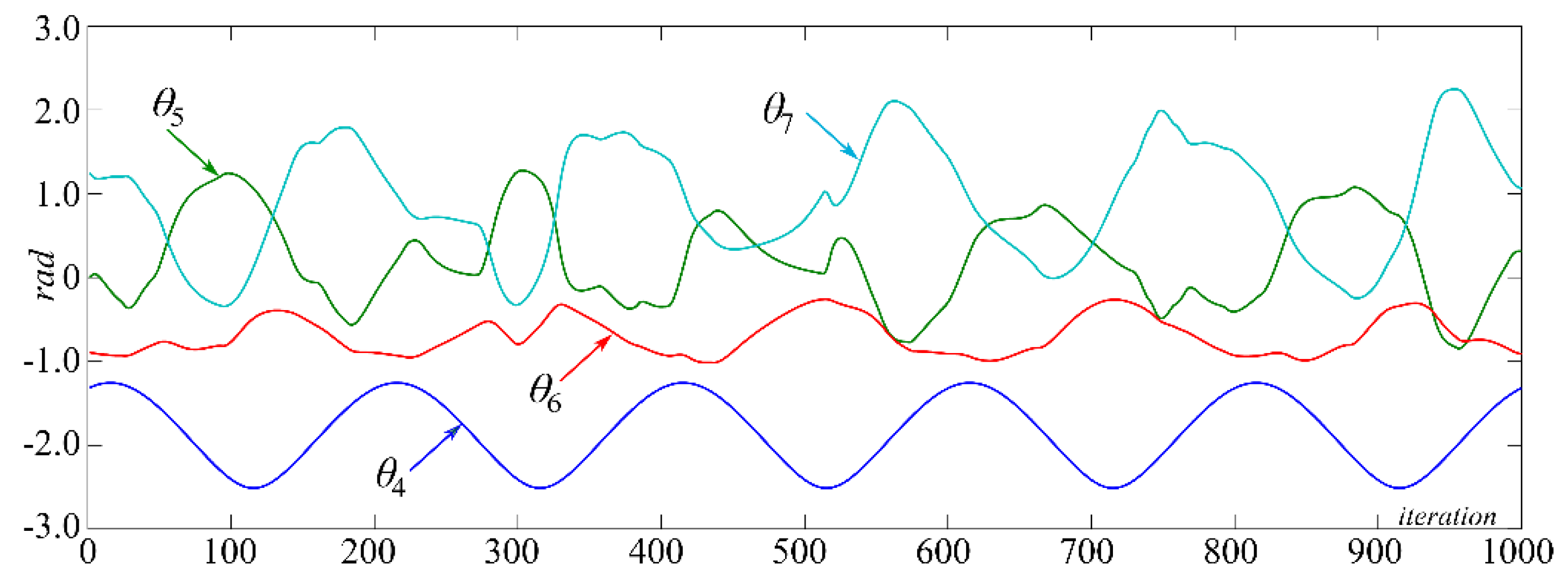
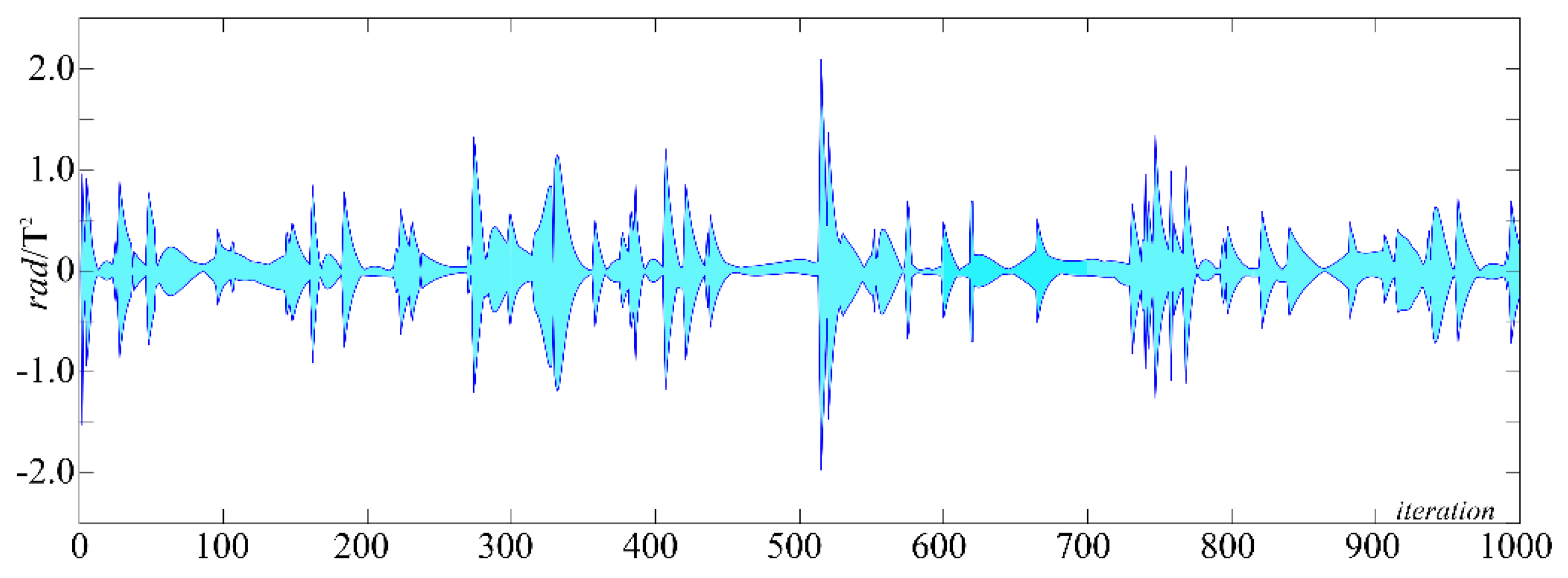
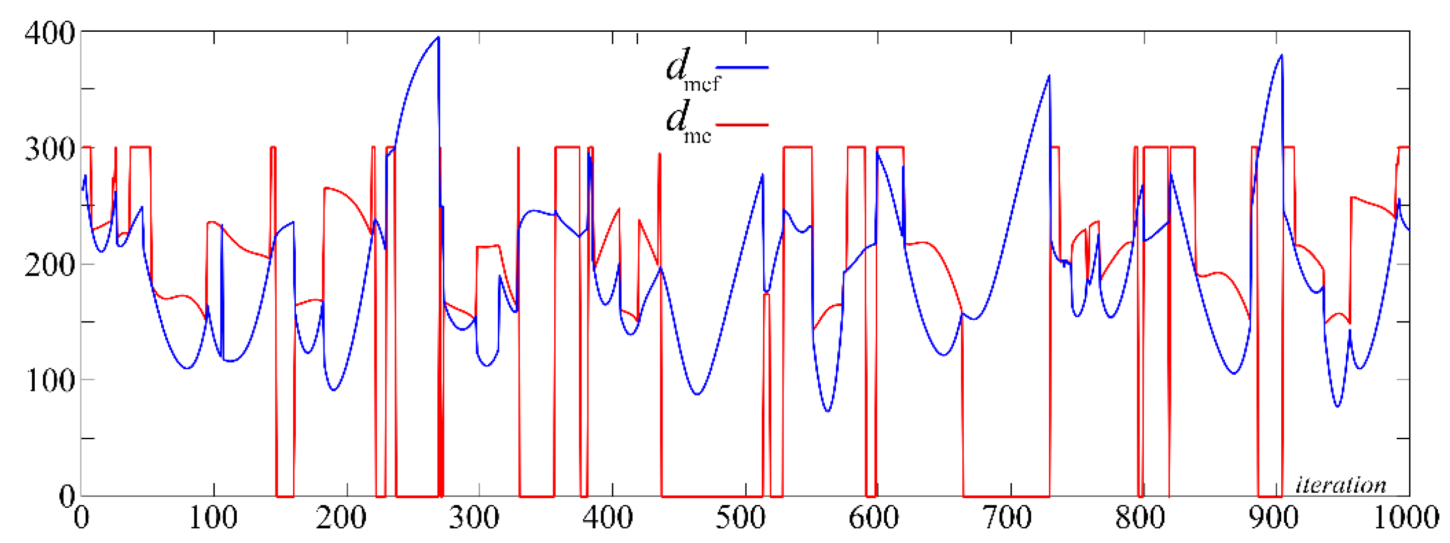
5. Graphical Results

Numerical simulations were conducted to validate the proposed collision-avoidance strategy. In these simulations, the Kuka-LBR-iiwa real lengths [45], that is, a0 = 340 mm, a1 = 400 mm, a2 = 400 mm, and a3 = 126 mm, were selected for the geometric model of the SRS-type robot. Additionally, the chosen motion task for the robot is an end-effector path (see Figure 2 and Figure 5) that keeps the ze axis perpendicular to the xbzb coordinate-plane and makes point Oe perform five rides along the circular trajectory, with the center at point [400 200 200]T mm and radius 200 mm, that lies on the plane yb = 200 mm. The robot motion is sampled in 1000 equidistant time-instants, and at every sampling instant, Algorithm 1 is executed.
The simulation environment, over the robot, includes two human arms identified as Human-arm 1 and Human-arm 2, composed of two links and located in the space by three points named shoulder, elbow, and hand, thus improving the experiments presented in [48], where only one arm is used. The links shoulder–elbow and elbow–hand have lengths [49] of 319.6 mm and 246.5 mm with angle displacement defined with respect to the xb-axis. The chosen motion for these two arms makes the three above-mentioned points perform oscillatory movements with the motion parameters reported in Table 1. Human-arm motion takes place while the robot’s end-effector performs the above-defined five circular paths with the center at [400 200 200]T mm and a radius of 200 mm.
The tests were developed on a laptop with an Intel Core i7 CPU (2.7 GHz, 8,00 Gb RAM), spending 3.68 s in execution. All the simulations were developed by using MATLAB R2021a. Eventually, the second-order transfer function, the reference for programming the filter, was adjusted with p = 0.2 s−1, and the sampling time was adjusted to T = 0.06 s, which corresponds to m = pT = 0.012 and a simulation cycle of 60 s. It is worth stressing that, to avoid muscular injuries, a worker should not execute motion cycles with a period lower than 60 s; so, in these simulations, the human-arm motion is much faster than the admitted one (i.e., the chosen parameters make the simulation environment much faster than a realistic one).
The graphical simulation environment presented in Figure 5 enables us to observe the evolution of the proposed algorithm and the SRS-type’s end-effector performance following the desired trajectory while dealing with collision avoidance.
A video that presents the complete simulation experiment of the proposed algorithm is available at [50] and as “Supplementary Materials” accompanying this paper. Figure 6 presents three frames from the above-mentioned video showing the SRS-type robot while avoiding a collision. The video shows that, in this simulation environment, a sampling rate (=1/T) of 16.7 Hz is sufficient to avoid collision with the proposed strategy. It is worth stressing that since this sampling rate corresponds to a “reaction time” of 60 ms for the robot and the human reaction time is about 200 ms, the proposed strategy can enable the robot to react three times faster than a human being.
Figure 7 shows the computed angle αc and its filtered counterpart αf, used as a reference for the inverse kinematics, during the simulation cycle. The analysis of Figure 7 reveals that αf is a regular curve.
Figure 8 and Figure 9 show the rates of angle and angular speed as a function of the sampling period T to evaluate the continuity and smoothness of the trajectory for the filtered angle αf.
The inverse-kinematics solution of the SRS-type robot yields the position profile of joints 1, 2, and 3, which are θ1, θ2, and θ3, respectively, presented in Figure 10; as well as joints 4, 5, 6, and 7, which are θ4, θ5, θ6, and θ7, respectively, presented in Figure 11.
For each iteration, and considering the known sampling time T, the rates of changes of joint variables and corresponding accelerations were calculated for each joint by first-order approximations. Thus, taking the maximum and minimum values obtained, Figure 12 and Figure 13 show the range achieved for the rate of change of position and acceleration, respectively, in each iteration of all robot joint variables. The rates of joint positions and acceleration behavior did not show abrupt variations, remaining in a limited range with similar magnitudes.
The angle αf smooths the resultant distances between the robot and the collision point. Figure 14 shows the behavior of the distance between the SRS-type robot and the collision point (red) along the simulation, compared with the distances when under imminent collision (blue). It is worth mentioning that when the robot is out of collision avoidance, the distance dmc used to calculate the angle αf is adjusted to 0, as seen in line 37 of Algorithm 1.

6. Discussions

The results presented in the test showed that the proposed algorithm smoothed all the joints’ position and velocity profiles in a dynamic environment.
The test aims at replicating the relationship between a collision point crossing a circle and the consequent problem of variation in the resulting distances projected on the robot’s links. Although the collision curve is deterministic in the test, the procedure applies to random variations in the collision point coordinates or a more significant number of collision points, including the number of links and relevant robot points. The algorithm can deal with multiple collision points, attempting to move the robot away from that nearest collision point. For the collision avoidance on k simultaneous collision points, the robot should have a redundancy index r = k; for example, if it is necessary to have three collision points or control the three distances, such as da, db, and dc discussed in Section 4.3, the robot should have degrees of redundancy r = 3. In this way, the algorithm should be executed three times for each collision point featuring its expandability.
The presented inverse kinematics, which solves the α angle for the four quadrants, is based on review propositions [8,39,48] and refines them, thus improving the formulation.
Additionally, in the presented simulation, the available degree of redundancy is 1, and it is strictly sufficient to solve the collision-avoidance problem without including the joint limits control, as was achieved in other papers [15,20,48,51,52,53] where the introduced redundancy was exploited by optimization procedures to find the best α that avoids reaching joint-position limits. The possible involvement of joint-position limits’ control, over collision avoidance, in programming trajectories and kinematic algorithms solely depends on the availability of redundancy degrees higher than one, which, if available, can be exploited by implementing one of the strategies proposed in the literature, even with the proposed algorithm.
Similar algorithms present safety volumes described by a limited number of points [44,54] or based on numerical approaches [4,20]. The here-discussed proposal uses a parametric surface around the links, instead of limited volumes as discussed in [4], to define the safety volume in the computation of the collision distance for any point of the link, which makes this new approach more realistic and reliable.
At the same time, the use of a second-order filter makes the strategy feasible, adjustable, and replicable, ensuring, together with the description of the safety volume, smooth transients in the trajectories as well as an analytical collision-avoidance algorithm without numerical procedures that increase the computational burden, as found in [23]. The smoothing of the collision-avoidance transients appears in the bounded rate of positions and acceleration profiles for the robot joints (see Figure 12 and Figure 13), continuously ensuring that discontinuities, such as those shown in [4,54,55], do not arise despite the dynamic environment.
Using a digital filter in the transition between paths to be followed by the joints additionally guarantees the smoothness of the programmed trajectories.
It is important to note that the collision-avoidance algorithm’s proposition has limitations when several collision points or several links lead to opposite displacements generating conflicts of movements characterizing singularities. Concerning the singularities, it is observed that collision avoidance does not occur when g = 0, or the collision point Pc belongs to the plane formed by the points Ps, Pw, and Pe, as can be seen in Figure 3 and Figure 4; that is,
D = P c P s n p n p = 0
where D corresponds to the distance between the point Pc and the plane formed by the points Ps, Pw, and Pe, and np is the result of a cross-product as follows:
n p = P e P s P e P s × P w P e P w P e
It is interesting to note that angle α f does not produce errors of position and orientation of the end effector, despite the need for a time of accommodation or convergence to the final values following trajectories, since its primary task is to control the distance from the collision.
However, the need for transitory times for collision avoidance means suitable adjustments to the filter time constant according to the desired performance and control specifications.
The proposed algorithm can deal with collision avoidance between multiple robots simultaneously. In this case, the distance between the robot’s links is controlled by calculating the geometric distance between the line segments to which the links belong. Thus, taking a robot as a reference, the Pc points belong to the other robots, and running the proposed algorithm in each robot’s trajectory generator allows several robots to share the same space without generating collisions.

7. Conclusions

Workspaces shared between robots and humans in collaborative tasks require strategies that include collision avoidance and the programming of smooth transitional displacements.
This paper presented an algorithm for the treatment of collision and posture adjustment of robots based on analytical spatial geometry and the use of digital second-order critically damped filters. The strategy includes a posture adjustment of the robot based on an additional movement, defined as α, available for the redundant 7-DOF SRS-type robot. The simulations showed the smoothing of the joints’ trajectory profiles and collision avoidance effectiveness without collisions in a dynamic environment.
The geometric approach allowed us to present a proposition for inverse kinematics considering the posture adjustment and the projection of the collision point on any point on the links of the robot’s kinematic chain.
Spatial surfaces were used as an example for the determination of the safety regions of the robot. For relevant points and links (under imminent collision), we used the formulation of spheres and truncated cones, which allows us to identify the possibility of collision and activate the collision-avoidance strategy. According to the geometry of links and components that form the environment where the robot is inserted, other formulations can be adapted and used as safety surfaces.
The proposed collision-avoidance solution is feasible and straightforward, providing a quick implementation solution for collaborative robots. The fact that the proposal is based only on analytical formulations reduces the computational effort, thus increasing the reliability of the solutions for trajectories and the efficiency of collision control and other processing in each sampling time.

Supplementary Materials

The following supporting information can be downloaded at: https://www.mdpi.com/article/10.3390/robotics11050093/s1.

Author Contributions

Conceptualization, H.S. and R.D.G.; Funding acquisition, R.D.G.; Methodology, H.S. and R.D.G.; Software, H.S.; Supervision, R.D.G.; Validation, H.S.; Writing–original draft, H.S.; Writing–review & editing, R.D.G. All authors have read and agreed to the published version of the manuscript.

Funding

This research was developed at the Laboratory of Mechatronics and Virtual Prototyping (LaMaViP) of Ferrara Technopole, supported by the UNIFE FAR2020 fund, in partnership with the Raul Guenther Laboratory of Applied Robotics of the Federal University of Santa Catarina, supported by CNPq–Conselho Nacional de Desenvolvimento Científico e Tecnológico (National Council for Scientific and Technological Development) project 307249/2021-2, Brazil.

Institutional Review Board Statement

Not applicable.

Informed Consent Statement

Not applicable.

Data Availability Statement

This work does not use experimental data. The data necessary to replicate the computations illustrated in the paper are included in the text of the paper.

Conflicts of Interest

The authors declare no conflict of interest.

References

  1. Mihelj, M.; Bajd, T.; Ude, A.; Lenarcic, J.; Stanovnik, A.; Munih, M.; Rejc, J.; Šlajpah, S. Robotics, 2nd ed.; Springer: Cham, Switzerland, 2018. [Google Scholar] [CrossRef]
  2. Matheson, E.; Minto, R.; Zampieri, E.G.G.; Faccio, M.; Rosati, G. Human–Robot Collaboration in Manufacturing Applications: A Review. Robotics 2019, 8, 100. [Google Scholar] [CrossRef]
  3. El Zaatari, S.; Marei, M.; Li, W.; Usman, Z. Cobot Programming for Collaborative Industrial Tasks: An Overview. Robot. Auton. Syst. 2019, 116, 162–180. [Google Scholar] [CrossRef]
  4. Safeea, M.; Neto, P.; Bearee, R. On-Line Collision Avoidance for Collaborative Robot Manipulators by Adjusting off-Line Generated Paths: An Industrial Use Case. Robot. Auton. Syst. 2019, 119, 278–288. [Google Scholar] [CrossRef]
  5. Alebooyeh, M.; Urbanic, R.J. Neural Network Model for Identifying Workspace, Forward and Inverse Kinematics of the 7-DOF YuMi 14000 ABB Collaborative Robot. IFAC-PapersOnLine 2019, 52, 176–181. [Google Scholar] [CrossRef]
  6. IFR. A Positioning Paper: Demystifying Collaborative Industrial Robots; International Federation of Robotics: Frankfurt, Germany, 2018; pp. 1–5. [Google Scholar]
  7. ISO/TS 15066:2016; Robots and Robotic Devices—Collaborative Robots. ISO: Geneva, Switzerland, 2016.
  8. Busson, D.; Bearee, R.; Olabi, A. Task-Oriented Rigidity Optimization for 7 DOF Redundant Manipulators. IFAC-PapersOnLine 2017, 50, 14588–14593. [Google Scholar] [CrossRef]
  9. Liu, W.; Chen, D.; Steil, J. Analytical Inverse Kinematics Solver for Anthropomorphic 7-DOF Redundant Manipulators with Human-Like Configuration Constraints. J. Intell. Robot. Syst. Theory Appl. 2017, 86, 63–79. [Google Scholar] [CrossRef]
  10. Zhang, L.; Xiao, N. A Novel Artificial Bee Colony Algorithm for Inverse Kinematics Calculation of 7-DOF Serial Manipulators. Soft Comput. 2019, 23, 3269–3277. [Google Scholar] [CrossRef]
  11. Liu, M.C.; Tsai, H.H.; Hsiao, T. Kinematics-Based Studies on a 7-DOF Redundant Manipulator. In Proceedings of the 2014 CACS International Automatic Control Conference (CACS 2014), Kaohsiung, Taiwan, 26–28 November 2014; pp. 228–231. [Google Scholar] [CrossRef]
  12. Di Gregorio, R.; Simas, H. Dimensional Synthesis of the Single-Loop Translational Parallel Manipulator PRRR-PRPU. Meccanica 2018, 53, 481–495. [Google Scholar] [CrossRef]
  13. Simas, H.; Martins, D.; Di Gregorio, R. Smooth Path Planning for Redundant Robots on Collision Avoidance. In Mechanisms and Machine Science; Springer: Cham, Switzerland, 2019; Volume 73, pp. 1869–1878. [Google Scholar] [CrossRef]
  14. Simas, H.; Guenther, R.; Da Cruz, D.F.M.; Martins, D. A New Method to Solve Robot Inverse Kinematics Using Assur Virtual Chains. Robotica 2009, 27, 1017–1026. [Google Scholar] [CrossRef]
  15. Rouhani, M.; Ebrahimabadi, S. Inverse Kinematics of a 7-DOF Redundant Robot Manipulator Using the Active Set Approach under Joint Physical Limits. Turk. J. Electr. Eng. Comput. Sci. 2017, 25, 3920–3931. [Google Scholar] [CrossRef]
  16. Osa, T. Multimodal Trajectory Optimization for Motion Planning. Int. J. Robot. Res. 2020, 39, 983–1001. [Google Scholar] [CrossRef]
  17. Dereli, S.; Köker, R. Calculation of the Inverse Kinematics Solution of the 7-DOF Redundant Robot Manipulator by the Firefly Algorithm and Statistical Analysis of the Results in Terms of Speed and Accuracy. Inverse Probl. Sci. Eng. 2020, 28, 601–613. [Google Scholar] [CrossRef]
  18. Ayten, K.K.; Sahinkaya, M.N.; Dumlu, A. Real Time Optimum Trajectory Generation for Redundant/Hyper-Redundant Serial Industrial Manipulators. Int. J. Adv. Robot. Syst. 2017, 14, 172988141773724. [Google Scholar] [CrossRef]
  19. Siciliano, B. Kinematic Control of Redundant Robot Manipulators: A Tutorial. J. Intell. Robot. Syst. 1990, 3, 201–212. [Google Scholar] [CrossRef]
  20. Quispe, A.H.; Stilman, M. Deterministic Motion Planning for Redundant Robots along End-Effector Paths. In Proceedings of the 2012 12th IEEE-RAS International Conference on Humanoid Robots (Humanoids 2012), Osaka, Japan, 29 November–1 December 2012; pp. 785–790. [Google Scholar] [CrossRef]
  21. Zanchettin, A.M.; Rocco, P. A General User-Oriented Framework for Holonomic Redundancy Resolution in Robotic Manipulators Using Task Augmentation. IEEE Trans. Robot. 2012, 28, 514–521. [Google Scholar] [CrossRef]
  22. Klein, C.A.; Huang, C.H. Review of Pseudoinverse Control for Use with Kinematically Redundant Manipulators. IEEE Trans. Syst. Man Cybern. 1983, SMC-13, 245–250. [Google Scholar] [CrossRef]
  23. Kalakrishnan, M.; Chitta, S.; Theodorou, E.; Pastor, P.; Schaal, S. STOMP: Stochastic Trajectory Optimization for Motion Planning. In Proceedings of the 2011 IEEE International Conference on Robotics and Automation, Shanghai, China, 9–13 May 2011; pp. 4569–4574. [Google Scholar] [CrossRef]
  24. Besset, P.; Béarée, R. FIR Filter-Based Online Jerk-Constrained Trajectory Generation. Control Eng. Pract. 2017, 66, 168–180. [Google Scholar] [CrossRef]
  25. Gerelli, O.; Guarino Lo Bianco, C. A Discrete-Time Filter for the on-Line Generation of Trajectories with Bounded Velocity, Acceleration, and Jerk. In Proceedings of the 2010 IEEE International Conference on Robotics and Automation, Anchorage, AK, USA, 3–7 May 2010; pp. 3989–3994. [Google Scholar] [CrossRef]
  26. Biagiotti, L.; Melchiorri, C. Online Trajectory Planning and Filtering for Robotic Applications via B-Spline Smoothing Filters. In Proceedings of the 2013 IEEE/RSJ International Conference on Intelligent Robots and Systems, Tokyo, Japan, 3–7 November 2013; pp. 5668–5673. [Google Scholar] [CrossRef]
  27. Preiss, J.A.; Hausman, K.; Sukhatme, G.S.; Weiss, S. Simultaneous Self-Calibration and Navigation Using Trajectory Optimization. Int. J. Robot. Res. 2018, 37, 1573–1594. [Google Scholar] [CrossRef]
  28. Franklin, G.F.; Powell, J.D.; Emami-Naeini, A. Feedback Control of Dynamic Systems, 8th ed.; Pearson: London, UK, 2019. [Google Scholar]
  29. Colome, A.; Torras, C. Redundant Inverse Kinematics: Experimental Comparative Review and Two Enhancements. In Proceedings of the 2012 IEEE/RSJ International Conference on Intelligent Robots and Systems, Vilamoura-Algarve, Portugal, 7–12 October 2012; pp. 5333–5340. [Google Scholar] [CrossRef]
  30. Siciliano, B.; Lorenzo, S.; Villani, L.; Orilo, G. Robotics: Modelling, Planning and Control, 2nd ed.; Springer: London, UK, 2010. [Google Scholar]
  31. Tsai, L.-W. Robot Analysis and Design: The Mechanics of Serial and Parallel Manipulators, 1st ed.; John Wiley & Sons, Inc.: Hoboken, NJ, USA, 1999. [Google Scholar]
  32. Dereli, S.; Köker, R. A Meta-Heuristic Proposal for Inverse Kinematics Solution of 7-DOF Serial Robotic Manipulator: Quantum Behaved Particle Swarm Algorithm. Artif. Intell. Rev. 2020, 53, 949–964. [Google Scholar] [CrossRef]
  33. Mooney, J.G.; Johnson, E.N. A Comparison of Automatic Nap-of-the-Earth Guidance Strategies for Helicopters. J. Field Robot. 2014, 33, 1–17. [Google Scholar] [CrossRef]
  34. Zhao, S.; Zhu, Z.; Luo, J. Multitask-Based Trajectory Planning for Redundant Space Robotics Using Improved Genetic Algorithm. Appl. Sci. 2019, 9, 2226. [Google Scholar] [CrossRef]
  35. Ogura, Y.; Aikawa, H.; Shimomura, K.; Kondo, H.; Morishima, A.; Lim, H.O.; Takanishi, A. Development of a New Humanoid Robot WABIAN-2. In Proceedings of the 2006 IEEE International Conference on Robotics and Automation, 2006. ICRA 2006, Orlando, FL, USA, 15–19 May 2006; pp. 76–81. [Google Scholar] [CrossRef]
  36. Starke, S.; Hendrich, N.; Krupke, D.; Zhang, J. Evolutionary Multi-Objective Inverse Kinematics on Highly Articulated and Humanoid Robots. In Proceedings of the 2017 IEEE/RSJ International Conference on Intelligent Robots and Systems (IROS), Vancouver, BC, Canada, 24–28 September 2017; pp. 6959–6966. [Google Scholar] [CrossRef]
  37. Lim, J.; Oh, J.-H. Backward Ladder Climbing Locomotion of Humanoid Robot with Gain Overriding Method on Position Control. J. Field Robot. 2016, 33, 687–705. [Google Scholar] [CrossRef]
  38. Faria, C.; Ferreira, F.; Erlhagen, W.; Monteiro, S.; Bicho, E. Position-Based Kinematics for 7-DoF Serial Manipulators with Global Configuration Control, Joint Limit and Singularity Avoidance. Mech. Mach. Theory 2018, 121, 317–334. [Google Scholar] [CrossRef]
  39. Wang, Y.; Artemiadis, P. Closed-Form Inverse Kinematic Solution for Anthropomorphic Motion in Redundant Robot Arms. Adv. Robot. Autom. 2013, 2(3), 1000110. [Google Scholar] [CrossRef]
  40. Simas, H.; Di Gregorio, R. Position Analysis, Singularity Loci and Workspace of a Novel 2PRPU Schoenflies-Motion Generator. Robotica 2019, 37, 141–160. [Google Scholar] [CrossRef]
  41. Simas, H.; Di Gregorio, R. Kinetostatics and Optimal Design of a 2PRPU Shoenflies-Motion Generator. In Mechanisms and Machine Science; Springer Cham: Cham, Switzerland, 2017; Volume 54. [Google Scholar] [CrossRef]
  42. Mohammed, A.; Schmidt, B.; Wang, L. Active Collision Avoidance for Human–Robot Collaboration Driven by Vision Sensors. Int. J. Comput. Integr. Manuf. 2017, 30, 970–980. [Google Scholar] [CrossRef]
  43. Süli, E.; Mayers, D.F. An Introduction to Numerical Analysis; Cambridge University Press: New York, NY, USA, 2003. [Google Scholar] [CrossRef]
  44. Luo, R.C.; Ko, M.C.; Chung, Y.T.; Chatila, R. Repulsive Reaction Vector Generator for Whole-Arm Collision Avoidance of 7-DoF Redundant Robot Manipulator. In Proceedings of the 2014 IEEE/ASME International Conference on Advanced Intelligent Mechatronics, Besacon, France, 8–11 July 2014; pp. 1036–1041. [Google Scholar] [CrossRef]
  45. KUKA Sensitive Robotics: LBR iiwa. Catalog published by KUKA Roboter GmbH: Augsburg, Germany. 2016. Available online: https://pdf.directindustry.com/pdf/kuka-ag/kuka-sensitive-robotics-lbr-iiwa/17587-724449.html (accessed on 9 July 2022).
  46. Huber, G.; Wollherr, D. Efficient Closed-Form Task Space Manipulability for a 7-DOF Serial Robot. Robotics 2019, 8, 98. [Google Scholar] [CrossRef] [Green Version]
  47. Larson, R.; Edwards, B.H. Multivariable Calculus, 9th ed.; Cengage Learning: Boston, MA, USA, 2009. [Google Scholar]
  48. Herrera Pineda, J.C.; Mejia Rincon, L.; Simoni, R.; Simas, H. Maximum Isotropic Force Capability Maps in Planar Cooperative Systems: A Practical Case Study. In Mechanisms and Machine Science; Springer: Cham, Switzerland, 2018; Volume 54, pp. 160–170. [Google Scholar] [CrossRef]
  49. Oh, J.; Bae, H.; Oh, J.H. Analytic Inverse Kinematics Considering the Joint Constraints and Self-Collision for Redundant 7DOF Manipulator. In Proceedings of the 2017 First IEEE International Conference on Robotic Computing (IRC), Taichung, Taiwan, 10–12 April 2017; pp. 123–128. [Google Scholar] [CrossRef]
  50. Video that presents the complete simulation experiment. Available online: https://youtu.be/BfRjA8dgnq8 (accessed on 9 July 2022).
  51. Frantz, J.C.; Rincon, L.M.; Simas, H.; Martins, D. Wrench Distribution of a Cooperative Robotic System Using a Modified Scaling Factor Method. J. Braz. Soc. Mech. Sci. Eng. 2018, 40, 177. [Google Scholar] [CrossRef]
  52. Zhou, D.; Ji, L.; Zhang, Q.; Wei, X. Practical Analytical Inverse Kinematic Approach for 7-DOF Space Manipulators with Joint and Attitude Limits. Intell. Serv. Robot. 2015, 8, 215–224. [Google Scholar] [CrossRef]
  53. Scimmi, L.S.; Melchiorre, M.; Mauro, S.; Pastorelli, S. Multiple Collision Avoidance between Human Limbs and Robot Links Algorithm in Collaborative Tasks. In Proceedings of the 15th International Conference on Informatics in Control, Automation and Robotics, Porto, Portugal, 29–31 July 2018; pp. 291–298. [Google Scholar] [CrossRef]
  54. Karimi, G.; Jahanian, O. Genetic Algorithm Application in Swing Phase Optimization of AK Prosthesis with Passive Dynamics and Biomechanics Considerations. In Genetic. Algorithms Application; Intechopen: London, UK, 2012; pp. 71–88. [Google Scholar] [CrossRef]
  55. Xu, Z.; Gan, Y.; Dai, X. Obstacle Avoidance of 7-DOF Redundant Manipulators. In Proceedings of the 2019 Chinese Control And Decision Conference (CCDC), Nanchang, China, 3–5 June 2019; pp. 4184–4189. [Google Scholar] [CrossRef]
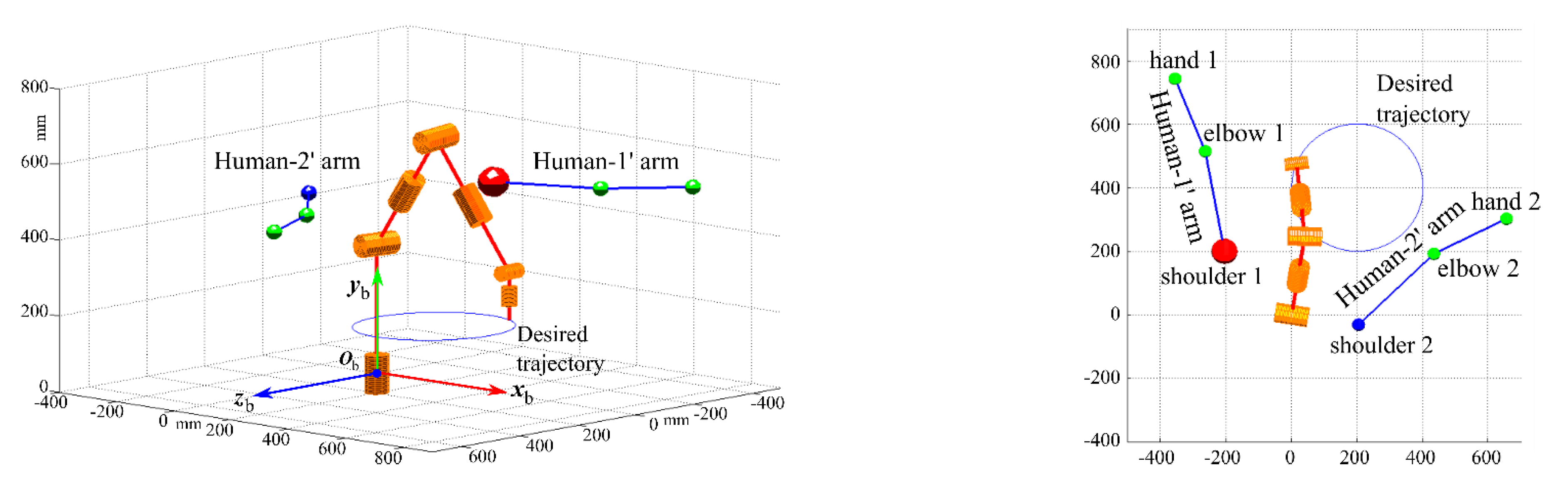
Figure 1. 7-DOF SRS-type redundant robot: (a) joint-variables’ phase-references; (b) geometrical parameters.
Robotics 11 00093 g001
Figure 2. SRS-type robot with its safety volume.
Robotics 11 00093 g002
Figure 3. Obstacle point Pc on left or right of plane-π2 and its projection points Pc1 and Pc2.
Robotics 11 00093 g003
Figure 4. Case with the collision point, Pcol, belonging to the segment PsPe: computation of the αc value for avoiding collision.
Robotics 11 00093 g004
Figure 5. Virtual simulation environment at iteration 390. Blue ball—shoulder coordinates; green ball—coordinates of the elbows and hands; red ball—point under imminent collision.
Robotics 11 00093 g005
Figure 6. Frames from the simulation video at iteration (a) 76; (b) 179; (c) 407.
Robotics 11 00093 g006
Figure 7. Comparison between the computed angle αc and its filtered αf used to solve the inverse kinematics.
Robotics 11 00093 g007
Figure 8. Computed rate of change of αf.
Robotics 11 00093 g008
Figure 9. Computed rate of change of α ˙ f .
Robotics 11 00093 g009
Figure 10. Result of the inverse kinematic for SRS-type robot joints 1, 2, and 3.
Robotics 11 00093 g010
Figure 11. Result of the inverse kinematic for SRS-type robot joints 4, 5, 6, and 7.
Robotics 11 00093 g011
Figure 12. Range of computed maximum and minimum rates of change of joint variables.
Robotics 11 00093 g012
Figure 13. Range of computed maximum and minimum accelerations of joint.
Robotics 11 00093 g013
Figure 14. Computed dmc distances from obstacle and the SRS-type robot along the simulation and the respective distance dmcf used to compute the αf when under collision imminence.
Robotics 11 00093 g014
Table 1. Human-arms simulation parameters.
Human-Arm 1Human-Arm 2
Base (shoulder)[−50 500 250]T mm[150 500 −200]T mm
Base rotation radius (around y-axis)50 mm50 mm
Base number of turns511
Shoulder angle range0.4 rad0.4 rad
Shoulder angle offset0.4 rad0.2 rad
Shoulder number of turns913
Elbow angle range0.4 rad0.4 rad
Elbow angle offset0.4 rad0 rad
Elbow number of turns79
Publisher’s Note: MDPI stays neutral with regard to jurisdictional claims in published maps and institutional affiliations.

