Review

A Comprehensive Survey of Visual SLAM Algorithms

Laboratoire Capteurs et Architectures Électroniques (LCAE), Laboratoire d’Intégration des Systèmes et des Technologies (LIST), Commissariat à l’Énergie Atomique et aux Énergies Alternatives (CEA), 91400 Saclay, France
*
Author to whom correspondence should be addressed.
Robotics 2022, 11(1), 24; https://doi.org/10.3390/robotics11010024
Submission received: 12 December 2021 / Revised: 27 January 2022 / Accepted: 7 February 2022 / Published: 10 February 2022
(This article belongs to the Topic Motion Planning and Control for Robotics)

Abstract

:
Simultaneous localization and mapping (SLAM) techniques are widely researched, since they allow the simultaneous creation of a map and the sensors’ pose estimation in an unknown environment. Visual-based SLAM techniques play a significant role in this field, as they are based on a low-cost and small sensor system, which guarantees those advantages compared to other sensor-based SLAM techniques. The literature presents different approaches and methods to implement visual-based SLAM systems. Among this variety of publications, a beginner in this domain may find problems with identifying and analyzing the main algorithms and selecting the most appropriate one according to his or her project constraints. Therefore, we present the three main visual-based SLAM approaches (visual-only, visual-inertial, and RGB-D SLAM), providing a review of the main algorithms of each approach through diagrams and flowcharts, and highlighting the main advantages and disadvantages of each technique. Furthermore, we propose six criteria that ease the SLAM algorithm’s analysis and consider both the software and hardware levels. In addition, we present some major issues and future directions on visual-SLAM field, and provide a general overview of some of the existing benchmark datasets. This work aims to be the first step for those initiating a SLAM project to have a good perspective of SLAM techniques’ main elements and characteristics.

1. Introduction

Simultaneous localization and mapping (SLAM) technology, first proposed by Smith in 1986 [1], is used in an extensive range of applications, especially in the domain of augmented reality (AR) [2,3,4] and robotics [5,6,7]. The SLAM process aims at mapping an unknown environment and simultaneously locating a sensor system in this environment through the signals provided by the sensor(s). In robotics, the construction of a map is a crucial task, since it allows the visualization of landmarks, facilitating the environment’s visualization. In addition, it can help in the state estimation of the robot, relocating it, and decreasing estimation errors when re-visiting registered areas [8].
The map construction comes with two other tasks: localization and path planning. According to Stachniss [9], the mapping problem may be described by examining three questions considering the robot’s perspective: What does the world look like? Where am I? and How can I reach a given location? The first question is clarified by the mapping task, which searches to construct a map, i.e., a model of the environment. To do so, it requires the location of the observed landmarks, i.e., the answer for the second question, provided by the localization task. The localization task searches to determine the robot’s pose, i.e., its orientation and position and, consequently, locates the robot on the map. Depending on the first two tasks, the path planning clears up the last question, and seeks to estimate a trajectory for the robot to achieve a given location. It relies on the current robot’s pose, provided by the localization task, and on the environment’s characteristics, provided by the mapping task. SLAM is a solution that integrates both the mapping and localization tasks.
Visual-based SLAM algorithms can be considered especially attractive, due to their sensor configuration simplicity, miniaturized size, and low cost. Therefore, numerous visual-based techniques are proposed in the literature, which make the choice of the most suitable one according to one’s project constraints difficult. The visual-based approaches can be divided into three main categories: visual-only SLAM, visual-inertial (VI) SLAM, and RGB-D SLAM. The first one refers to the SLAM techniques based only on 2D images provided by a monocular or stereo camera. They present a higher technical difficulty due to their limited visual input [10]. The robustness in the sensor’s tracking of the visual-SLAM algorithms may be increased by adding an inertial measurement unit (IMU), which can be found in their miniaturized size and low cost, while achieving high accuracy, essential aspects to many applications that require lightweight design, such as autonomous race cars [11]. In addition, visual-based SLAM systems may employ a depth sensor and process the depth information by applying a RGB-D-based approach.
To obtain a general overview and an introduction to the SLAM problem, the work by Durrant-White and Bailey [12,13] proposes a SLAM tutorial presenting from the problem description to the environment representations. In addition, Cadena et al. [8] analyzes the main open problems and future perspectives of the SLAM. Considering the reviews and surveys of visual-based techniques, Yousif et al. [14] and Fuentes-Pacheco et al. [15] present an overview of the main concepts used in the visual-only SLAM techniques and the fundamental algorithms. Yousif et al. [14] also briefly describes the RGB-D-based SLAM problem. Taketomi et al. [10] and Covolan et al. [3] present an overview of the main concepts used in the visual-based SLAM approaches, focusing on visual-only and RGB-D-based approaches and describing the main algorithms. The recent publication by Servieres et al. [16] proposes a classification of the main visual-based SLAM algorithms and performs a historical research.
Gui et al. [17] and Chen et al. [18] present the main concepts and algorithms of visual-inertial SLAM and visual-inertial odometry approaches, considering the filtering-based and optimization-based perspectives. In [17], the techniques up to 2015 are presented, while in [18], the algorithms up to 2018 are also included. An overview of the main concepts and techniques in visual-inertial navigation can also be found in [19]. Concerning the RGB-D approaches, Chen et al. [20] presents a global perspective from the main concepts used in RGB-D modeling. A recent survey by Zhang et al. [21] presents an overview of the main concepts and describes the principal RGB-D-based SLAM algorithms. As one can see, there are several reviews and surveys in the literature about visual-based SLAM techniques; still, most of them are limited to just one or two of the three main approaches and do not address the algorithms in detail. So, a review that addresses the three approaches and the fundamental algorithms is necessary to help researchers and students to initiate their works on visual-SLAM techniques to obtain an overview of this large domain.
Thus, this paper provides a review of the most representative visual-based SLAM techniques and an overview of each method’s main advantages and disadvantages. This article presents three main contributions: 1—An explanation of the most representative visual-based SLAM algorithms through the construction of diagrams and flowcharts. This approach will be helpful to the reader, as it provides an overview of the SLAM techniques when initiating a project and allows the reader to have a first contact with the visual-based SLAM algorithms. 2—As far as we know, this is the first review article that presents the three main visual-based approaches, performing an individual analysis of each method and a general analysis of the approaches. 3—Focusing on the readers initiating their studies on the SLAM algorithms, we propose six main criteria to be observed in the different techniques and implementations to be considered according to one’s application. The requirements consider, from a software level, SLAM techniques, such as loop closure, to a hardware-level approach, such as SLAM on SoC implementations.
This paper is organized as follows. Section 2 presents the main essential concepts of the three selected approaches. Section 3 presents the six criteria that we established to evaluate the SLAM algorithms and the most representative SLAM techniques according to the presented approaches. Section 4 presents some of the recent major issues faced by the visual-SLAM community and points out future directions to deal with these problems. Section 5 provides a general overview of some of the most significant publicly available benchmark datasets. Finally, our conclusions are presented in Section 6.

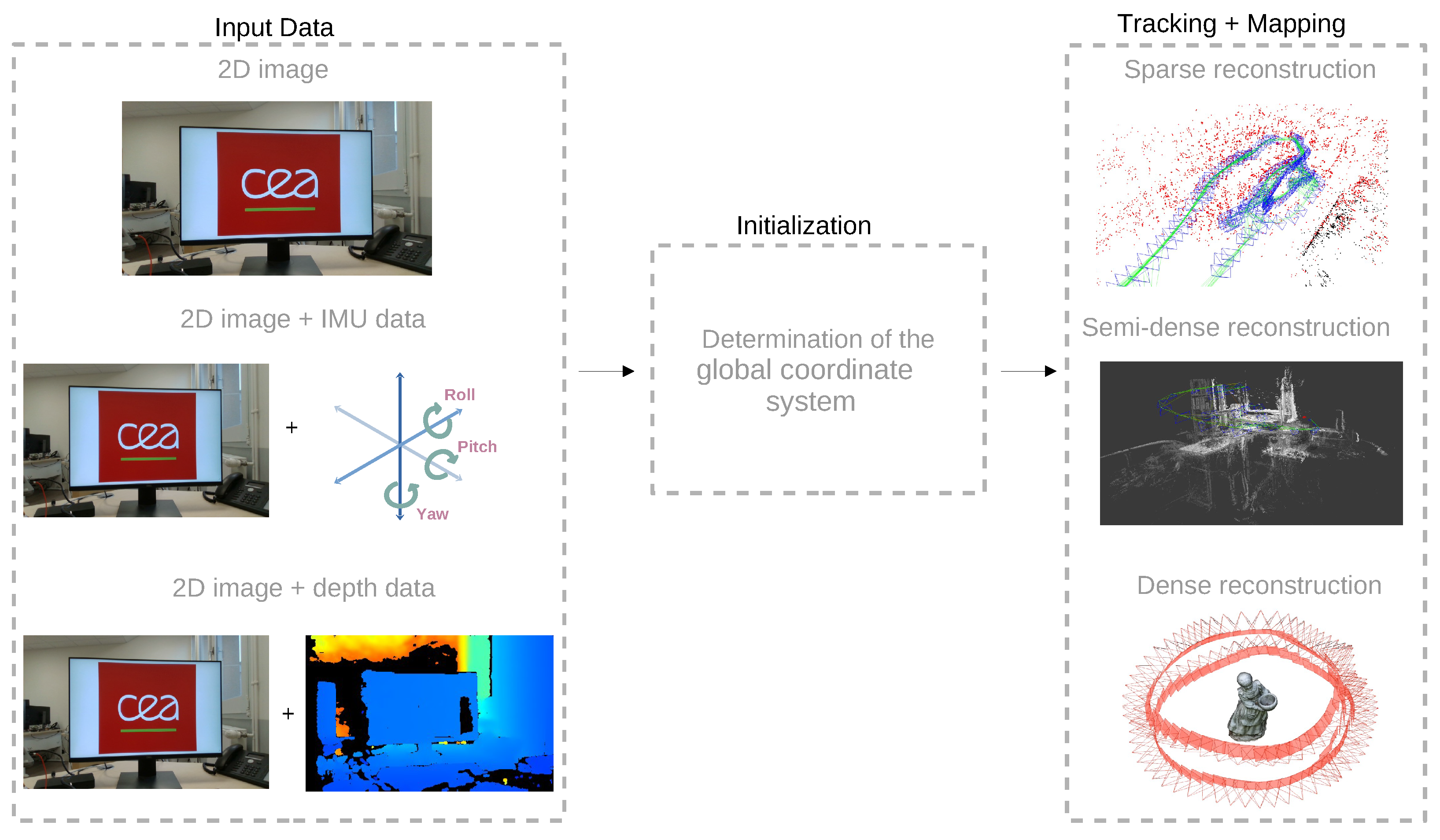
2. Visual-Based SLAM Concepts

This section presents concepts related to visual-based SLAM and odometry algorithms, and the main characteristics of the visual-based approaches covered in this paper. The visual-based SLAM techniques use one or more cameras in the sensor system, receiving 2D images as the source of information. In general, the visual-based SLAM algorithms are divided into three main threads: initialization, tracking, and mapping [10]. Figure 1 shows a general view of the three main parts generally present in visual-based SLAM approaches.
As one can see in the Figure, in visual-SLAM systems, the input can be a 2D image, both a 2D image and IMU data, or a 2D image and depth data, depending on the used approach, i.e., visual-only (Section 2.1), visual-inertial (Section 2.2), or RGB-D-based (Section 2.3), respectively. The initialization determines the global coordinates and builds an initial map, used to perform the two main steps: tracking and mapping. The tracking process is responsible for the continuous estimation of the sensor’s pose. In general, the algorithm establishes 2D–3D correspondences between the current frame and map, constituting a problem called perspective-n-points. There are several ways to solve this problem, EPnP being one of the most representative solutions [26]. The mapping process is in charge of computing and expanding the 3D structure as the camera moves. The depth data computation differs according to the employed algorithm (Section 3 addresses individually each algorithm providing detailed explanations). Finally, the mapping processes shall result in a sparse, semi-dense, or dense 3D reconstruction, according to the implemented technique.
Although we mainly refer to the concepts as belonging to the SLAM methodology, we consider, in this paper, both visual-SLAM and visual-odometry (VO) techniques, since they are closely related. The VO algorithms also seek to estimate a robot’s position through cameras as a source of information. The main difference between visual-SLAM and VO lies in considering, or not, the global consistency of the estimated trajectory and map [14]. While VO performs only local optimizations, visual-SLAM algorithms also employ loop closure detection (see Section 3), being capable of correcting drifts accumulated at the end of the robot’s trajectory.

2.1. Visual-Only SLAM

The visual-only SLAM systems are based on 2D image processing. After the images’ acquisition from more than one point of view, the system performs the initialization process to define a global coordinate system and reconstruct an initial map. In the feature-based algorithms relying on filters (filtering-based algorithms), the first step consists of initializing the map points with high uncertainty, which may converge later to their actual positions. This procedure is followed by tracking, which attempts to estimate the camera pose. Simultaneously, the mapping process includes new points in the 3D reconstruction as more unknown scenes are observed.
The visual-only SLAM system may use a monocular or stereo camera. The monocular camera-based SLAM is a well-explored domain given the small size of the sensor (the smallest of all the presented approaches), its low price, easy calibration, and reduced power consumption [27]. Despite these advantages, the monocular-based systems offer a higher complexity in system’s initialization, since at least two different views are necessary to determine an initial depth, and pose estimation and problems concerning drift and scale estimation. This last problem may be compensated by stereo cameras, which present the main advantage to feature the stereo view in only one frame. However, the sensor’s size is more significant than a simple monocular camera. In addition, it requires more processing for each frame, mainly due to the need for an image rectification process in the stereo matching stage.
The visual-only SLAM category can be divided into two main methods: feature-based and direct.

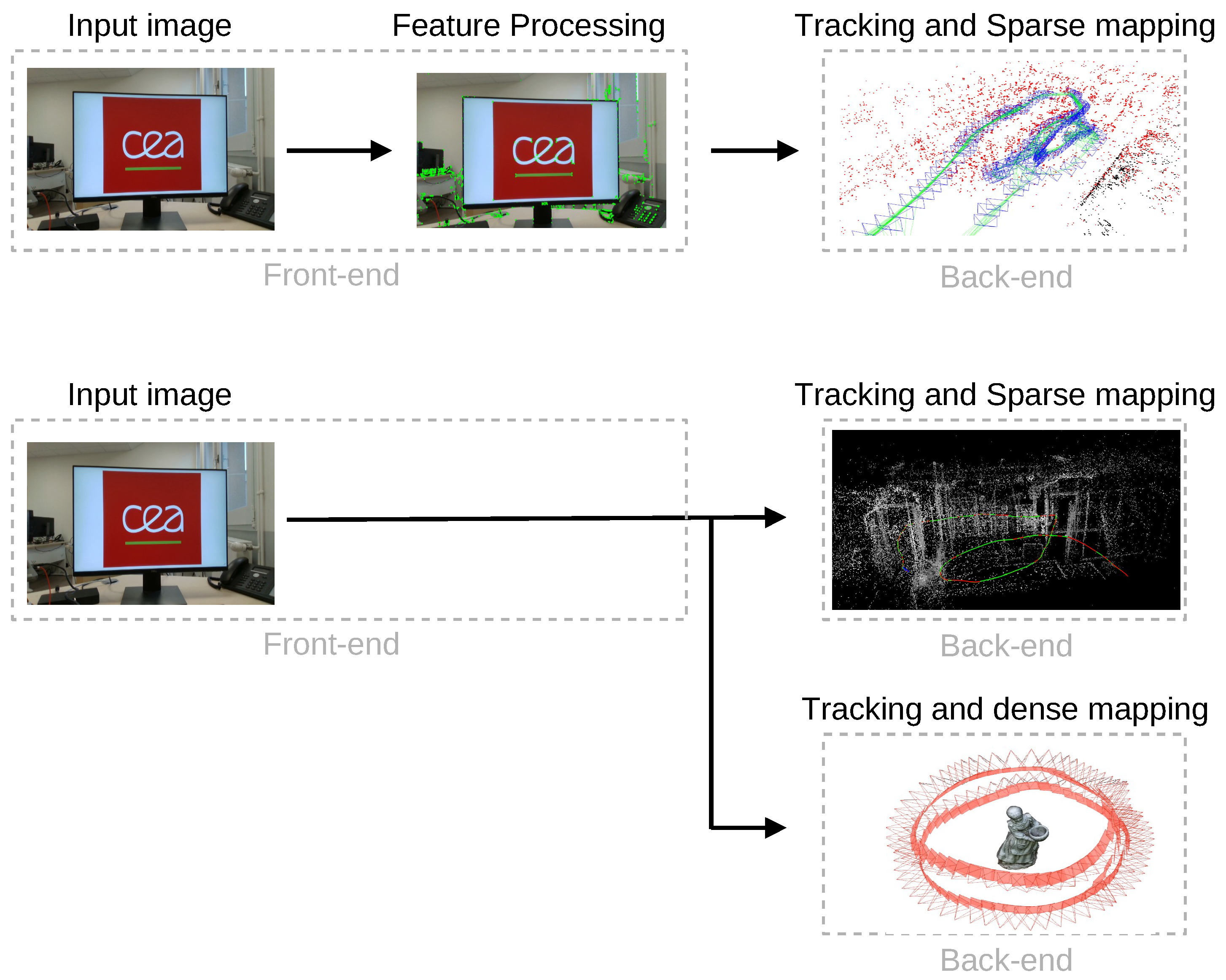
2.1.1. Feature-Based Methods

SLAM algorithms based on features consider a certain number of points of interest, called keypoints. They can be detected in several images and matched by comparing their descriptors; this process provides the camera pose estimation information. The descriptor data and keypoint location compose the feature, i.e., the data used by the algorithm to process the tracking and mapping. As the feature-based methods do not use all the frame information, they are suitable to figure in embedded implementations. However, the feature extraction may fail in a textureless environment [28], as well as it generates a sparse map, providing less information than a dense one.

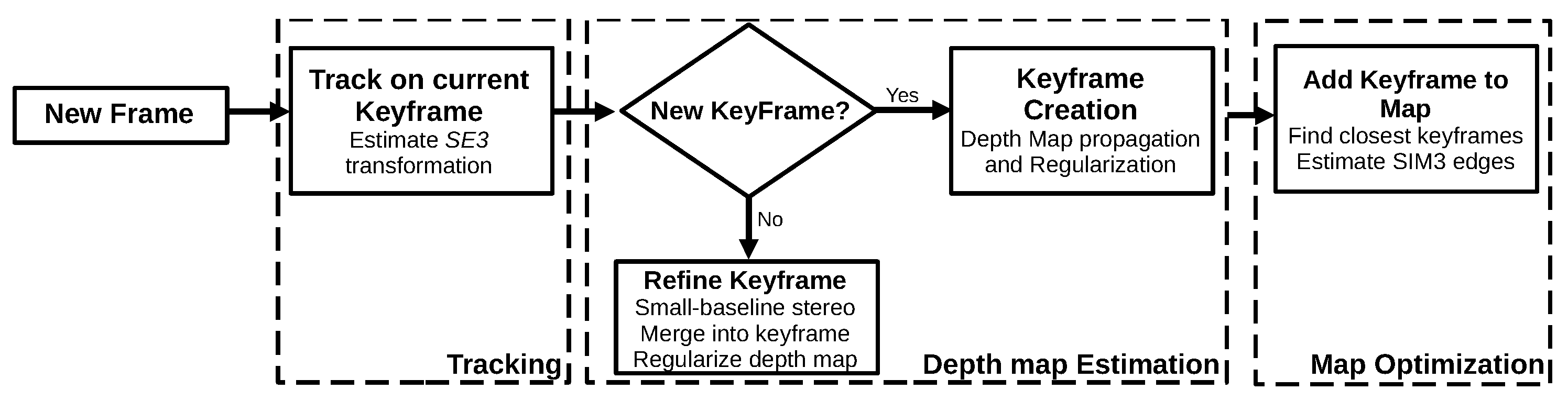
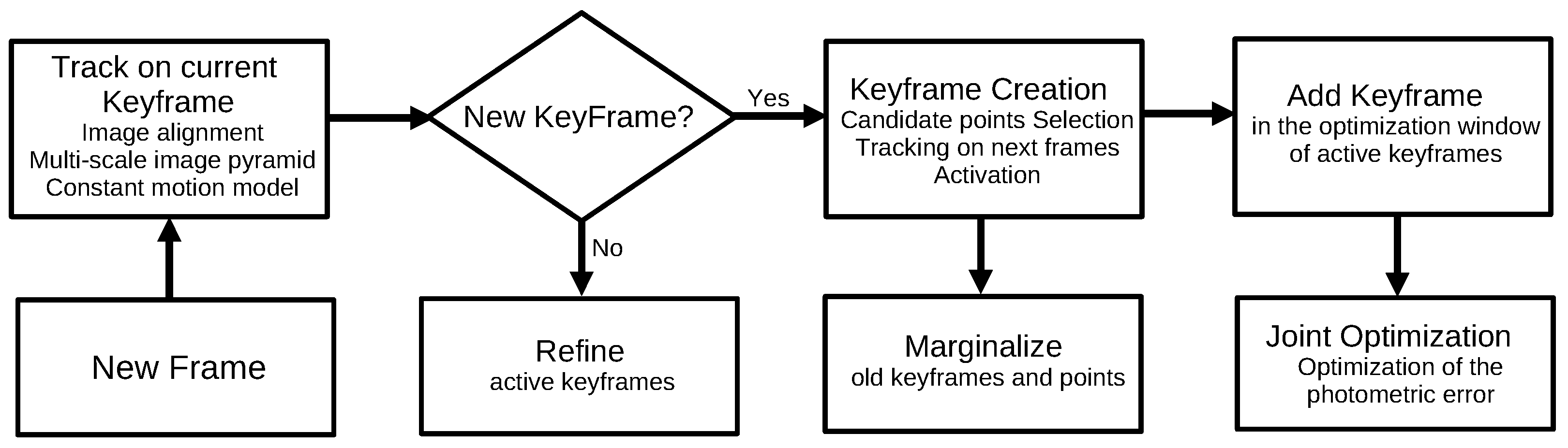
2.1.2. Direct Methods

In contrast with the feature-based methods, the direct methods use the sensor data without pre-processing, considering pixels’ intensities, and minimizing the photometric error. There are many different algorithms based on this methodology, and depending on the chosen technique, the reconstruction may be dense, semi-dense, or sparse. The reconstruction density is a substantial constraint to the algorithm’s real-time operation, since the joint optimization of both structure and camera positions is more computationally expensive for dense and semi-dense reconstructions than for a sparse one [29]. Figure 2 shows the main difference between feature-based (indirect) and direct methods according to their front-end and back-end, that is, the part of the algorithm responsible for sensor’s data abstraction and the part responsible for the interpretation of the abstracted data, respectively.

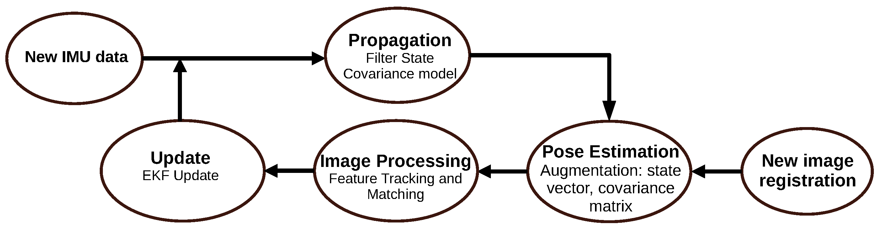
2.2. Visual-Inertial SLAM

The VI-SLAM approach incorporates inertial measurements to estimate the structure and the sensor pose. The inertial data are provided by the use of an inertial measurement unit (IMU), which consists of a combination of gyroscope, accelerometer, and, additionally, magnetometer devices. This way, the IMU is capable of providing information relative to the angular rate (gyroscope) and acceleration (accelerometer) along the x-, y-, and z-axes, and, additionally, the magnetic field around the device (magnometer). While adding an IMU may increase the information richness of the environment and provide higher accuracy, it also increases the algorithm’s complexity, especially during the initialization step, since, besides the initial estimation of the camera pose, the algorithm also has to estimate the IMU poses. VI-SLAM algorithms can be divided according to the type of fusion between the camera and IMU data, which can be loosely or tightly coupled. The loosely coupled methods do not merge the IMU states to estimate the full pose: instead, the IMU data are used to estimate the orientation and changes in the sensor’s position [18]. On the other side, the tightly coupled methods are based on the fusion of camera and IMU data into a motion equation, resulting in a state estimation that considers both data.
In addition, VI-SLAM algorithms present different implementations according to their back-end approach, which can be filtering-based or optimization-based. The front-end of filtering-based approaches for VI-SLAM relies on feature extraction, while optimization-based methods (also known as keyframe-based approaches) rely on global optimizations, which increase the system’s accuracy, as well as the algorithm’s computational cost.

2.3. RGB-D SLAM

SLAM systems based on RGB-D data started to attract more attention with the advent of Microsoft’s Kinect in 2010. RGB-D sensors consist of a monocular RGB camera and a depth sensor, allowing SLAM systems to directly acquire the depth information with a feasible accuracy accomplished in real-time by low-cost hardware. As the RGB-D devices directly provide the depth map to the SLAM systems, the general framework of SLAM based on this approach differs from the other ones already presented.
Most of the RGB-D-based systems make use of the iterative closest point (ICP) algorithm to locate the sensor, fusing the depth maps to obtain the reconstruction of the whole structure. RGB-D systems present advantages such as providing color image data and dense depth map without any pre-processing step, hence decreasing the complexity of the SLAM initialization [10]. Despite this, this approach is most suitable to indoor environments, and requires large memory and power consumption [32].

3. Visual-SLAM Algorithms

Each considered approach presented in Section 2 includes several algorithms, making it difficult to select the most suitable SLAM or odometry algorithm according to one’s project constraints. Therefore, we present the most representative algorithms of each approach, selected based on literature feedback, to accomplish a brief review of each one, and a systematic analysis based on six selected criteria that, in general, are presented as limiting factors of SLAM projects. Besides the proposed criteria, it is also necessary to characterize the scene and application, since some scenarios may present specific attributes that may imply specific evaluation criteria, such as the analysis presented in [33]. The authors consider the autonomous driving application characteristics, which implies a set of specific criteria, such as the required accuracy, scalability, dynamicity, etc. Thus, considering the general approach of the SLAM systems, we established six criteria that influence system dimensioning, accuracy, and hardware implementation. They are: algorithm type, map density, global optimization, loop closure, availability, and embedded implementations:
  • Algorithm type: this criterion indicates the methodology adopted by the algorithm. For the visual-only algorithms, we divide them into feature-based, hybrid, and direct methods. Considering the visual-inertial algorithms, they must be filtering-based or optimization-based methods. Lastly, the RGB-D approach can be divided concerning their tracking method, which can be direct, hybrid, or feature-based.
  • Map density: in general, dense reconstruction requires more computational resources than a sparse one, having an impact on memory usage and computational cost. On the other hand, it provides a more detailed and accurate reconstruction, which may be a key factor in a SLAM project.
  • Global optimization: SLAM algorithms may include global map optimization, which refers to the technique that searches to compensate the accumulative error introduced by the camera movement, considering the consistency of the entire structure.
  • Loop closure: the loop closing detection refers to the capability of the SLAM algorithm to identify the images that were previously detected by the algorithm to estimate and correct the drift accumulated during the sensor movement.
  • Availability: several SLAM algorithms are open source and made available by the authors or have their implementations made available by third parties, facilitating their usage and reproduction.
  • Embedded implementations: the embedded SLAM implementation is an emerging field used in several applications, especially in robotics and automobile domains. This criterion depends on each algorithm’s hardware constraints and specificity, since there must be a trade-off between algorithm architecture in terms of energy consumption, memory, and processing usage. We assembled the main publications we found presenting fully embedded SLAM systems in platforms such as microcontrollers and FPGA boards.
In the following, we present the selected SLAM algorithms considered the most representative of each of the three presented approaches according to their publication years.

3.1. Visual-Only SLAM

The selected visual-only SLAM algorithms are presented in Figure 3 and explained in the following subsections.

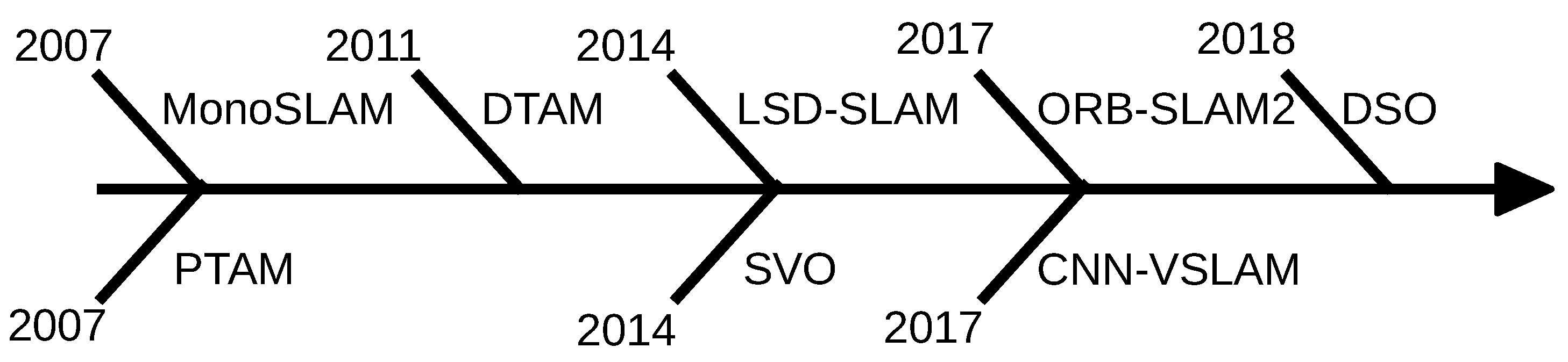
3.1.1. MonoSLAM (2007)

The first monocular SLAM algorithm is MonoSLAM, which was proposed by Davidson et al. [27] in 2007. The first step of the algorithm consists of the system’s initialization. Then, it updates the state vector considering a constant velocity motion model, where the camera motion and environment structure are estimated in real-time using an extended Kalman filter (EKF). The algorithm is represented by Figure 4. MonoSLAM operates in real-time and was made available by the authors. Moreover, since MonoSLAM is based on EKF, an already well-covered topic, several embedded implementations based on this algorithm are found in the literature. In [34,35], Vincke et al. based their implementation on the MonoSLAM algorithm, combining multiple sensors and a multi-processor architecture to evaluate its implementation. In [34], the authors used an ARM + DSP + GPU architecture (OMAP3530 architecture) to implement the localization, reconstruction, and feature detection. They combine this architecture with a co-processor ATMega168 used for data pre-processing and robot controlling. In [35], they based the architecture on a combination of multi-CPUs + GPUs provided by the use of an OMAP4430 architecture. The authors implemented the different tasks of the algorithms into both single-core and dual-core ARM architecture, and compared their performances. In addition, they parallelized the matching and initialization tasks using the ARM and NEON processors provided by the OMAP4430.
MonoSLAM requires a known target for the initialization step, which is not always accessible. In addition, the algorithm’s complexity increases proportionally with the size of the environment. This algorithm neither employs global optimization techniques nor loop closure detection. At last, it only reconstructs a map of landmarks, which may be a drawback regarding the applications that require a more accurate reconstruction.

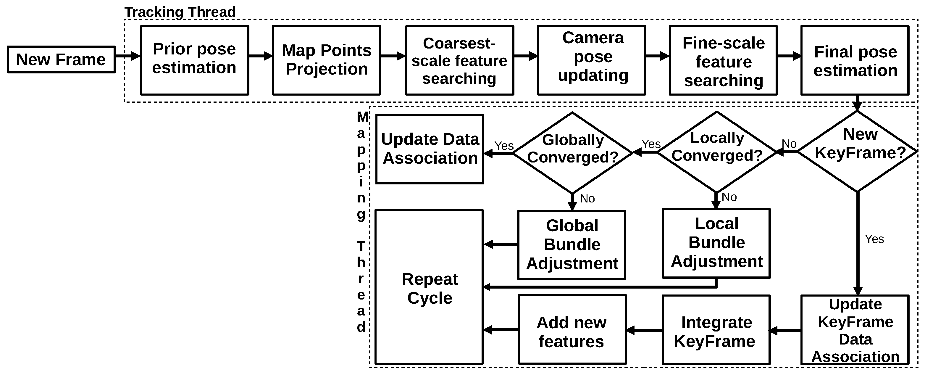
3.1.2. Parallel Tracking and Mapping (2007)

Another pioneer algorithm is the Parallel Tracking and Mapping (PTAM) [36] algorithm. PTAM was the first algorithm to separate Tracking and Mapping into two different threads and to apply the concept of keyframes to the mapping thread. First, the mapping thread performs the map initialization. New keyframes are added to the system as the camera moves and the initial map is expanded. Triangulation between two consecutive keyframes calculates the new point’s depth information. The tracking thread computes the camera poses, and for each new frame, it estimates an initial pose for performing the projection of the map points on the image. PTAM uses the correspondences to compute the camera pose by minimizing the reprojection error. Figure 5 represents the steps performed by the PTAM algorithm.
PTAM allows the map representation by a large number of features and performs global optimization. Despite these advantages, the PTAM algorithm presents a high complexity due to the bundle adjustment step. In addition, it does not count with loop closure, and the generated map is more suitable to identify landmarks. Furthermore, it requires the user’s interaction to establish the initial keyframes, and it presents a non-negligible power consumption, which makes it unsuitable for low-cost embedded systems [37].

3.1.3. Dense Tracking and Mapping (2011)

Dense tracking and mapping (DTAM), proposed by Newcombe et al. [38], was the first fully direct method in the literature. The algorithm is divided into two main parts: dense Mapping and dense tracking. The first stage searches to estimate the depth values by defining data cost volume representing the average photometric error of multiple frames computed for the inverse depth of the current frame. The inverse depth that minimizes the photometric error is selected to integrate the reconstruction. In the dense tracking stage, DTAM estimates the motion parameters by aligning an image from the dense model projected in a virtual camera and the current frame. Figure 6 shows a general view of the DTAM algorithm. The algorithm provides an accurate and detailed reconstruction, but this level of density reconstruction impacts the computational cost to store and process the data. As a consequence, to achieve real-time operation, the algorithm requires state-of-the-art GPUs [10]. The authors in [39] employed a CPU + GPU architecture of different iPhone models to implement a fully dense algorithm based on DTAM. They used the CPU for the tracking task and the GPU for depth estimation and frame fusion. DTAM does not implement loop closure techniques or global optimization.

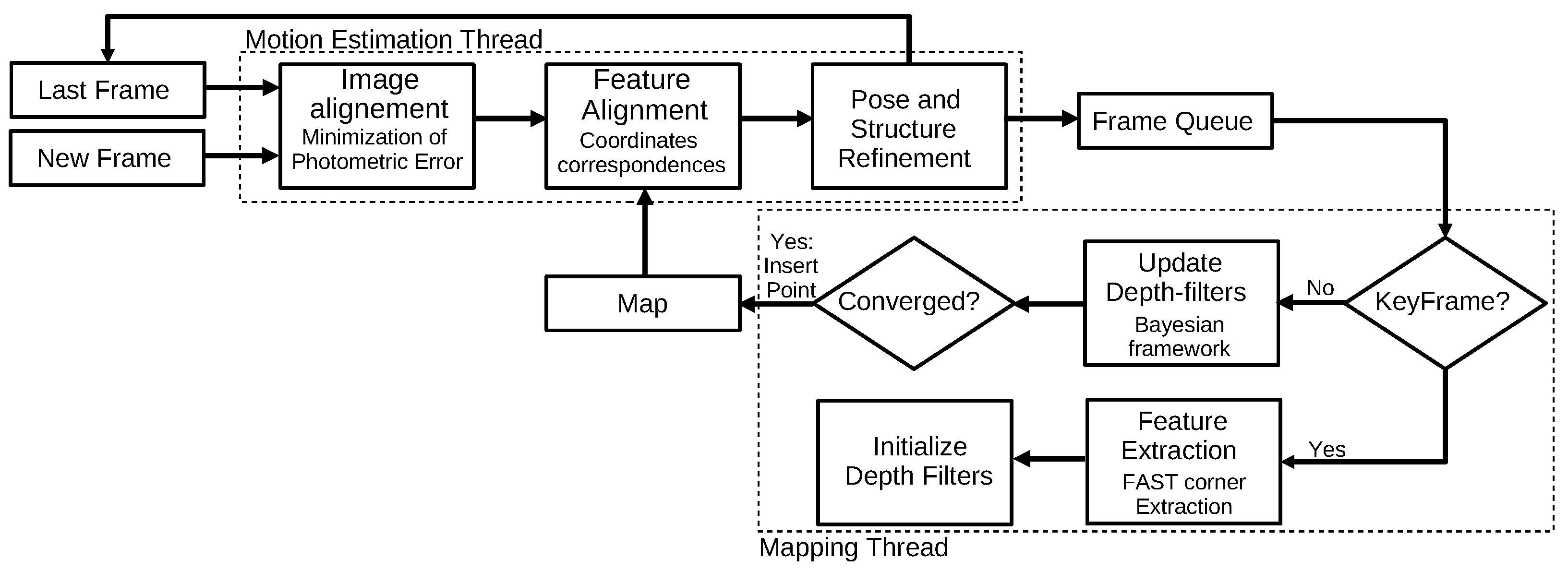
3.1.4. Semi-Direct Visual Odometry (2014)

The semi-direct visual odometry (SVO) algorithm [40] combines the advantages of both feature-based and direct methods. The algorithm is divided into two main threads: motion estimation and mapping. The first thread searches to estimate the sensor’s motion parameters, which consists of minimizing the photometric error. The mapping thread is based on probabilistic depth filters, and it searches to estimate the optimum depth value for each 2D feature. When the algorithm achieves a low uncertainty, it inserts the 3D point in the reconstruction, as shown in Figure 7. SVO enables direct pixel correspondences and the usage of a probabilistic mapping method. In addition, the algorithm is capable of operating with a high frame rate, since it does not need to extract features for every frame [41], which enables its operation in a low-cost embedded system, as with the embedded platform considered by [40] that consists in an Odroid-U2. Nonetheless, SVO presents a limited accuracy due to the short-term data association [22]. SVO does not implement global optimization techniques or loop closure. The authors already proposed an extended version of the SVO, SVO 2.0 [42], in which the algorithm is capable of processing stereo data and IMU information.

3.1.5. Large-Scale Direct Monocular SLAM (2014)

The large-scale direct monocular SLAM (LSD-SLAM) [24] is a direct algorithm that performs a semi-dense reconstruction. The algorithm consists of three main steps: tracking, depth map estimation, and map optimization. The first step minimizes the photometric error to estimate the sensor’s pose. Next, the LSD-SLAM performs the keyframe selection in the depth map estimation step. If it adds a new keyframe to the algorithm, it initializes its depth map; otherwise, it refines the depth map of the current keyframe by performing several small-baseline stereo comparisons. Finally, in the map optimization step, the LSD-SLAM incorporates the new keyframe in the map and optimizes it by applying a pose–graph optimization algorithm. Figure 8 illustrates the procedure. This technique allows the real-time construction of large-scale maps and employs global optimization and loop closure. In addition, by combining the absence of feature extraction, characteristic of the direct methods, with a semi-dense reconstruction, this method improves its efficiency, enabling embedded implementations. Boikos and Christos-Savvas in [29,43] used CPU + FPGA architectures to implement the LSD-SLAM algorithm. In [29], the authors implemented two accelerators on the FPGA to perform more expensive tasks of the tracking thread; that is, Jacobian calculations, as well as residual and weight calculations. The ARM CPU was used to implement the other tasks of the algorithm. In [43], the authors implement the direct tracking thread on the FPGA, while the CPU was responsible for memory, hardware control, and parameter setup. The LSD-SLAM map estimation is based essentially on pose-graph optimization [22] and the algorithm achieved lower accuracy than others, such as PTAM and ORB-SLAM [41].

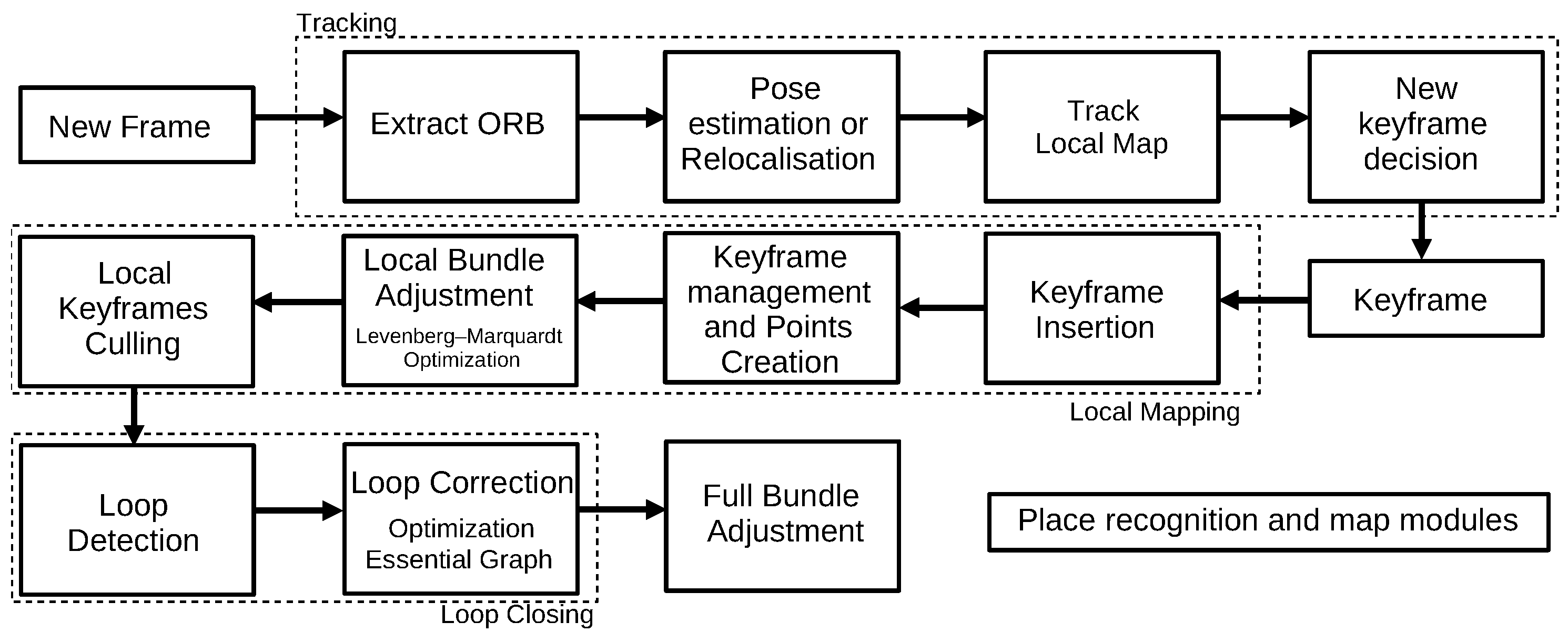
3.1.6. ORB-SLAM 2.0 (2017)

The ORB-SLAM2 algorithm [44], originated from ORB-SLAM [41], is considered the state of the art of feature-based algorithms. It works in three parallel threads: tracking, local mapping, and loop closing. The first thread locates the sensor by finding features correspondences and minimizing the reprojection error. The local mapping thread is responsible for the map management operations. The last thread, loop closing, is in charge of detecting new loops and correcting the drift error in the loop. After processing the three threads, the algorithm also considers the whole structure and estimated motion consistency by performing a full bundle adjustment. Figure 9 represents the threads that constitute the algorithm. ORB-SLAM2 considers the monocular, stereo and RGB-D approaches, and implements global optimization and loop closure techniques. Nonetheless, the tracking failure situation may lead to a lost state if the system does not recognize a high-similarity frame [45]. In addition, this method needs to acquire the images with the same frame rate as it processes them, which makes real-time operation in embedded platforms difficult [46]. This is in spite of the fact that several embedded implementations may be found in the literature. Yu et al. [47] used a CPU to run the ORB-SLAM algorithm and Abouzahir et al. [46] implemented the algorithm in different CPU- and GPU-based platforms, and evaluated the performance of each thread on the platforms.

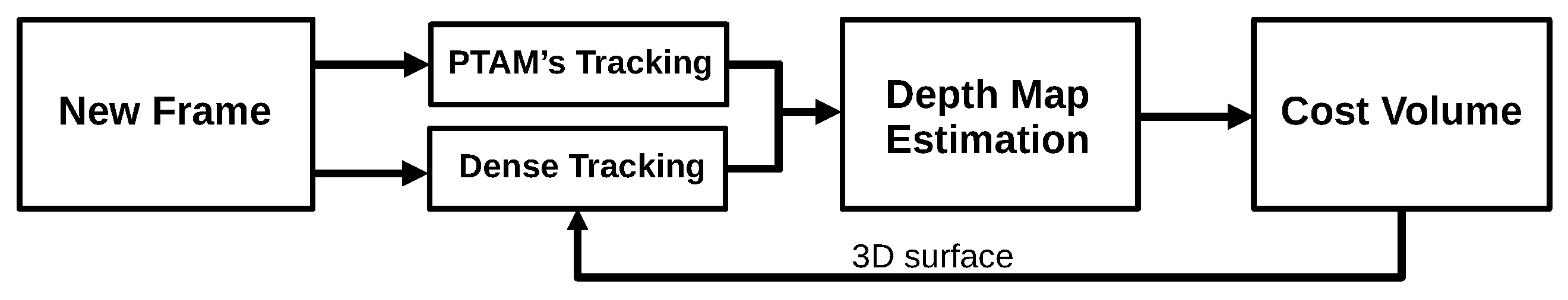
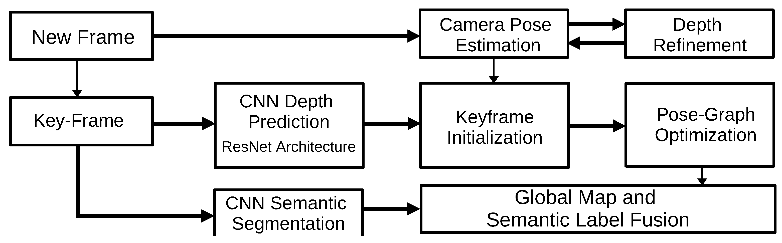
3.1.7. CNN-SLAM (2017)

CNN-SLAM [48] is one of the first works to present a real-time SLAM system based on convolutional neural networks (CNN). The algorithm may be divided into two different pipelines: one applied in every input frame and another in every keyframe. The first is responsible for the camera pose estimation by minimizing the photometric error between the current frame and the nearest keyframe. In parallel, for every keyframe, the depth is predicted by a CNN. In addition, the algorithm predicts the semantic segmentation for each frame. After these processing steps, the algorithm performs a pose-graph optimization to obtain a globally optimized pose estimation, as shown in Figure 10.
This algorithm does not suffer from absolute scale limitation, since it uses depth prediction to perform the scale estimation [48]. In addition, it counts with global optimization and loop closure. The authors needed to employ a CPU+GPU architecture to run the algorithm in real-time.

3.1.8. Direct Sparse Odometry (2018)

The direct sparse odometry (DSO) algorithm [31] combines a direct approach with a sparse reconstruction. The DSO algorithm considers a window of the most recent frames. It performs a continuous optimization by applying a local bundle adjustment that optimizes the keyframes window and the inverse depth map. The algorithm divides the image into several blocks and selects the highest intensity points. The DSO considers exposure time and lens distortion in the optimization to increase the algorithm’s robustness. Initially, this algorithm does not include global optimization or loop closure, but Xiang et al. [49] proposed an extension of the DSO algorithm, including loop closure detection and pose-graph optimization. The DSO main steps are represented in Figure 11.

3.1.9. General Comments

In this Section, we presented the main visual-only-based SLAM algorithms. Table 1 summarizes the main characteristics and analyzed criteria for the presented visual-only SLAM algorithms.
The main benefits and drawbacks of each method were individually addressed. Considering a general point of view, the visual-only-based SLAM algorithms may be considered a well-explored field, since most of the algorithms were made available by the authors, which also had consequences for the embedded SLAM implementations found in the literature. The embedded implementations presented in Table 1 consider the full SLAM algorithms implementation and works that do not perform essential modifications in the originally proposed technique. However, it is possible to find in the literature several embedded implementations based on fundamental concepts of the presented algorithms. For instance, the MonoSLAM principles have been used for the development and implementation of several other SLAM on SoC implementations, such as the heterogeneous architecture recently proposed by Piat et al. [59]. Furthermore, the growing development of the CNN-based SLAM algorithms can be noticed. Besides the presented CNN-SLAM, other algorithms are found in the literature, such as the CNN-SVO [28] algorithm that uses depth prediction to initialize the depth filters. Developments of the hardware implementations of CNN-based SLAM algorithms have been growing since the launch of the AI accelerator Xilinx Deep-learning Processor Unit [60] in 2019. This hardware already enabled the progress on embedded implementations of CNN-based algorithms: one example is the work presented in [61] that uses an FPGA platform to perform a CNN-based feature extractor.

3.2. Visual-Inertial SLAM

A timeline representing the selected visual-inertial algorithms is presented in Figure 12 and the algorithms are explained in the following subsections.

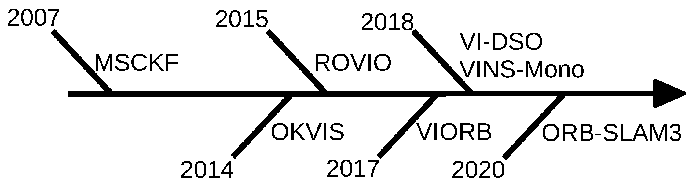
3.2.1. Multi-State Constraint Kalman Filter (2007)

The multi-state constraint Kalman filter (MSCKF) [62] can be implemented using both monocular and stereo cameras [63]. The algorithm’s pipeline consists of three main steps: propagation, image registration, and update. In the first step, the MSCKF considers the discretization of a continuous-time IMU model to obtain the propagation of the filter state and covariance. Then, the image registration performs the state augmentation each time a new image is recorded. This estimation is added in the state and covariance matrix to initiate the image processing module (feature extraction). Finally, the algorithm performs the filter update. Figure 13 represents the algorithm. The MSCKF is considered one of the fastest filter-based methods in the literature [64], a consequence of its low computational cost [63], which makes this algorithm suitable for embedded implementations. Delmerico and Scaramuzza [65] used different hardware platforms based on CPU architectures to implement visual-inertial SLAM algorithms. The authors implemented the algorithm in three different embedded boards—Intel NUC, Up Board, and ODROID. However, the Jacobian calculations performed by the algorithm may cause inconsistency and loss of accuracy [66].

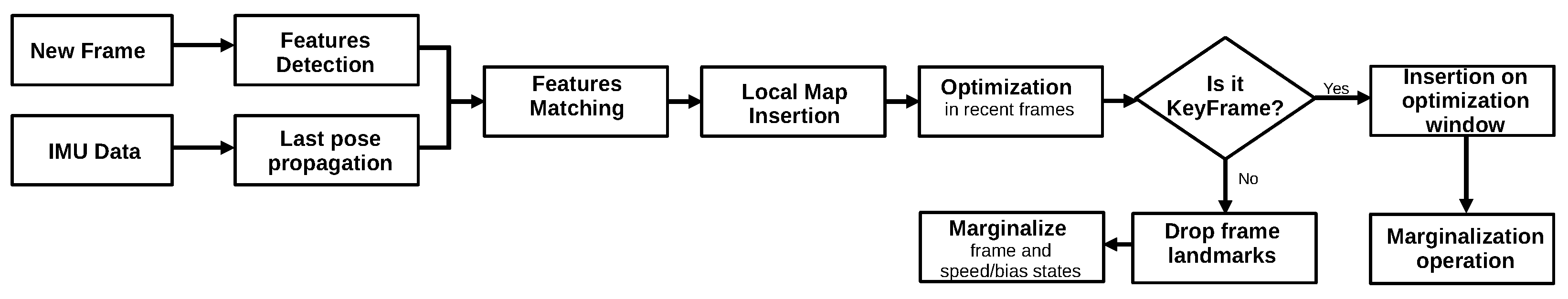
3.2.2. Open Keyframe-Based Visual-Inertial SLAM (2014)

Open Keyframe-based Visual-Inertial SLAM (OKVIS) [67] is an optimization-based method. It combines the IMU data and reprojection terms into an objective function, allowing the algorithm to jointly optimize both the weighted reprojection error and temporal error from IMU. The algorithm builds a local map, and then the subsequent keyframes are selected according to the keypoints match area. The algorithm can be depicted as shown in Figure 14. The OKVIS algorithm presented a lower memory usage when compared with other algorithms (this will be explained in the following subsections), such as VINS-Mono, VIORB, and ROVIO [18], enabling its embedded implementation. Already mentioned, the work of Delmerico and Scaramuzza [65] used different CPU platforms to implement the OKVIS algorithm. However, to achieve real-time performance in the Up Board and ODROID, the authors needed to reduce the number of keypoints, the keyframe window, and the IMU-linked frames. Nikolic et al. [68] used an FPGA-CPU architecture to evaluate the OKVIS algorithm’s performance. The authors took advantage of the logic blocks on the FPGA to implement the image processing techniques and accelerated the keypoint detection process. However, it was demonstrated that the algorithm is less accurate than others [18].

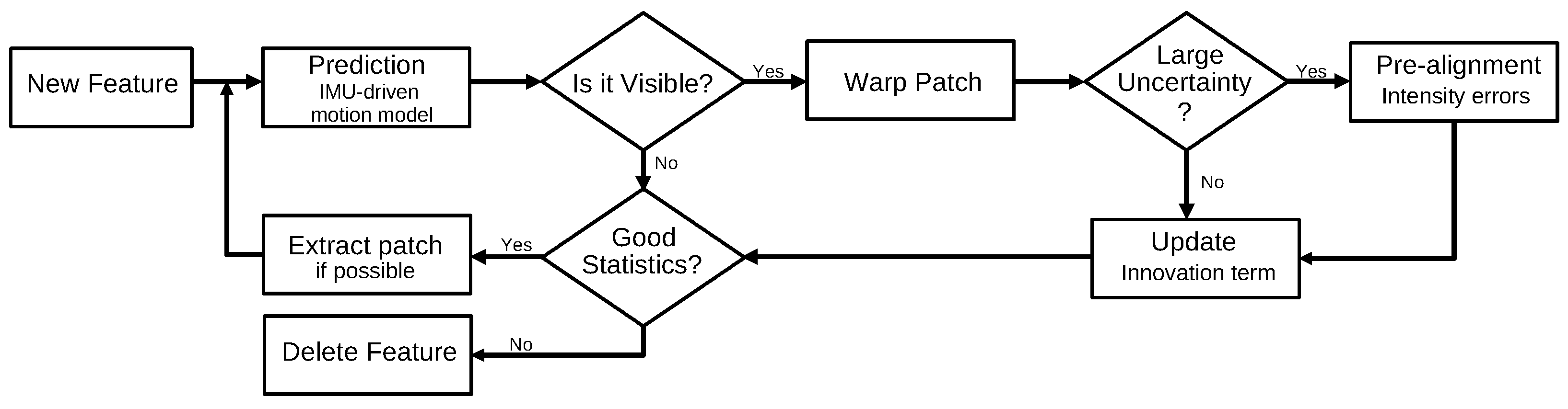
3.2.3. Robust Visual Inertial Odometry (2015)

The Robust Visual Inertial Odometry (ROVIO) algorithm [69] is another filter-based method that uses the EKF approach, and similar to other filter-based methods, it uses the IMU data to state propagation, and the camera data to filter update. However, besides performing the feature extraction, ROVIO executes the extraction of multi-level patches around the features, as illustrated by Figure 15. The patches are used by the prediction and update step to obtain the innovation term, i.e., the calculation of the error between the frame and the projection of the multi-level patch into the frame. The ROVIO algorithm achieves good accuracy and robustness under a low resource utilization [18,65], being suitable for embedded implementations [65]. However, the algorithm proved to be more sensitive to per-frame processing time [65] and less accurate than other algorithms, such as VI-DSO [70].

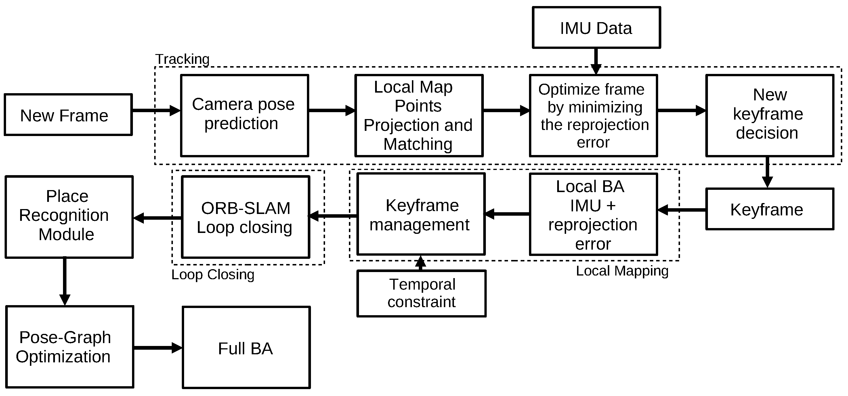
3.2.4. Visual Inertial ORB-SLAM (2017)

The Visual-Inertial ORB-SLAM (VIORB) algorithm [71] is based on the already presented ORB-SLAM algorithm [44]. As such, the system also counts with three main threads: tracking, local mapping, and loop closing. In VIORB, the tracking thread estimates the sensor pose, velocity, and IMU biases. Additionally, this thread performs the joint optimization of the reprojection error of the matched points and IMU error data. The local mapping thread adopts a different culling policy considering the IMU operation. Finally, the loop closing thread implements a place recognition module to identify the keyframes already visited by the sensors. Furthermore, the algorithm performs an optimization to minimize the accumulated error. Figure 16 seeks to illustrate the main differences between the ORB-SLAM algorithm (see Figure 9) and its visual-inertial version. The VIORB algorithm was the first visual-inertial method to employ map reuse, and it presents high-performance accuracy [64,70,72] and memory usage [18]. Nonetheless, the IMU initialization takes between 10 to 15 s [71], and no embedded implementations were found. In [22], the authors propose the ORB-SLAM3 algorithm, which is based on ORB-SLAM2 and VIORB algorithms. The system presents a reduced initialization time compared to its predecessor, VIORB.

3.2.5. Monocular Visual-Inertial System (2018)

Monocular Visual-Inertial System (VINS-Mono) [73] is a monocular visual-inertial state estimator. It starts with a measurement process responsible for features extraction and tracking, and a pre-integration of the IMU data between the frames. Then, the algorithm performs an initialization process to provide the initial values for a non-linear optimization process that minimizes the visual and inertial errors. The VINS also implements a relocalization and a pose-graph optimization module that merges the IMU measurements and features observations. Figure 17 illustrates the VINS-Mono algorithm. The algorithm can also be applied considering binocular and stereo approaches [74]. The VINS-Mono already demonstrated to achieve high accuracy when compared to other algorithms. Yet, it presented the highest memory usage when compared to algorithms such as ROVIO, VIORB, and OKVIS [18]. This is despite the fact that, since it only considers pose and velocity from the latest IMU states during the optimization process, this algorithm still demonstrated its suitability in embedded implementations [73].

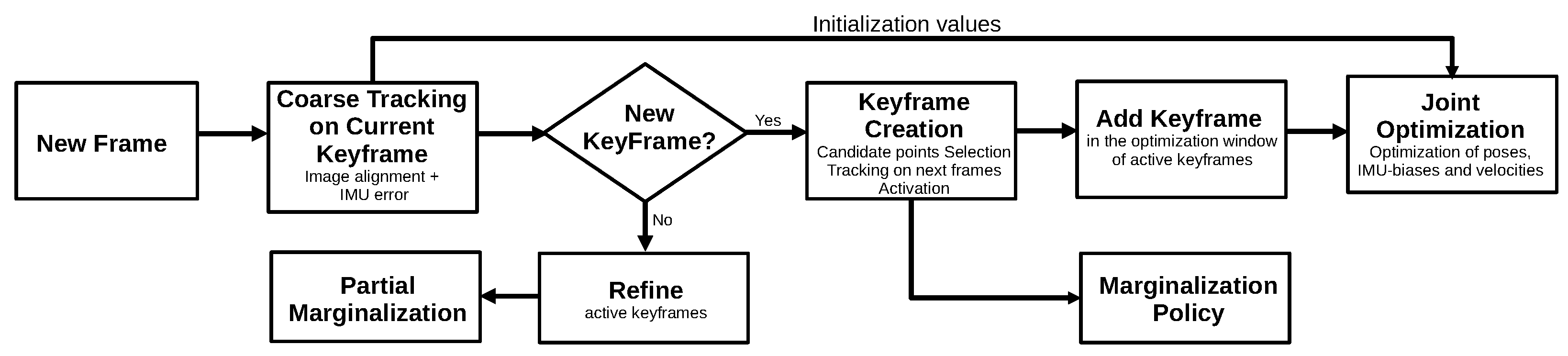
3.2.6. Visual-Inertial Direct Sparse Odometry (2018)

The Visual-Inertial Direct Sparse Odometry (VI-DSO) algorithm [70] is based on the already presented DSO algorithm [31]. The algorithm searches to minimize an energy function that combines the photometric and inertial errors, which is built considering a nonlinear dynamic model. Figure 18 shows an overview of the VI-DSO algorithm that illustrates its main differences concerning the DSO technique. The VI-DSO is an extension of DSO that considers the inertial information, which results in better accuracy and robustness than the original DSO and other algorithms, like ROVIO [70]. However, the initialization procedure relies on bundle adjustment, which makes the initialization slow [22]. The algorithm does not perform global optimization and loop closure detection, and embedded implementations were not found in the literature.

3.2.7. ORB-SLAM3 (2020)

The already mentioned ORB-SLAM3 algorithm [75] is a technique that combines the ORB-SLAM and VIORB algorithms. As with its predecessors, the algorithm is divided into three main threads: tracking, local mapping and, instead of loop closing, loop closing and map merging. In addition, ORB-SLAM3 maintains a multi-map representation called Atlas, which maintains an active map used by the tracking thread, and non-active maps used for relocalization and place recognition. The first two threads follow the same principle as VIORB, while map merging is added to the last thread. The loop closing and map merging thread uses all the maps in Atlas to identify common parts and perform loop correction or merge maps and change the active map, depending on the location of the overlapped area. Another important aspect of ORB-SLAM3 concerns the proposed initialization technique that relies on the Maximum-a-Posteriori algorithm individually applied to the visual and inertial estimations, which are later jointly optimized. This algorithm can be used with monocular, stereo, and RGB-D cameras, and implements global optimizations and loop closures techniques. However, authors in [76] demonstrated significant errors results of ORB-SLAM3 online performance. In [77], the algorithm obtained a good performance, but failed to process all the sequences, and obtained inaccurate estimates in outdoor sequences.

3.2.8. General Comments

This Section presented seven main visual-inertial SLAM algorithms, as long as an individual analysis of each of them. Table 2 summarizes the main characteristics and analyzed criteria for the presented visual-inertial SLAM algorithms.
In a general analysis, the addition of an IMU to visual-based SLAM algorithms has the primary purpose of increasing the system’s robustness, which was already demonstrated to be true [2,22,70]. We observed greater literature feedback from the algorithms made available by their authors, which directly influenced the embedded implementations found in the literature. Unlike its visual-only version, we did not find an embedded version of the VIORB algorithm, since the original article does not provide an open-source version, and the more recent one, the open-source ORB-SLAM3, was recently published in 2020 [22]. As for the inertial version of the DSO algorithm, the authors do not provide an open-source implementation; however, an implementation by third parties may be found [83], even though it requires optimization. The visual-inertial SLAM-based approaches represent a growing field, and several recent articles have been published, combining the IMU technologies with a large variety of sensors [85,86,87]. Limiting our research to the visual-SLAM techniques, we could find several articles proposing solutions to increase the performance of the VI-based SLAM algorithm’s initialization step [75,88,89].

3.3. RGB-D SLAM

The most representative SLAM algorithms based on RGB-D sensors, i.e., considering RGB images and depth information directly, are presented in Figure 19, according to their published years, and explained in the following subsections.

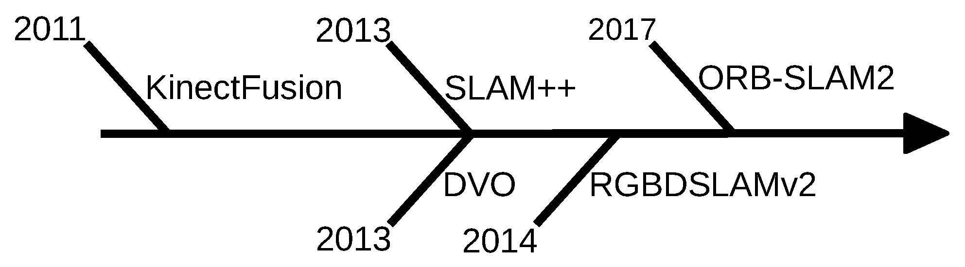
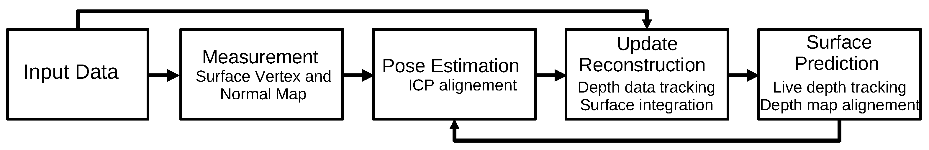
3.3.1. KinectFusion (2011)

The KinectFusion algorithm [90] was the first algorithm based on an RGB-D sensor to operate in real-time. The algorithm includes four main steps: the measurement, pose estimation, reconstruction update, and surface prediction. In the first step, the RGB image and depth data are used to generate a vertex and a normal map. In the pose estimation step, the algorithm applies the ICP alignment between the current surface and the predicted one (provided by the previous step). Then, the reconstruction update step integrates the new depth frame into the 3D reconstruction, which is raycasted into the new estimated frame to obtain a new dense surface prediction. The KinectFusion algorithm is capable of good mapping in maximum medium-sized rooms [90]. However, it accumulates drift errors, since it does not perform loop closing [91]. Nardi et al., in [92], propose an implementation for the KinectFusion and test it in different CPU- and GPU-based platforms. Bodin et al. [93] use the framework proposed by [92] to implement the KinectFusion in two different CPU and GPU platforms. An overview of the steps performed by the algorithm is shown in Figure 20.

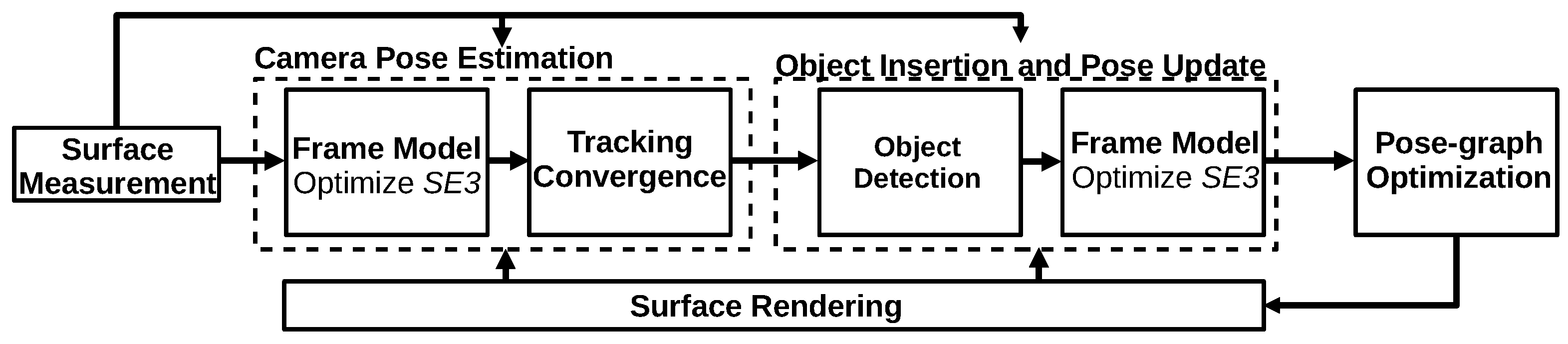
3.3.2. SLAM++ (2013)

The SLAM++ algorithm [94] is an object-oriented SLAM algorithm that takes advantage of previously known scenes containing repeated objects and structures, such as a classroom. After the system initialization, SLAM++ operates in four steps: camera pose estimation, object insertion, and pose update, pose–graph optimization, and surface rendering. The first step estimates the current camera pose by applying the ICP algorithm, considering dense multi-object prediction in the current SLAM graph. Next, the algorithm searches to identify objects in the current frame using the database information. The third step inserts the considered objects in the SLAM graph by performing a pose–graph optimization operation. Finally, the algorithm renders the objects in the graph, as shown in Figure 21. SLAM++ performs loop closure detection and, by considering the object’s repeatability, it increases its efficiency and scene description. Nevertheless, the algorithm is most suitable for already known scenes.

3.3.3. Dense Visual Odometry (2013)

The dense visual odometry SLAM (DVO-SLAM) algorithm, proposed by Kerl et al. [95], is a keyframe-based technique. It minimizes the photometric error between the keyframes to acquire the depth values and pixels coordinates, as well as camera motion. The algorithm calculates, for each input frame, an entropy value that is compared to a threshold value. The same principle is used for loop detection, although it uses a different threshold value. The map is represented by a SLAM graph where the vertex has camera poses, and edges are the transformations between keyframes. This algorithm is robust to textureless scenes and performs loop closure detection. The map representation relies on a representation of the keyframes, and the algorithm does not perform an explicit map reconstruction. Figure 22 shows an overview of the DVO algorithm.

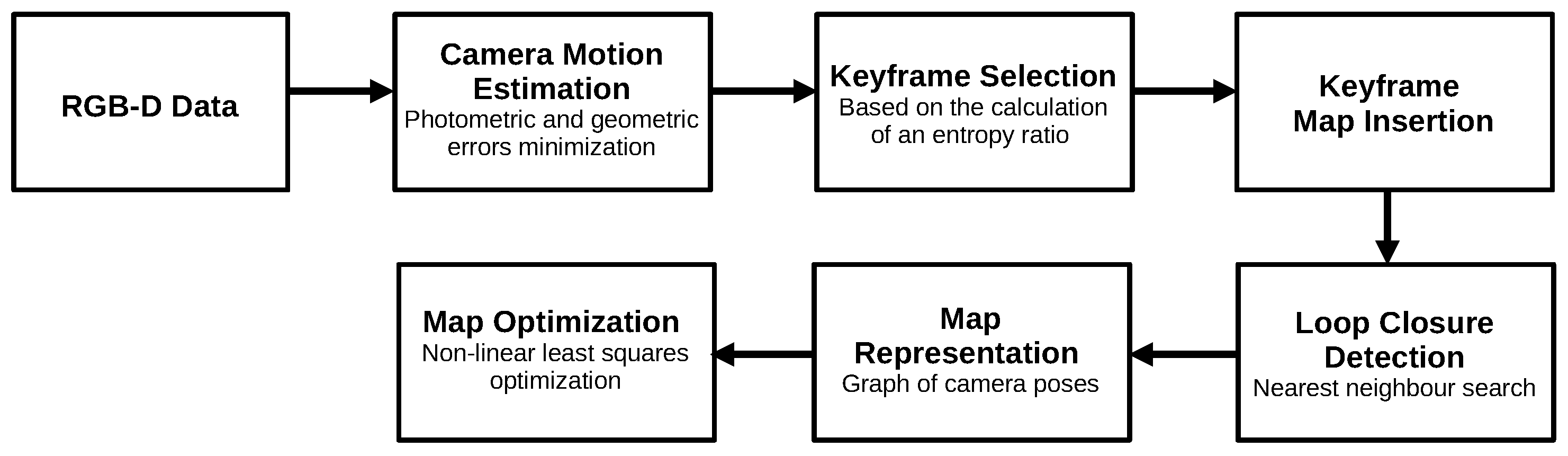
3.3.4. RGBDSLAMv2 (2014)

The RGBDSLAMv2 [96] is one of the most popular RGB-D-based algorithms and relies on feature extraction. It performs the RANSAC algorithm to estimate the transformation between the matched features and the ICP algorithm to obtain pose estimation. Finally, the system executes a global optimization and loop closure to eliminate the accumulated error. In addition, this method proposes using an environment measurement model (EMM) to validate the transformations obtained between the frames. The algorithm is based on SIFT features, which degrades its real-time performance. RGBDSLAMv2 presents a high computation consumption and requires a slow movement by the sensor for its correct operation [91]. Figure 23 represents the algorithm.

3.3.5. General Comments

Section 3.3 individually presented the most representative RGB-D-based techniques. Table 3 summarizes the main characteristics and analyzed criteria for the presented algorithms.
RGB-D-based SLAM algorithms represent an alternative solution to the visual-only and visual-inertial SLAM. In general, they construct dense maps, enabling them to represent the environment in greater detail. In addition, it is a more robust approach regarding low-texture environments thanks to the depth sensor. Concerning embedded implementations, it is possible to find, in the literature, several solutions searching to accelerate parts of the RGB-D-based algorithms that usually require more computation load, such as the ICP algorithm. Beshaw et al. [100] and Williams et al. [101] propose different architectures to accelerate the ICP algorithm, and Gautier et al. [102] implemented the ICP and the volumetric integration algorithms in a heterogeneous architecture. Recent publications have focused on developing robust RGB-D SLAM algorithms considering dynamic environments conditions [103,104,105].

4. Open Problems and Future Directions

Although the SLAM domain has been widely studied for years, there are still several open problems. The current state of the art of SLAM and odometry algorithms increasingly seeks to reinforce the algorithm’s robustness, optimize computational resources usage, and evolve the environment’s understanding in the map representations [8]. Concerning the robustness, SLAM and odometry techniques still present some major issues that undermine algorithms’ robustness [8]. One of them is the tracking failure [106]; facing some challenges or long-term scenarios, the algorithms may still fail to recognize and associate features in the current received image, resulting in inaccurate pose estimation. This may have consequences in loop closure techniques [107] and relocalizations [8,108]. As a solution to this issue, authors have been exploring new methods to deal with the SLAM problem. Recent works propose the incorporation of deep learning and spectral techniques [109,110] to increase the system’s robustness; some main examples the deep-learning-based algorithms are discussed in Section 4.1.
Another main issue that decreases the SLAM algorithms’ robustness is the assumption of static scenarios, while the real world presents dynamic environments; this may cause failures in tracking [111] and reconstruction [112]. Dealing with dynamic scenes may be considered a challenge, since it requires the algorithm to detect the dynamic object, avoid the tracking of the object, and exclude it from the map [113]. As mentioned in Section 3.3.5, several works have been published proposing solutions to this central issue; more representative examples are discussed in Section 4.3.
Besides the robustness, recent SLAM algorithms seek to consider the usage of the computational resources [8]. This current topic leads to the open problem of memory usage by map storage [8]. Storing the map in a long-term operation may considerably increase the memory usage, which may have consequences for memory-limited systems operation, e.g., embedded SLAM. However, it is already possible to find, in the literature, works proposing solutions for this topic. One example is the work of Opdenbosch et al. [114], who proposes an efficient map compression, and demonstrates its ability to significantly reduce the map’s data and size without losing relevant information. In addition to map storage, another major issue that influences resource usage is map sparsity. Dense and semi-dense maps provide a more detailed representation of the environment, but this feature has consequences for resource usage. It has already been demonstrated that sparse maps present lower power consumption compared to semi-dense and dense ones—Wan et al. [115]. Consequently, they may be more suitable for an embedded implementation, although they provide fewer details.
Currently, the SLAM algorithms also seek to evolve our understanding of the environment in the performed reconstructions [8]. Besides obtaining the geometric information, the algorithms obtain information about the environment by recognizing objects within it, for example. An evolving SLAM category that enables this better environment abstraction is the semantic-based SLAM. The semantic SLAM is a trending topic on SLAM, and some main examples are discussed in Section 4.2. Following this, we briefly discuss some recent and relevant articles that we believe are representatives as future directions of the visual-SLAM and visual-odometry fields.

4.1. Deep Learning-Based Algorithms

One remarkable algorithm that incorporates deep learning concepts is the UnDeepVO [116]. This monocular visual-odometry algorithm can perform pose and depth estimation via a deep neural network. The authors train UnDeepVO with unsupervised learning using stereo images; additionally, they consider both spatial and temporal dense information in the loss function of the training. This method proved to be more accurate and robust than other monocular methods, such as the ORB-SLAM (without loop closure). Recently, the same research group proposed the DeepSLAM [117]. The system considers a tracking-net and mapping-net trained using unsupervised learning, and considering spatial and temporal geometry in the loss function. The algorithm also contains a Loop-Net to perform loop detection. DeepSLAM presented a better performance than other monocular algorithms, as the ORB-SLAM, and better robustness than ORB-SLAM and LSD-SLAM.
Another relevant algorithm based on deep learning is the DF-SLAM [118]. DF-SLAM follows a framework similar to ORB-SLAM, but instead of using the hand-made features, explained in Section 2.1.1, it uses deep local features described by the TFeat network. The authors provide several results comparing DF-SLAM to ORB-SLAM2; for most sequences, the proposed algorithm obtained a better performance. Recently, it is possible to find, in the literature, several overviews [119,120,121] that address deep learning-based algorithms applied to depth estimation and the main concepts of SLAM’s direction. More methods that use deep learning techniques are discussed in Section 4.3 as a solution to dynamic SLAM algorithms.

4.2. Semantic-Based Algorithms

Incorporating semantic information on the visual-SLAM problem is a growing field, and has been attracting more attention in recent years. One important and recent study in this area is presented in [122]. The authors propose a new methodology for data association that incorporates information from an object detector, proposing a solution that can represent both data association and landmark class in a factor graph solution. This method presents reduced errors compared to other solutions incorporating semantic data association techniques. More methods containing semantic data are discussed in Section 4.3 as a solution to dynamic SLAM algorithms. As this field grows, it is also necessary to establish methods to validate the semantic-based algorithms. Authors in [123] introduce a new synthetically generated benchmark dataset that, besides the traditional ground truth of the trajectory, contains semantic labels, information about the scene composition, ground truth 3D models, and the pose of the objects. In addition, they propose evaluation metrics that may assess the semantic-based algorithms’ performance.

4.3. Dynamic SLAM Algorithms

Research studies into the SLAM algorithms considering dynamic environments are essential to increase the algorithms’ robustness to more realistic situations. Firstly, in [124], then in [125], Sun et al. propose a motion removal technique to deal with the environment’s dynamicity in RGB-D approach. In [125], the removal algorithm may be divided into two parts; first, it identifies the moving object and updates the foreground model using the error caused by the object in the image. Then, it performs the foreground segmentation. The algorithm obtained better performance, especially in high-dynamics environments, than some state-of-the-art techniques, such as DVO.
An essential algorithm robust to dynamic scenes is the Dynamic-SLAM proposed by Xiao et al. [126]; this method incorporates both deep learning and semantic techniques. The system employs a CNN to detect dynamic objects at a semantic level; it separates the dynamics and statics features, considering the dynamic ones as outliers. In addition, they propose a compensation algorithm to increase the detection accuracy and a feature-based framework. The tracking thread incorporates the semantic data, discarding or reserving the features. Dynamic-SLAM presented a greater accuracy than other methods such as LSD-SLAM, SVO, and PTAM; and better robustness compared to ORB-SLAM2.
DynaSLAM II [127] is another relevant method that incorporates semantic segmentation to track dynamic objects. This algorithm is based on ORB-SLAM2 and performs semantic segmentation and feature extraction at each new frame. This algorithm does not make assumptions about the dynamic objects and performs the data association of dynamic and static features. Static features are used to estimate the initial camera poses, and then trajectories, bounding boxes, and 3D points are optimized. DynaSLAMII showed to present a performance comparable to other state-of-the-art algorithms, such as the ORB-SLAM2.

5. Datasets and Benchmarking

Among all the SLAM algorithms in the literature, it is essential to achieve a fair comparison between them to determine which one presents a better performance in certain situations. Several benchmarking datasets with different characteristics are proposed in the literature to explore the SLAM capabilities and robustness. Here, we present the publicly available benchmark dataset used to evaluate the presented SLAM algorithms in their original articles.
The TUM RGB-D dataset [128] consists of several image sequences containing color and depth images recorded in indoor environments with a Microsoft Kinetic in two different platforms: robot and handheld. The system was synchronized with a motion-capture system to provide the ground truth. In addition, the authors propose two metrics to evaluate the local accuracy and the global consistency of the trajectory; they are relative pose error and absolute trajectory error, respectively. The KITTI dataset [129] contains outdoor sequences recorded by color and grayscale stereo cameras. The KITTI also present data from a 3D laser scanner and the ground truth provided by an INS/GPS. The sensor system is synchronized and mounted on a car. In addition, the authors provide tracklets for a dynamic objects classification and benchmarks to evaluate robotics tasks, such as visual odometry and SLAM.
Another main benchmark dataset is the ICL-NUIM [130]. The dataset focuses on RGB-D algorithms and provides data for the evaluation of the 3D reconstruction through eight synthetically generated indoor scenes. A handheld RGB-D camera generates the sequences, and the ground truth consists of a 3D surface model and the estimated trajectory by a SLAM algorithm [131]. The EuRoC benchmark dataset [23] is widely used to evaluate visual-only and visual-inertial SLAM and odometry algorithms. The data were collected in two indoor environments by a micro aerial vehicle (MAV), and it provides eleven sequences of stereo images and IMU data. The ground truth is obtained by a total station and a motion capture system.
A dataset commonly used to evaluate monocular systems is the TUM MonoVO [30]. It contains several photometrically calibrated indoor and outdoor sequences provided by two handheld non-stereo monocular cameras. Due to the variety of the scenes, the authors do not provide a ground-truth from the poses, but they perform large sequences that start and end at the same position, allowing the evaluation of the loop drifts. Lastly, a dataset provided for visual-inertial systems evaluation is the TUM VI dataset [132]. It provides several indoor and outdoor sequences captured by a stereo camera synchronized with an IMU. The sensor system is handheld, and, as for the TUM MonoVO, it was impossible to establish the ground truth for the entire sequences. However, they provide the ground truth via a motion capture system for the beginning and end of the system.
Table 4 summarizes the main benchmark datasets characteristics presented in this work.

6. Conclusions

The visual-based SLAM techniques represent a wide field of research thanks to their robustness and accuracy provided by a cheap and small sensor system. The literature presents many different visual-SLAM algorithms that make researchers’ choices difficult, without criteria, when it comes to evaluating their benefits and drawbacks. In this paper, we introduced the main visual-based SLAM approaches and a brief description and systematic analyses of a set of the most exemplary techniques of each approach. To guide the choices among all the algorithms, we proposed six criteria that are limiting factors to several SLAM projects: the algorithm type, the density of the reconstructed map, the presence of global optimizations and loop closures techniques, its availability, and the embedded implementations already performed. Researchers can consider each criterion according to their application, and obtain an initial analysis from the presented paper. In addition, we presented some major issues, suggested future directions for the field, and discussed the main benchmarking datasets for visual-SLAM and odometry algorithms evaluation. Regarding future works, we will apply the proposed criteria analysis to nuclear decommissioning scenarios. The best SLAM algorithm shall be selected after considering the variety of features and specificities that this environment and application possess.

Author Contributions

Conceptualization, A.M.B., M.M., Y.M., G.C. and F.C.; methodology, A.M.B., M.M. and Y.M.; formal analysis, A.M.B., M.M., Y.M. and F.C.; investigation, A.M.B.; writing—original draft preparation, A.M.B.; writing—review and editing, M.M., Y.M., G.C. and F.C.; supervision, M.M., Y.M., G.C. and F.C. All authors have read and agreed to the published version of the manuscript.

Funding

This research received no external funding.

Institutional Review Board Statement

Not applicable.

Informed Consent Statement

Not applicable.

Conflicts of Interest

The authors declare no conflict of interest.

References

  1. Smith, R.; Cheeseman, P. On the Representation and Estimation of Spatial Uncertainty. Int. J. Robot. Res. 1987, 5, 56–68. [Google Scholar] [CrossRef]
  2. Jinyu, L.; Bangbang, Y.; Danpeng, C.; Nan, W.; Guofeng, Z.; Hujun, B. Survey and evaluation of monocular visual-inertial SLAM algorithms for augmented reality. Virtual Real. Intell. Hardw. 2019, 1, 386–410. [Google Scholar] [CrossRef]
  3. Covolan, J.P.; Sementille, A.; Sanches, S. A mapping of visual SLAM algorithms and their applications in augmented reality. In Proceedings of the 2020 22nd Symposium on Virtual and Augmented Reality (SVR), Porto de Galinhas, Brazil, 7–10 November 2020. [Google Scholar] [CrossRef]
  4. Singandhupe, A.; La, H. A Review of SLAM Techniques and Security in Autonomous Driving. In Proceedings of the 2019 Third IEEE International Conference on Robotic Computing (IRC), Naples, Italy, 25–27 February 2019; pp. 602–607. [Google Scholar] [CrossRef]
  5. Dworakowski, D.; Thompson, C.; Pham-Hung, M.; Nejat, G. A Robot Architecture Using ContextSLAM to Find Products in Unknown Crowded Retail Environments. Robotics 2021, 10, 110. [Google Scholar] [CrossRef]
  6. Ruan, K.; Wu, Z.; Xu, Q. Smart Cleaner: A New Autonomous Indoor Disinfection Robot for Combating the COVID-19 Pandemic. Robotics 2021, 10, 87. [Google Scholar] [CrossRef]
  7. Liu, C.; Zhou, C.; Cao, W.; Li, F.; Jia, P. A Novel Design and Implementation of Autonomous Robotic Car Based on ROS in Indoor Scenario. Robotics 2020, 9, 19. [Google Scholar] [CrossRef] [Green Version]
  8. Cadena, C.; Carlone, L.; Carrillo, H.; Latif, Y.; Scaramuzza, D.; Neira, J.; Reid, I.; Leonard, J.J. Past, Present, and Future of Simultaneous Localization and Mapping: Toward the Robust-Perception Age. IEEE Trans. Robot. 2016, 32, 1309–1332. [Google Scholar] [CrossRef] [Green Version]
  9. Stachniss, C. Robotic Mapping and Exploration; Springer: Berlin/Heidelberg, Germany, 2009; Volume 55. [Google Scholar]
  10. Taketomi, T.; Uchiyama, H.; Ikeda, S. Visual SLAM algorithms: A survey from 2010 to 2016. IPSJ Trans. Comput. Vis. Appl. 2017, 9, 1–11. [Google Scholar] [CrossRef]
  11. Kabzan, J.; Valls, M.; Reijgwart, V.; Hendrikx, H.; Ehmke, C.; Prajapat, M.; Bühler, A.; Gosala, N.; Gupta, M.; Sivanesan, R.; et al. AMZ Driverless: The Full Autonomous Racing System. J. Field Robot. 2020, 37, 1267–1294. [Google Scholar] [CrossRef]
  12. Durrant-Whyte, H.; Bailey, T. Simultaneous localization and mapping: Part I. IEEE Robot. Autom. Mag. 2006, 13, 99–110. [Google Scholar] [CrossRef] [Green Version]
  13. Bailey, T.; Durrant-Whyte, H. Simultaneous localization and mapping (SLAM): Part II. IEEE Robot. Autom. Mag. 2006, 13, 108–117. [Google Scholar] [CrossRef] [Green Version]
  14. Yousif, K.; Bab-Hadiashar, A.; Hoseinnezhad, R. An Overview to Visual Odometry and Visual SLAM: Applications to Mobile Robotics. Intell. Ind. Syst. 2015, 1, 289–311. [Google Scholar] [CrossRef]
  15. Fuentes-Pacheco, J.; Ruiz-Ascencio, J.; Rendón-Mancha, J.M. Visual simultaneous localization and mapping: A survey. Artif. Intell. Rev. 2015, 43, 55–81. [Google Scholar] [CrossRef]
  16. Servières, M.; Renaudin, V.; Dupuis, A.; Antigny, N. Visual and Visual-Inertial SLAM: State of the Art, Classification, and Experimental Benchmarking. J. Sensors 2021, 2021, 2054828. [Google Scholar] [CrossRef]
  17. Gui, J.; Gu, D.; Wang, S.; Hu, H. A review of visual inertial odometry from filtering and optimisation perspectives. Adv. Robot. 2015, 29, 1–13. [Google Scholar] [CrossRef]
  18. Chen, C.; Zhu, H.; Li, M.; You, S. A Review of Visual-Inertial Simultaneous Localization and Mapping from Filtering-Based and Optimization-Based Perspectives. Robotics 2018, 7, 45. [Google Scholar] [CrossRef] [Green Version]
  19. Huang, G. Visual-Inertial Navigation: A Concise Review. In Proceedings of the 2019 International Conference on Robotics and Automation (ICRA), Montreal, QC, Canada, 20–24 May 2019; pp. 9572–9582. [Google Scholar] [CrossRef] [Green Version]
  20. Chen, K.; Lai, Y.; Hu, S. 3D indoor scene modeling from RGB-D data: A survey. Comput. Vis. Media 2015, 1, 267–278. [Google Scholar] [CrossRef] [Green Version]
  21. Zhang, S.; Zheng, L.; Tao, W. Survey and Evaluation of RGB-D SLAM. IEEE Access 2021, 9, 21367–21387. [Google Scholar] [CrossRef]
  22. Campos, C.; Elvira, R.; Rodríguez, J.J.G.; Montiel, J.M.M.; D. Tardós, J. ORB-SLAM3: An Accurate Open-Source Library for Visual, Visual–Inertial, and Multimap SLAM. IEEE Trans. Robot. 2021, 37, 1874–1890. [Google Scholar] [CrossRef]
  23. Burri, M.; Nikolic, J.; Gohl, P.; Schneider, T.; Rehder, J.; Omari, S.; Achtelik, M.; Siegwart, R. The EuRoC micro aerial vehicle datasets. Int. J. Robot. Res. 2016, 35, 1157–1163. [Google Scholar] [CrossRef]
  24. Engel, J.; Schöps, T.; Cremers, D. LSD-SLAM: Large-Scale Direct Monocular SLAM. In Computer Vision–ECCV 2014; Fleet, D., Pajdla, T., Schiele, B., Tuytelaars, T., Eds.; Springer International Publishing: Cham, Switzerland, 2014; pp. 834–849. [Google Scholar]
  25. Bianco, S.; Ciocca, G.; Marelli, D. Evaluating the Performance of Structure from Motion Pipelines. J. Imaging 2018, 4, 98. [Google Scholar] [CrossRef] [Green Version]
  26. Lepetit, V.; Moreno-Noguer, F.; Fua, P. EPnP: An Accurate O(n) Solution to the PnP Problem. Int. J. Comput. Vis. 2008, 81, 155. [Google Scholar] [CrossRef] [Green Version]
  27. Davison, A.J.; Reid, I.D.; Molton, N.D.; Stasse, O. MonoSLAM: Real-Time Single Camera SLAM. IEEE Trans. Pattern Anal. Mach. Intell. 2007, 29, 1052–1067. [Google Scholar] [CrossRef] [PubMed] [Green Version]
  28. Loo, S.Y.; Amiri, A.; Mashohor, S.; Tang, S.; Zhang, H. CNN-SVO: Improving the Mapping in Semi-Direct Visual Odometry Using Single-Image Depth Prediction. In Proceedings of the 2019 International Conference on Robotics and Automation (ICRA), Montreal, QC, Canada, 20–24 May 2019. [Google Scholar]
  29. Boikos, K.; Bouganis, C.S. Semi-dense SLAM on an FPGA SoC. In Proceedings of the 2016 26th International Conference on Field Programmable Logic and Applications (FPL), Lausanne, Switzerland, 29 August–2 September 2016; pp. 1–4. [Google Scholar] [CrossRef] [Green Version]
  30. Engel, J.; Usenko, V.; Cremers, D. A Photometrically Calibrated Benchmark For Monocular Visual Odometry. arXiv 2016, arXiv:1607.02555. [Google Scholar]
  31. Engel, J.; Koltun, V.; Cremers, D. Direct Sparse Odometry. IEEE Trans. Pattern Anal. Mach. Intell. 2018, 40, 611–625. [Google Scholar] [CrossRef] [PubMed]
  32. Canovas, B.; Rombaut, M.; Nègre, A.; Pellerin, D.; Olympieff, S. Speed and Memory Efficient Dense RGB-D SLAM in Dynamic Scenes. In Proceedings of the IROS 2020—IEEE/RSJ International Conference on Intelligent Robots and Systems, Las Vegas, NV, USA, 25–29 October 2020; pp. 4996–5001. [Google Scholar] [CrossRef]
  33. Bresson, G.; Alsayed, Z.; Yu, L.; Glaser, S. Simultaneous Localization and Mapping: A Survey of Current Trends in Autonomous Driving. IEEE Trans. Intell. Veh. 2017, 2, 194–220. [Google Scholar] [CrossRef] [Green Version]
  34. Vincke, B.; Elouardi, A.; Lambert, A. Design and evaluation of an embedded system based SLAM applications. In Proceedings of the 2010 IEEE/SICE International Symposium on System Integration, Sendai, Japan, 21–22 December 2010; pp. 224–229. [Google Scholar] [CrossRef]
  35. Vincke, B.; Elouardi, A.; Lambert, A.; Merigot, A. Efficient implementation of EKF-SLAM on a multi-core embedded system. In Proceedings of the IECON 2012—38th Annual Conference on IEEE Industrial Electronics Society, Montreal, QC, Canada, 25–28 October 2012; pp. 3049–3054. [Google Scholar] [CrossRef]
  36. Klein, G.; Murray, D. Parallel Tracking and Mapping for Small AR Workspaces. In Proceedings of the 2007 6th IEEE and ACM International Symposium on Mixed and Augmented Reality, Nara, Japan, 13–16 November 2007; pp. 225–234. [Google Scholar] [CrossRef]
  37. Serrata, A.A.J.; Yang, S.; Li, R. An intelligible implementation of FastSLAM2.0 on a low-power embedded architecture. EURASIP J. Embed. Syst. 2017, 2017, 27. [Google Scholar]
  38. Newcombe, R.A.; Lovegrove, S.J.; Davison, A.J. DTAM: Dense tracking and mapping in real-time. In Proceedings of the 2011 International Conference on Computer Vision, Barcelona, Spain, 6–13 November 2011; pp. 2320–2327. [Google Scholar]
  39. Ondrúška, P.; Kohli, P.; Izadi, S. MobileFusion: Real-Time Volumetric Surface Reconstruction and Dense Tracking on Mobile Phones. IEEE Trans. Vis. Comput. Graph. 2015, 21, 1251–1258. [Google Scholar] [CrossRef]
  40. Forster, C.; Pizzoli, M.; Scaramuzza, D. SVO: Fast semi-direct monocular visual odometry. In Proceedings of the 2014 IEEE International Conference on Robotics and Automation (ICRA), Hong Kong, China, 31 May–7 June 2014; pp. 15–22. [Google Scholar] [CrossRef] [Green Version]
  41. Mur-Artal, R.; Montiel, J.; Tardos, J. ORB-SLAM: A versatile and accurate monocular SLAM system. IEEE Trans. Robot. 2015, 31, 1147–1163. [Google Scholar] [CrossRef] [Green Version]
  42. Forster, C.; Zhang, Z.; Gassner, M.; Werlberger, M.; Scaramuzza, D. SVO: Semidirect Visual Odometry for Monocular and Multicamera Systems. IEEE Trans. Robot. 2017, 33, 249–265. [Google Scholar] [CrossRef] [Green Version]
  43. Boikos, K.; Bouganis, C.S. A high-performance system-on-chip architecture for direct tracking for SLAM. In Proceedings of the 2017 27th International Conference on Field Programmable Logic and Applications (FPL), Gent, Belgium, 4–6 September 2017; pp. 1–7. [Google Scholar] [CrossRef] [Green Version]
  44. Mur-Artal, R.; Tardós, J.D. ORB-SLAM2: An Open-Source SLAM System for Monocular, Stereo, and RGB-D Cameras. IEEE Trans. Robot. 2017, 33, 1255–1262. [Google Scholar] [CrossRef] [Green Version]
  45. Zhan, Z.; Jian, W.; Li, Y.; Yue, Y. A SLAM Map Restoration Algorithm Based on Submaps and an Undirected Connected Graph. IEEE Access 2021, 9, 12657–12674. [Google Scholar] [CrossRef]
  46. Abouzahir, M.; Elouardi, A.; Latif, R.; Bouaziz, S.; Tajer, A. Embedding SLAM algorithms: Has it come of age? Robot. Auton. Syst. 2018, 100, 14–26. [Google Scholar] [CrossRef]
  47. Yu, J.; Gao, F.; Cao, J.; Yu, C.; Zhang, Z.; Huang, Z.; Wang, Y.; Yang, H. CNN-based Monocular Decentralized SLAM on embedded FPGA. In Proceedings of the 2020 IEEE International Parallel and Distributed Processing Symposium Workshops (IPDPSW), New Orleans, LA, USA, 18–22 May 2020; pp. 66–73. [Google Scholar] [CrossRef]
  48. Tateno, K.; Tombari, F.; Laina, I.; Navab, N. CNN-SLAM: Real-Time Dense Monocular SLAM with Learned Depth Prediction. In Proceedings of the 2017 IEEE Conference on Computer Vision and Pattern Recognition (CVPR), Honolulu, HI, USA, 21–26 July 2017; pp. 6565–6574. [Google Scholar] [CrossRef] [Green Version]
  49. Gao, X.; Wang, R.; Demmel, N.; Cremers, D. LDSO: Direct Sparse Odometry with Loop Closure. In Proceedings of the 2018 IEEE/RSJ International Conference on Intelligent Robots and Systems (IROS), Madrid, Spain, 1–5 October 2018. [Google Scholar]
  50. Davison, A.J. SceneLib 1.0. 2006. Available online: https://www.doc.ic.ac.uk/~ajd/Scene/index.html (accessed on 21 January 2022).
  51. Klein, G.; Murray, D. Parallel Tracking and Mapping on a camera phone. In Proceedings of the 2009 8th IEEE International Symposium on Mixed and Augmented Reality, Orlando, FL, USA, 19–22 October 2009; pp. 83–86. [Google Scholar]
  52. Oxford-PTAM. Available online: https://github.com/Oxford-PTAM/PTAM-GPL (accessed on 21 January 2022).
  53. OpenDTAM. Available online: https://github.com/anuranbaka/OpenDTAM (accessed on 21 January 2022).
  54. SVO. Available online: https://github.com/uzh-rpg/rpg_svo (accessed on 21 January 2022).
  55. LSD-SLAM: Large-Scale Direct Monocular SLAM. Available online: https://github.com/tum-vision/lsd_slam (accessed on 21 January 2022).
  56. ORB-SLAM2. Available online: https://github.com/raulmur/ORB_SLAM2 (accessed on 21 January 2022).
  57. CNN SLAM. Available online: https://github.com/iitmcvg/CNN_SLAM (accessed on 21 January 2022).
  58. DSO: Direct Sparse Odometry. Available online: https://github.com/JakobEngel/dso (accessed on 21 January 2022).
  59. Piat, J.; Fillatreau, P.; Tortei, D.; Brenot, F.; Devy, M. HW/SW co-design of a visual SLAM application. J.-Real-Time Image Process. 2018. [Google Scholar] [CrossRef] [Green Version]
  60. DPU for Convolutional Neural Network. Available online: https://www.xilinx.com/products/intellectual-property/dpu.html#overview (accessed on 21 January 2022).
  61. Xu, Z.; Yu, J.; Yu, C.; Shen, H.; Wang, Y.; Yang, H. CNN-based Feature-point Extraction for Real-time Visual SLAM on Embedded FPGA. In Proceedings of the 2020 IEEE 28th Annual International Symposium on Field-Programmable Custom Computing Machines (FCCM), Fayetteville, AR, USA, 3–6 May 2020; pp. 33–37. [Google Scholar]
  62. Mourikis, A.I.; Roumeliotis, S.I. A Multi-State Constraint Kalman Filter for Vision-aided Inertial Navigation. In Proceedings of the 2007 IEEE International Conference on Robotics and Automation, Roma, Italy, 10–14 April 2007; pp. 3565–3572. [Google Scholar]
  63. Sun, K.; Mohta, K.; Pfrommer, B.; Watterson, M.; Liu, S.; Mulgaonkar, Y.; Taylor, C.J.; Kumar, V. Robust Stereo Visual Inertial Odometry for Fast Autonomous Flight. IEEE Robot. Autom. Lett. 2018, 3, 965–972. [Google Scholar] [CrossRef] [Green Version]
  64. Li, S.P.; Zhang, T.; Gao, X.; Wang, D.; Xian, Y. Semi-direct monocular visual and visual-inertial SLAM with loop closure detection. Robot. Auton. Syst. 2019, 112, 201–210. [Google Scholar] [CrossRef]
  65. Delmerico, J.; Scaramuzza, D. A Benchmark Comparison of Monocular Visual-Inertial Odometry Algorithms for Flying Robots. In Proceedings of the 2018 IEEE International Conference on Robotics and Automation (ICRA), Brisbane, Australia, 21–25 May 2018; pp. 2502–2509. [Google Scholar] [CrossRef]
  66. Li, M.; Mourikis, A.I. Improving the accuracy of EKF-based visual-inertial odometry. In Proceedings of the 2012 IEEE International Conference on Robotics and Automation, Saint Paul, MI, USA, 14–18 May 2012; pp. 828–835. [Google Scholar]
  67. Leutenegger, S.; Lynen, S.; Bosse, M.; Siegwart, R.; Furgale, P. Keyframe-Based Visual-Inertial Odometry Using Nonlinear Optimization. Int. J. Robot. Res. 2014, 34, 314–334. [Google Scholar] [CrossRef] [Green Version]
  68. Nikolic, J.; Rehder, J.; Burri, M.; Gohl, P.; Leutenegger, S.; Furgale, P.T.; Siegwart, R. A synchronized visual-inertial sensor system with FPGA pre-processing for accurate real-time SLAM. In Proceedings of the 2014 IEEE International Conference on Robotics and Automation (ICRA), Hong Kong, China, 31 May–7 June 2014; pp. 431–437. [Google Scholar] [CrossRef] [Green Version]
  69. Bloesch, M.; Omari, S.; Hutter, M.; Siegwart, R. Robust visual inertial odometry using a direct EKF-based approach. In Proceedings of the 2015 IEEE/RSJ International Conference on Intelligent Robots and Systems (IROS), Hamburg, Germany, 28 September–3 October 2015; pp. 298–304. [Google Scholar] [CrossRef] [Green Version]
  70. Von Stumberg, L.; Usenko, V.; Cremers, D. Direct Sparse Visual-Inertial Odometry Using Dynamic Marginalization. In Proceedings of the 2018 IEEE International Conference on Robotics and Automation (ICRA), Brisbane, Australia, 21–25 May 2018; pp. 2510–2517. [Google Scholar] [CrossRef] [Green Version]
  71. Mur-Artal, R.; Tardós, J.D. Visual-Inertial Monocular SLAM With Map Reuse. IEEE Robot. Autom. Lett. 2017, 2, 796–803. [Google Scholar] [CrossRef] [Green Version]
  72. Silveira, O.C.B.; de Melo, J.G.O.C.; Moreira, L.A.S.; Pinto, J.B.N.G.; Rodrigues, L.R.L.; Rosa, P.F.F. Evaluating a Visual Simultaneous Localization and Mapping Solution on Embedded Platforms. In Proceedings of the 2020 IEEE 29th International Symposium on Industrial Electronics (ISIE), Delft, The Netherlands, 17–19 June 2020; pp. 530–535. [Google Scholar] [CrossRef]
  73. Qin, T.; Li, P.; Shen, S. VINS-Mono: A Robust and Versatile Monocular Visual-Inertial State Estimator. IEEE Trans. Robot. 2018, 34, 1004–1020. [Google Scholar] [CrossRef] [Green Version]
  74. Paul, M.K.; Wu, K.; Hesch, J.A.; Nerurkar, E.D.; Roumeliotis, S.I. A comparative analysis of tightly-coupled monocular, binocular, and stereo VINS. In Proceedings of the 2017 IEEE International Conference on Robotics and Automation (ICRA), Singapore, 29 May–3 June 2017; pp. 165–172. [Google Scholar] [CrossRef]
  75. Campos, C.; Montiel, J.M.; Tardós, J.D. Inertial-Only Optimization for Visual-Inertial Initialization. In Proceedings of the 2020 IEEE International Conference on Robotics and Automation (ICRA), Paris, France, 31 May–31 August 2020; pp. 51–57. [Google Scholar] [CrossRef]
  76. Seiskari, O.; Rantalankila, P.; Kannala, J.; Ylilammi, J.; Rahtu, E.; Solin, A. HybVIO: Pushing the Limits of Real-Time Visual-Inertial Odometry. In Proceedings of the IEEE/CVF Winter Conference on Applications of Computer Vision (WACV), Waikoloa, HI, USA, 4–8 January 2022; pp. 701–710. [Google Scholar]
  77. Merzlyakov, A.; Macenski, S. A Comparison of Modern General-Purpose Visual SLAM Approaches. In Proceedings of the 2021 IEEE/RSJ International Conference on Intelligent Robots and Systems (IROS), Prague, Czech Republic, 27 September–1 October 2021; pp. 9190–9197. [Google Scholar] [CrossRef]
  78. dvo. Available online: https://github.com/daniilidis-group/msckf_mono (accessed on 21 January 2022).
  79. msckf_vio. Available online: https://github.com/KumarRobotics/msckf_vio (accessed on 21 January 2022).
  80. OKVIS. Available online: https://github.com/ethz-asl/okvis (accessed on 21 January 2022).
  81. ROVIO. Available online: https://github.com/ethz-asl/rovio (accessed on 21 January 2022).
  82. VINS-Mono. Available online: https://github.com/HKUST-Aerial-Robotics/VINS-Mono (accessed on 21 January 2022).
  83. VI-Stereo-DSO. Available online: https://github.com/RonaldSun/VI-Stereo-DSO (accessed on 21 January 2022).
  84. ORB-SLAM3: An Accurate Open-Source Library for Visual, Visual-Inertial and Multi-Map SLAM. Available online: https://github.com/UZ-SLAMLab/ORB_SLAM3 (accessed on 21 January 2022).
  85. Aslam, M.S.; Aziz, M.I.; Naveed, K.; uz Zaman, U.K. An RPLiDAR based SLAM equipped with IMU for Autonomous Navigation of Wheeled Mobile Robot. In Proceedings of the 2020 IEEE 23rd International Multitopic Conference (INMIC), Bahawalpur, Pakistan, 5–7 November 2020; pp. 1–5. [Google Scholar] [CrossRef]
  86. Nguyen, T.M.; Yuan, S.; Cao, M.; Nguyen, T.H.; Xie, L. VIRAL SLAM: Tightly Coupled Camera-IMU-UWB-Lidar SLAM. arXiv 2021, arXiv:2105.03296. [Google Scholar]
  87. Chang, L.; Niu, X.; Liu, T. GNSS/IMU/ODO/LiDAR-SLAM Integrated Navigation System Using IMU/ODO Pre-Integration. Sensors 2020, 20, 4702. [Google Scholar] [CrossRef]
  88. Zuñiga-Noël, D.; Moreno, F.A.; Gonzalez-Jimenez, J. An Analytical Solution to the IMU Initialization Problem for Visual-Inertial Systems. IEEE Robot. Autom. Lett. 2021, 6, 6116–6122. [Google Scholar] [CrossRef]
  89. Petit, B.; Guillemard, R.; Gay-Bellile, V. Time Shifted IMU Preintegration for Temporal Calibration in Incremental Visual-Inertial Initialization. In Proceedings of the 2020 International Conference on 3D Vision (3DV), Fukuoka, Japan, 25–28 November 2020; pp. 171–179. [Google Scholar] [CrossRef]
  90. Newcombe, R.A.; Izadi, S.; Hilliges, O.; Molyneaux, D.; Kim, D.; Davison, A.J.; Kohi, P.; Shotton, J.; Hodges, S.; Fitzgibbon, A. KinectFusion: Real-time dense surface mapping and tracking. In Proceedings of the 2011 10th IEEE International Symposium on Mixed and Augmented Reality, Basel, Switzerland, 26–29 October 2011; pp. 127–136. [Google Scholar]
  91. Jin, Q.; Liu, Y.; Man, Y.; Li, F. Visual SLAM with RGB-D Cameras. In Proceedings of the 2019 Chinese Control Conference (CCC), Guangzhou, China, 27–30 July 2019; pp. 4072–4077. [Google Scholar] [CrossRef]
  92. Nardi, L.; Bodin, B.; Zia, M.Z.; Mawer, J.; Nisbet, A.; Kelly, P.H.J.; Davison, A.J.; Luján, M.; O’Boyle, M.F.P.; Riley, G.D.; et al. Introducing SLAMBench, a performance and accuracy benchmarking methodology for SLAM. In Proceedings of the 2015 IEEE International Conference on Robotics and Automation (ICRA), Seattle, WA, USA, 26–30 May 2015; pp. 5783–5790. [Google Scholar]
  93. Bodin, B.; Nardi, L.; Zia, M.Z.; Wagstaff, H.; Shenoy, G.S.; Emani, M.; Mawer, J.; Kotselidis, C.; Nisbet, A.; Lujan, M.; et al. Integrating algorithmic parameters into benchmarking and design space exploration in 3D scene understanding. In Proceedings of the 2016 International Conference on Parallel Architecture and Compilation Techniques (PACT), Haifa, Israel, 11–15 September 2016; pp. 57–69. [Google Scholar] [CrossRef] [Green Version]
  94. Salas-Moreno, R.F.; Newcombe, R.A.; Strasdat, H.; Kelly, P.H.; Davison, A.J. SLAM++: Simultaneous Localisation and Mapping at the Level of Objects. In Proceedings of the 2013 IEEE Conference on Computer Vision and Pattern Recognition, Portland, OR, USA, 23–28 June 2013; pp. 1352–1359. [Google Scholar] [CrossRef] [Green Version]
  95. Kerl, C.; Sturm, J.; Cremers, D. Dense visual SLAM for RGB-D cameras. In Proceedings of the 2013 IEEE/RSJ International Conference on Intelligent Robots and Systems, Tokyo, Japan, 3–7 November 2013; pp. 2100–2106. [Google Scholar]
  96. Endres, F.; Hess, J.; Sturm, J.; Cremers, D.; Burgard, W. 3-D Mapping With an RGB-D Camera. IEEE Trans. Robot. 2014, 30, 177–187. [Google Scholar] [CrossRef]
  97. KinectFusion. Available online: https://github.com/ParikaGoel/KinectFusion (accessed on 21 January 2022).
  98. rgbdslam. Available online: http://ros.org/wiki/rgbdslam (accessed on 21 January 2022).
  99. dvo. Available online: https://github.com/tum-vision/dvo (accessed on 21 January 2022).
  100. Belshaw, M.S.; Greenspan, M.A. A high speed iterative closest point tracker on an FPGA platform. In Proceedings of the 2009 IEEE 12th International Conference on Computer Vision Workshops, ICCV Workshops, Kyoto, Japan, 27 September–4 October 2009; pp. 1449–1456. [Google Scholar] [CrossRef] [Green Version]
  101. Williams, B. Evaluation of a SoC for Real-time 3D SLAM. Doctoral Dissertation, Iowa State University, Ames, IA, USA, 2017. [Google Scholar]
  102. Gautier, Q.; Shearer, A.; Matai, J.; Richmond, D.; Meng, P.; Kastner, R. Real-time 3D reconstruction for FPGAs: A case study for evaluating the performance, area, and programmability trade-offs of the Altera OpenCL SDK. In Proceedings of the 2014 International Conference on Field-Programmable Technology (FPT), Shanghai, China, 10–12 December 2014; pp. 326–329. [Google Scholar] [CrossRef]
  103. Zhang, T.; Zhang, H.; Li, Y.; Nakamura, Y.; Zhang, L. FlowFusion: Dynamic Dense RGB-D SLAM Based on Optical Flow. In Proceedings of the 2020 IEEE International Conference on Robotics and Automation (ICRA), Paris, France, 31 May–31 August 2020; pp. 7322–7328. [Google Scholar] [CrossRef]
  104. Dai, W.; Zhang, Y.; Li, P.; Fang, Z.; Scherer, S. RGB-D SLAM in Dynamic Environments Using Point Correlations. IEEE Trans. Pattern Anal. Mach. Intell. 2020, 44, 373–389. [Google Scholar] [CrossRef]
  105. Ai, Y.; Rui, T.; Lu, M.; Fu, L.; Liu, S.; Wang, S. DDL-SLAM: A Robust RGB-D SLAM in Dynamic Environments Combined With Deep Learning. IEEE Access 2020, 8, 162335–162342. [Google Scholar] [CrossRef]
  106. Deng, X.; Zhang, Z.; Sintov, A.; Huang, J.; Bretl, T. Feature-constrained Active Visual SLAM for Mobile Robot Navigation. In Proceedings of the 2018 IEEE International Conference on Robotics and Automation (ICRA), Brisbane, Australia, 21–25 May 2018; pp. 7233–7238. [Google Scholar] [CrossRef]
  107. Jaenal, A.; Zuñiga-Nöel, D.; Gomez-Ojeda, R.; Gonzalez-Jimenez, J. Improving Visual SLAM in Car-Navigated Urban Environments with Appearance Maps. In Proceedings of the 2020 IEEE/RSJ International Conference on Intelligent Robots and Systems (IROS), Las Vegas, NV, USA, 25–29 October 2020; pp. 4679–4685. [Google Scholar] [CrossRef]
  108. Li, D.; Shi, X.; Long, Q.; Liu, S.; Yang, W.; Wang, F.; Wei, Q.; Qiao, F. DXSLAM: A Robust and Efficient Visual SLAM System with Deep Features. In Proceedings of the 2020 IEEE/RSJ International Conference on Intelligent Robots and Systems (IROS), Las Vegas, NV, USA, 25–29 October 2020; pp. 4958–4965. [Google Scholar] [CrossRef]
  109. Xu, Q.; Kuang, H.; Kneip, L.; Schwertfeger, S. Rethinking the Fourier-Mellin Transform: Multiple Depths in the Camera’s View. Remote Sens. 2021, 13, 1000. [Google Scholar] [CrossRef]
  110. Xu, Q.; Chavez, A.G.; Bülow, H.; Birk, A.; Schwertfeger, S. Improved Fourier Mellin Invariant for Robust Rotation Estimation with Omni-Cameras. In Proceedings of the 2019 IEEE International Conference on Image Processing (ICIP), Taipei, Taiwan, 22–25 September 2019; pp. 320–324. [Google Scholar] [CrossRef] [Green Version]
  111. Scona, R.; Jaimez, M.; Petillot, Y.R.; Fallon, M.; Cremers, D. StaticFusion: Background Reconstruction for Dense RGB-D SLAM in Dynamic Environments. In Proceedings of the 2018 IEEE International Conference on Robotics and Automation (ICRA), Brisbane, Australia, 21–25 May 2018; pp. 3849–3856. [Google Scholar] [CrossRef]
  112. Soares, J.C.V.; Gattass, M.; Meggiolaro, M.A. Visual SLAM in Human Populated Environments: Exploring the Trade-off between Accuracy and Speed of YOLO and Mask R-CNN. In Proceedings of the 2019 19th International Conference on Advanced Robotics (ICAR), Horizonte, Brazil, 2–6 December 2019; pp. 135–140. [Google Scholar] [CrossRef]
  113. Soares, J.C.V.; Gattass, M.; Meggiolaro, M.A. Crowd-SLAM: Visual SLAM Towards Crowded Environments using Object Detection. J. Intell. Robot. Syst. 2021, 102, 50. [Google Scholar] [CrossRef]
  114. Van Opdenbosch, D.; Aykut, T.; Alt, N.; Steinbach, E. Efficient Map Compression for Collaborative Visual SLAM. In Proceedings of the 2018 IEEE Winter Conference on Applications of Computer Vision (WACV), Lake Tahoe, NV, USA, 12–15 March 2018; pp. 992–1000. [Google Scholar] [CrossRef]
  115. Wan, Z.; Yu, B.; Li, T.; Tang, J.; Wang, Y.; Raychowdhury, A.; Liu, S. A Survey of FPGA-Based Robotic Computing. IEEE Circuits Syst. Mag. 2021, 21, 48–74. [Google Scholar] [CrossRef]
  116. Li, R.; Wang, S.; Long, Z.; Gu, D. UnDeepVO: Monocular Visual Odometry Through Unsupervised Deep Learning. In Proceedings of the 2018 IEEE International Conference on Robotics and Automation (ICRA), Brisbane, Australia, 21–25 May 2018; pp. 7286–7291. [Google Scholar] [CrossRef] [Green Version]
  117. Li, R.; Wang, S.; Gu, D. DeepSLAM: A Robust Monocular SLAM System With Unsupervised Deep Learning. IEEE Trans. Ind. Electron. 2021, 68, 3577–3587. [Google Scholar] [CrossRef]
  118. Kang, R.; Shi, J.; Li, X.; Liu, Y.; Liu, X. DF-SLAM: A Deep-Learning Enhanced Visual SLAM System based on Deep Local Features. arXiv 2019, arXiv:1901.07223. [Google Scholar]
  119. Zhao, C.; Sun, Q.; Zhang, C.; Tang, Y.; Qian, F. Monocular depth estimation based on deep learning: An overview. Sci. China Technol. Sci. 2020, 63, 1612–1627. [Google Scholar] [CrossRef]
  120. Xiaogang, R.; Wenjing, Y.; Jing, H.; Peiyuan, G.; Wei, G. Monocular Depth Estimation Based on Deep Learning: A Survey. In Proceedings of the 2020 Chinese Automation Congress (CAC), Shanghai, China, 6–8 November 2020; pp. 2436–2440. [Google Scholar] [CrossRef]
  121. Ming, Y.; Meng, X.; Fan, C.; Yu, H. Deep learning for monocular depth estimation: A review. Neurocomputing 2021, 438, 14–33. [Google Scholar] [CrossRef]
  122. Doherty, K.; Fourie, D.; Leonard, J. Multimodal Semantic SLAM with Probabilistic Data Association. In Proceedings of the 2019 International Conference on Robotics and Automation (ICRA), Montreal, QC, Canada, 20–24 May 2019; pp. 2419–2425. [Google Scholar] [CrossRef]
  123. Cao, Y.; Hu, L.; Kneip, L. Representations and Benchmarking of Modern Visual SLAM Systems. Sensors 2020, 20, 2572. [Google Scholar] [CrossRef] [PubMed]
  124. Sun, Y.; Liu, M.; Meng, M.Q.H. Improving RGB-D SLAM in dynamic environments: A motion removal approach. Robot. Auton. Syst. 2017, 89, 110–122. [Google Scholar] [CrossRef]
  125. Sun, Y.; Liu, M.; Meng, M.Q.H. Motion removal for reliable RGB-D SLAM in dynamic environments. Robot. Auton. Syst. 2018, 108, 115–128. [Google Scholar] [CrossRef]
  126. Xiao, L.; Wang, J.; Qiu, X.; Rong, Z.; Zou, X. Dynamic-SLAM: Semantic monocular visual localization and mapping based on deep learning in dynamic environment. Robot. Auton. Syst. 2019, 117, 1–16. [Google Scholar] [CrossRef]
  127. Bescos, B.; Campos, C.; Tardós, J.D.; Neira, J. DynaSLAM II: Tightly-Coupled Multi-Object Tracking and SLAM. IEEE Robot. Autom. Lett. 2021, 6, 5191–5198. [Google Scholar] [CrossRef]
  128. Sturm, J.; Engelhard, N.; Endres, F.; Burgard, W.; Cremers, D. A benchmark for the evaluation of RGB-D SLAM systems. In Proceedings of the 2012 IEEE/RSJ International Conference on Intelligent Robots and Systems, Algarve, Portugal, 7–12 October 2012; pp. 573–580. [Google Scholar] [CrossRef] [Green Version]
  129. Geiger, A.; Lenz, P.; Stiller, C.; Urtasun, R. Vision meets robotics: The KITTI dataset. Int. J. Robot. Res. 2013, 32, 1231–1237. [Google Scholar] [CrossRef] [Green Version]
  130. Handa, A.; Whelan, T.; McDonald, J.; Davison, A.J. A benchmark for RGB-D visual odometry, 3D reconstruction and SLAM. In Proceedings of the 2014 IEEE International Conference on Robotics and Automation (ICRA), Hong Kong, China, 31 May–7 June 2014; pp. 1524–1531. [Google Scholar] [CrossRef] [Green Version]
  131. Whelan, T.; Kaess, M.; Johannsson, H.; Fallon, M.; Leonard, J.J.; McDonald, J. Real-time large-scale dense RGB-D SLAM with volumetric fusion. Int. J. Robot. Res. 2015, 34, 598–626. [Google Scholar] [CrossRef] [Green Version]
  132. Schubert, D.; Goll, T.; Demmel, N.; Usenko, V.; Stückler, J.; Cremers, D. The TUM VI Benchmark for Evaluating Visual-Inertial Odometry. In Proceedings of the 2018 IEEE/RSJ International Conference on Intelligent Robots and Systems (IROS), Madrid, Spain, 1–5 October 2018; pp. 1680–1687. [Google Scholar] [CrossRef] [Green Version]
  133. RGB-D SLAM Dataset and Benchmark. Available online: https://vision.in.tum.de/data/datasets/rgbd-dataset (accessed on 21 January 2022).
  134. KITTI-360. Available online: http://www.cvlibs.net/datasets/kitti/ (accessed on 21 January 2022).
  135. ICL-NUIM. Available online: https://www.doc.ic.ac.uk/~ahanda/VaFRIC/iclnuim.html (accessed on 21 January 2022).
  136. The EuRoC MAV Dataset. Available online: https://projects.asl.ethz.ch/datasets/doku.php?id=kmavvisualinertialdatasets (accessed on 21 January 2022).
  137. Monocular Visual Odometry Dataset. Available online: http://vision.in.tum.de/mono-dataset (accessed on 21 January 2022).
  138. Visual-Inertial Dataset. Available online: https://vision.in.tum.de/data/datasets/visual-inertial-dataset (accessed on 21 January 2022).
Figure 1. General components of a visual-based SLAM. The depth and inertial data may be added to the 2D visual input to generate a sparse map (generated with the ORB-SLAM3 algorithm [22] in the MH_01 sequence [23]), semi-dense map (obtained with the LSD-SLAM [24] in the dataset provided by the authors), and a dense reconstruction (Reprinted from [25]).
Robotics 11 00024 g001
Figure 2. General differences between feature-based and direct methods. Top: main steps followed by the feature-based methods, resulting in a sparse reconstruction (map generated with the ORB-SLAM3 algorithm [22] in the MH_01/EuRoC sequence [23]). Bottom: main steps followed by a direct method, that may result in a sparse (generated from the reconstruction of sequence_02/TUM MonoVO [30] with the DSO algorithm [31]) or dense reconstruction (Reprinted from [25]), according to the chosen technique.
Robotics 11 00024 g002
Figure 3. Timeline representing the most representative visual-only SLAM algorithms.
Robotics 11 00024 g003
Figure 4. Diagram representing the MonoSLAM algorithm.
Robotics 11 00024 g004
Figure 5. Diagram representing the PTAM algorithm.
Robotics 11 00024 g005
Figure 6. Diagram representing the DTAM algorithm.
Robotics 11 00024 g006
Figure 7. Diagram representing the SVO algorithm. Adapted from [40].
Robotics 11 00024 g007
Figure 8. Diagram representing the LSD-SLAM algorithm. Adapted from [24].
Robotics 11 00024 g008
Figure 9. Diagram representing the ORB-SLAM 2.0 algorithm. Adapted from [41].
Robotics 11 00024 g009
Figure 10. Diagram representing the CNN-SLAM algorithm. Adapted from [48].
Robotics 11 00024 g010
Figure 11. Diagram representing the DSO algorithm.
Robotics 11 00024 g011
Figure 12. Timeline representing the most representative visual-inertial SLAM algorithms.
Robotics 11 00024 g012
Figure 13. Diagram representing the MSCKF algorithm.
Robotics 11 00024 g013
Figure 14. Diagram representing the OKVIS algorithm.
Robotics 11 00024 g014
Figure 15. Diagram representing the feature handling performed by the ROVIO algorithm. Adapted from [69].
Robotics 11 00024 g015
Figure 16. Diagram representing the VIORB algorithm.
Robotics 11 00024 g016
Figure 17. Diagram representing the VINS-Mono algorithm.
Robotics 11 00024 g017
Figure 18. Diagram representing the VI-DSO algorithm.
Robotics 11 00024 g018
Figure 19. Timeline representing the most representative RGB-D-based SLAM algorithms.
Robotics 11 00024 g019
Figure 20. Diagram representing the KinectFusion algorithm. Adapted from [90].
Robotics 11 00024 g020
Figure 21. Diagram representing the SLAM++ algorithm. Adapted from [94].
Robotics 11 00024 g021
Figure 22. Diagram representing the DVO algorithm.
Robotics 11 00024 g022
Figure 23. Diagram representing the RGBDSLAMv2 algorithm. Adapted from [96].
Robotics 11 00024 g023
Table 1. Main aspects related to the visual-only SLAM approaches.
MethodTypeMap DensityGlobal Optim. *Loop ClosureEmbed. Implem. **Availability
MonoSLAMFeature-basedSparseNoNo[34,35][50]
PTAMFeature-basedSparseYesNo[51][52]
DTAMDirectDenseNoNo[39][53]
SVOHybridSparseNoNo[40][54]
LSDDirectSemi-denseYesYes[29,43][55]
ORB-SLAMFeature-basedSparseYesYes[46,47][56]
CNN-SLAMDirectSemi-denseYesYes-[57]
DSODirectSparseNoNo-[58]
* Global Optimization. ** Embedded Implementation.
Table 2. Main aspects related to the visual-inertial SLAM approaches. All approaches present tightly coupled sensor fusion.
MethodTypeMap DensityGlobal Optim. *Loop ClosureEmbed. Implem. **Availability
MSCKFFiltering-basedSparseNoNo[65][78,79]
OKVISOptimization-basedSparseNoNo[65,68][80]
ROVIOFiltering-basedSparseNoNo[65][81]
VINSOptimization-basedSparseYesYes[65,74][82]
VIORBOptimization-basedSparseYesYes--
VI-DSOOptimization-basedSparseNoNo-[83]
ORB-SLAM3Optimization-basedSparseYesYes-[84]
* Global Optimization. ** Embedded Implementation.
Table 3. Main aspects related to the RGB-D-based SLAM approaches.
MethodTracking MethodMap DensityLoop ClosureEmbed. Implem. *Availability
KinectFusionDirectDenseNo[92,93][97]
SLAM++HybridDenseYes--
RGBDSLAMv2Feature-basedDenseYes-[98]
DVODirectDenseYes-[99]
ORB-SLAM 2.0Feature-basedDenseYes-[56]
* Embedded Implementation.
Table 4. Main aspects related to the presented benchmark datasets.
DatasetYearEnv. *PlatformSensor SystemGround-truthAvailability
TUM RGB-D2012IndoorRobot/HandheldRGB-D cameraMotion capture[133]
KITTI2013OutdoorCarStereo-camerasINS/GPS[134]
3D laser scanner
ICL-NUIM2014IndoorHandheldRGB-D camera3D surface model[135]
SLAM estimation
EuRoC2016IndoorMAVStereo-camerasTotal Station[136]
IMUMotion capture
TUM MonoVO2016Indoor/OutdoorHandheldNon-stereo cameras-[137]
TUM VI2018Indoor/OutdoorHandheldStereo-cameraMotion capture[138]
IMU(partially)
* Environment: indoor or outdoor.
Publisher’s Note: MDPI stays neutral with regard to jurisdictional claims in published maps and institutional affiliations.

