
The WL_PCR: A Planning for Ground-to-Pole Transition of Wheeled-Legged Pole-Climbing Robots


Abstract
:1. Introduction
2. System Design
2.1. The WL_PCR Design
2.2. The WL_PCR Design
3. Ground-to-Pole Transition Analysis
3.1. Problem Definition
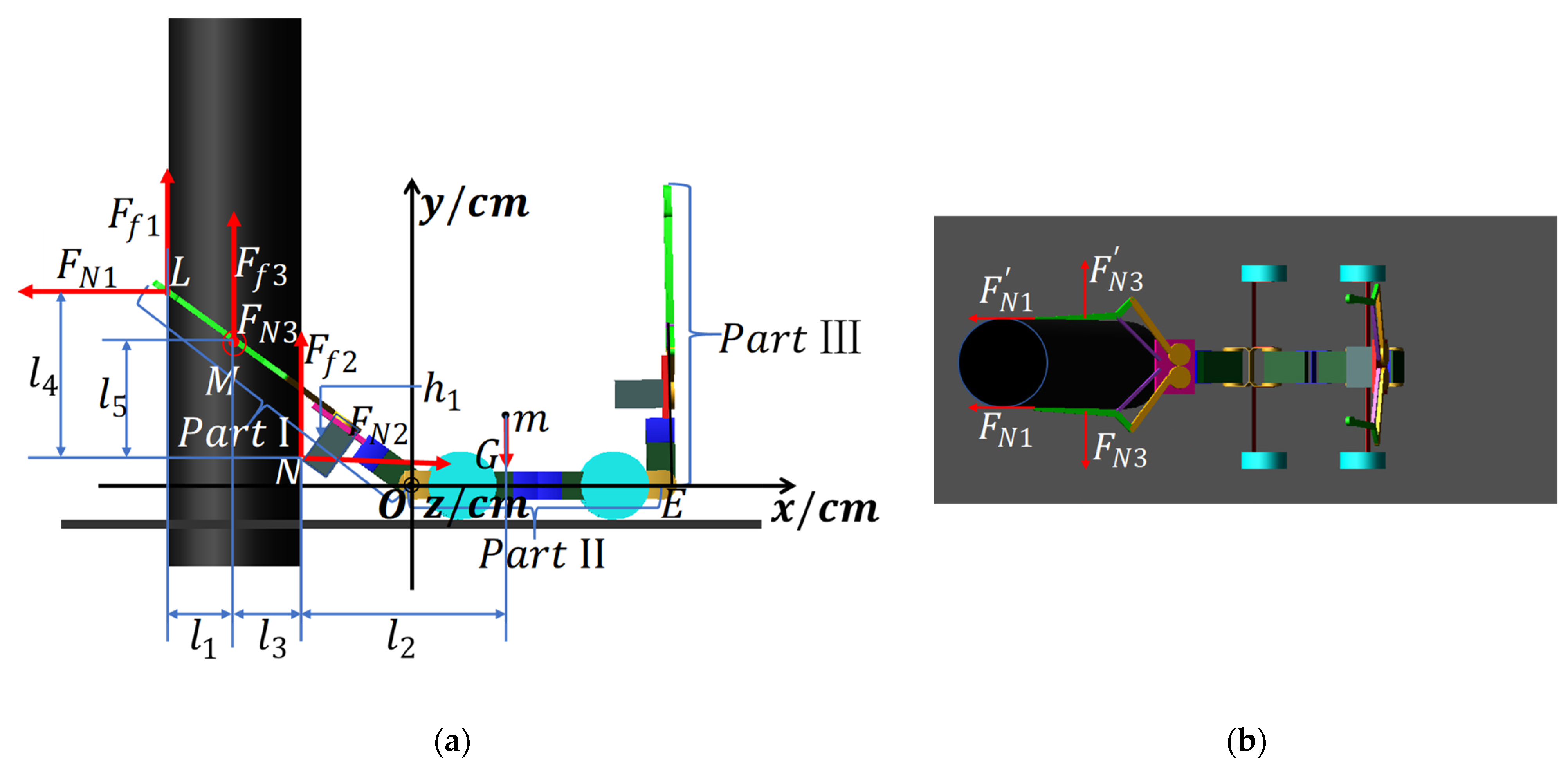
3.2. Force Analysis of Static State
3.3. Force Analysis of Dynamic Process
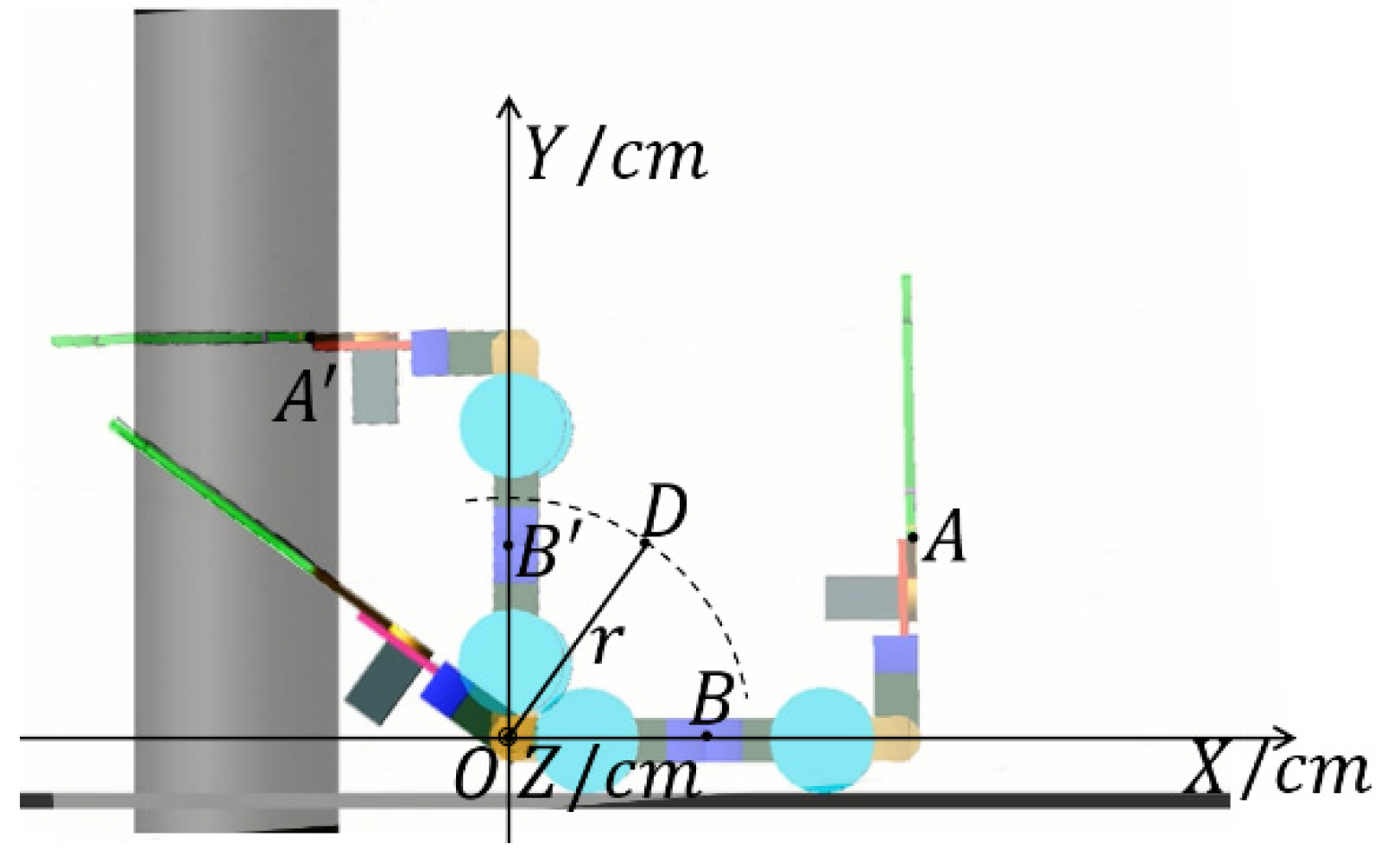
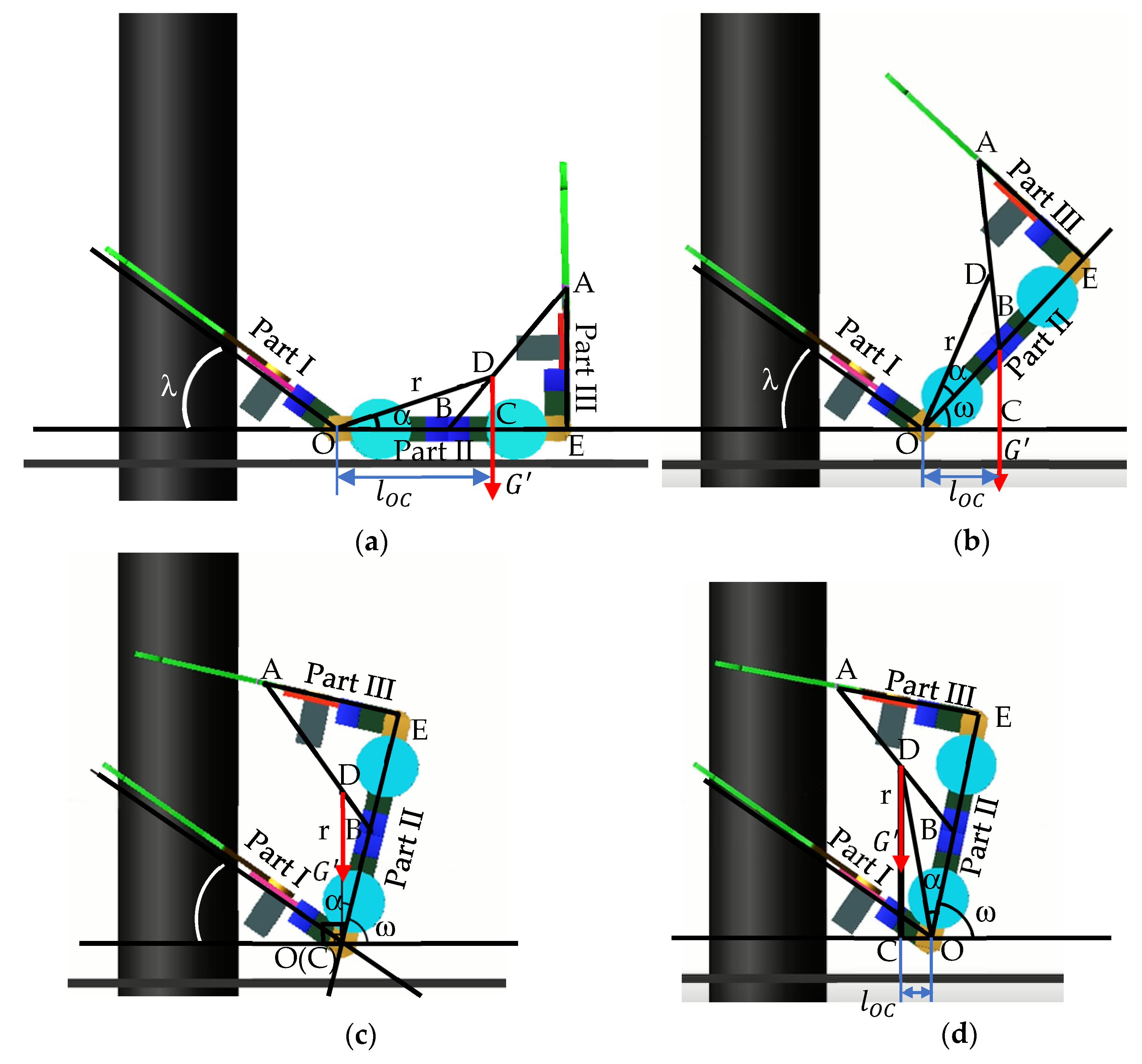
3.3.1. Analysis of the Trajectory of Mass Center
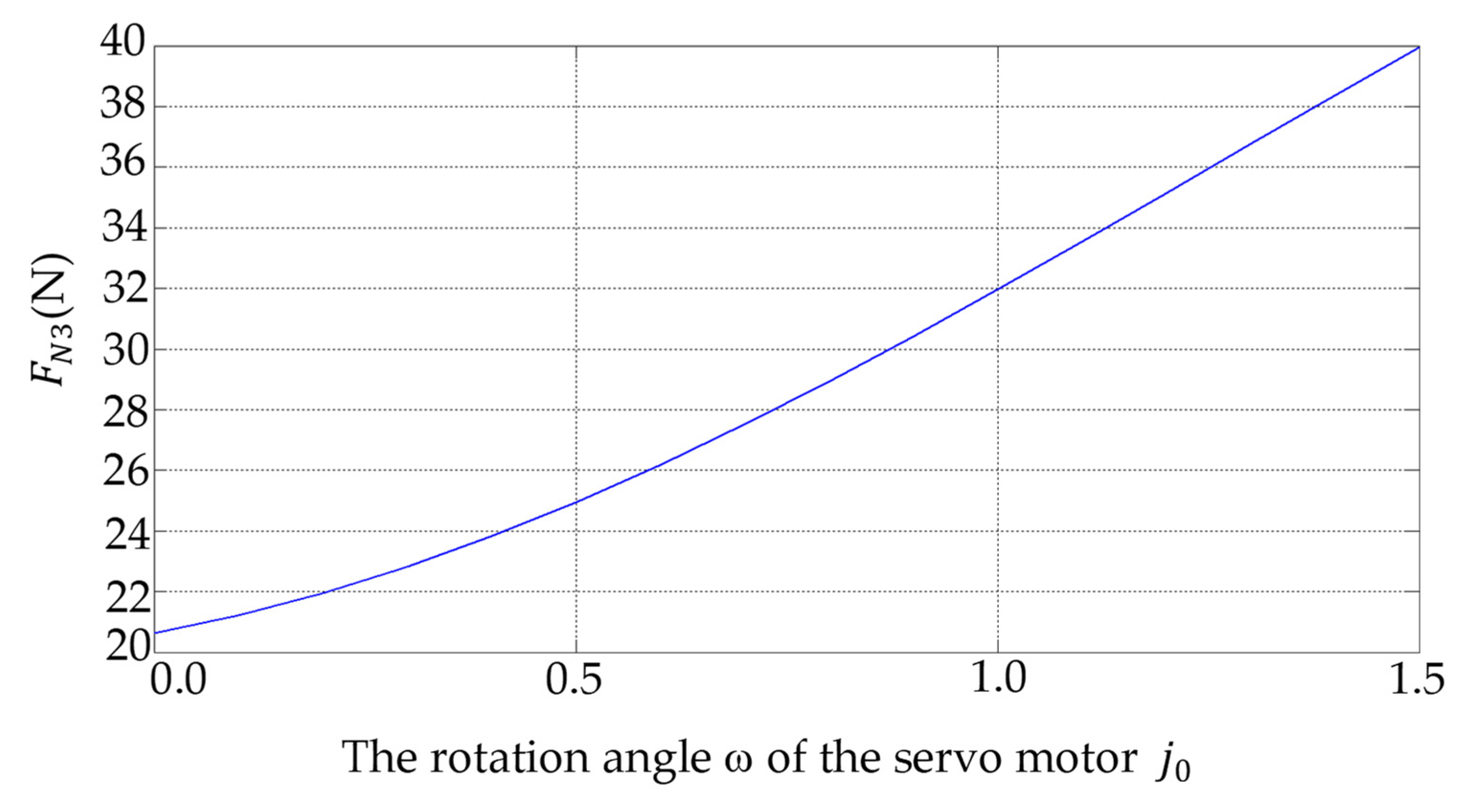
3.3.2. Torque Analysis of the WL_PCR
3.4. Load Analysis of the WL_PCR
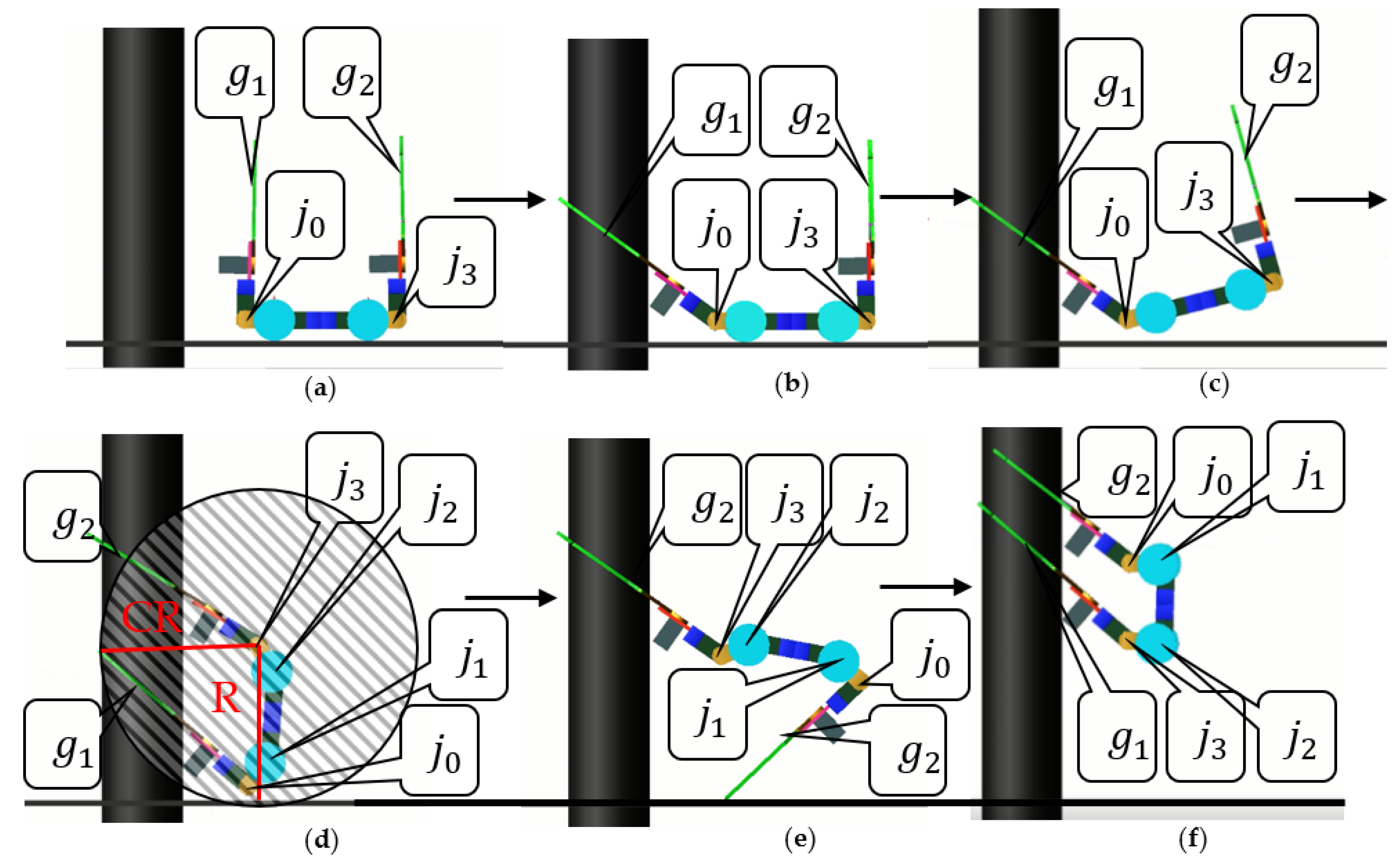
3.5. Flip Locomotion
3.5.1. Flip Condition
3.5.2. Control Scheme
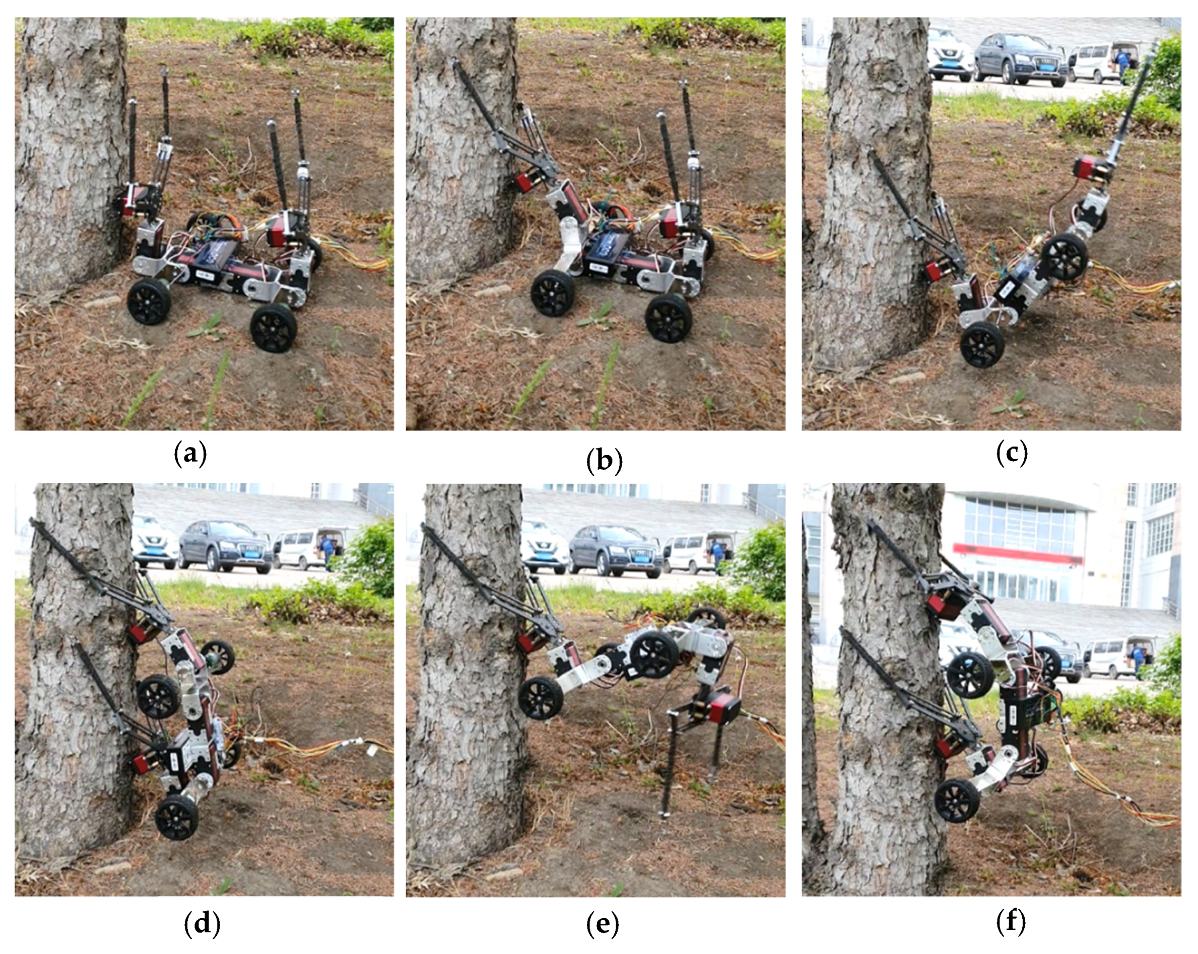
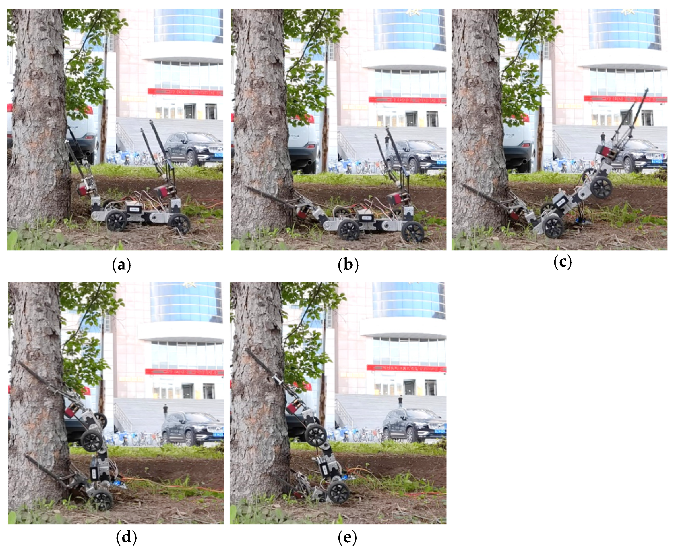
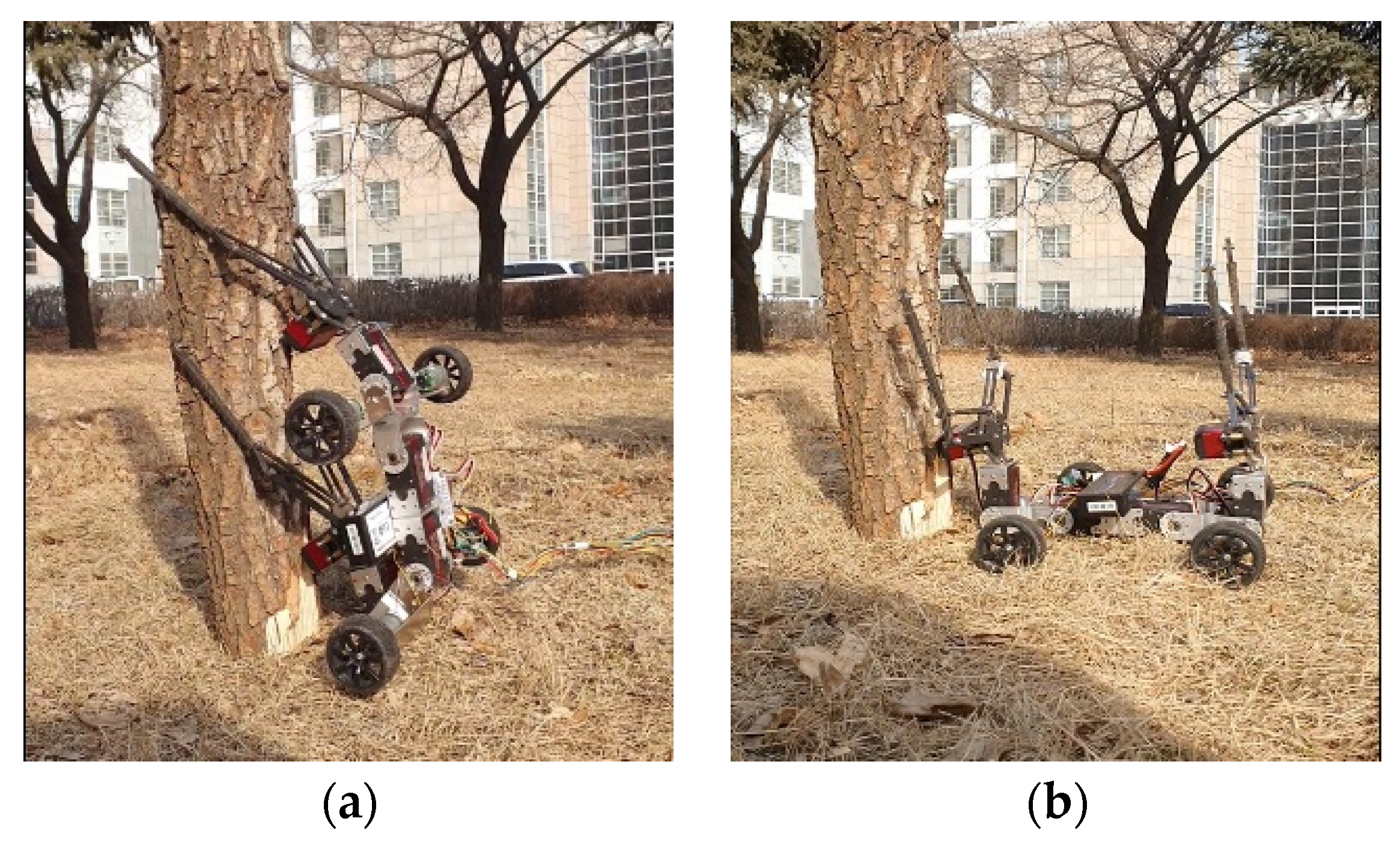
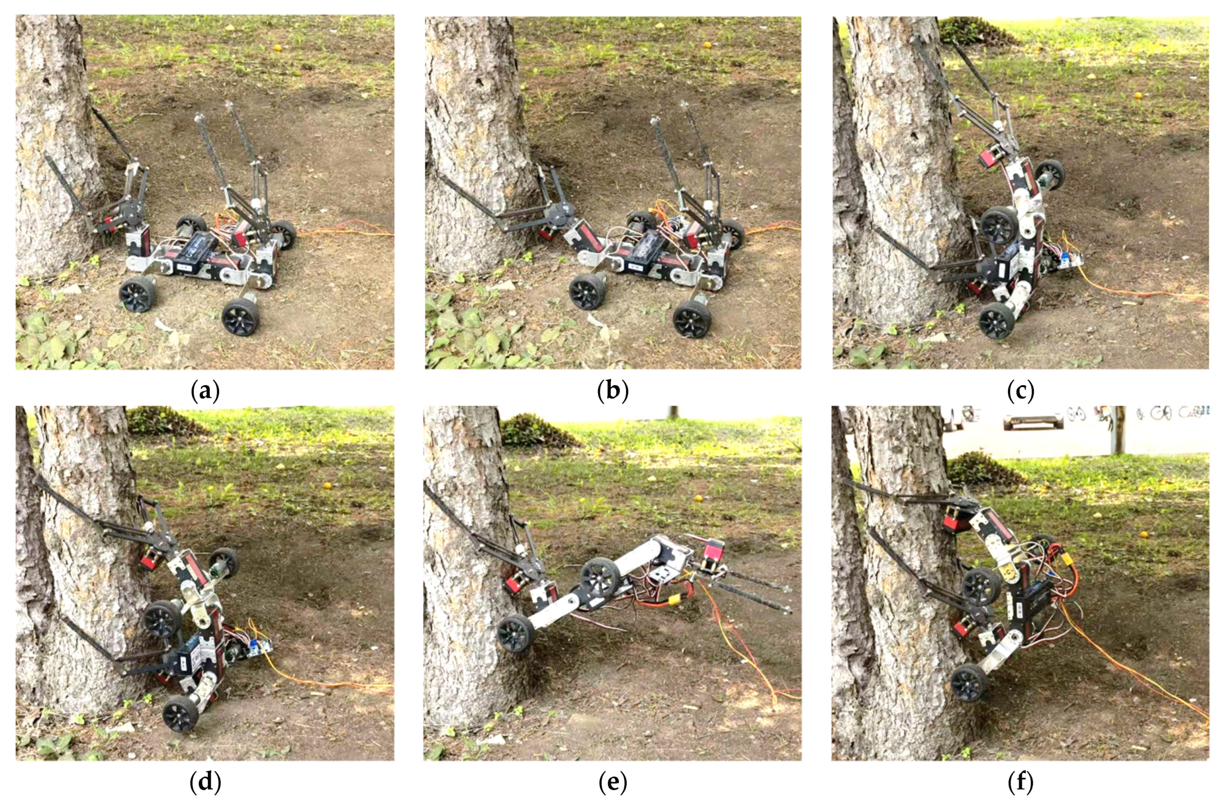
4. Experiments
5. Conclusions
Author Contributions
Funding
Institutional Review Board Statement
Informed Consent Statement
Data Availability Statement
Acknowledgments
Conflicts of Interest
Appendix A

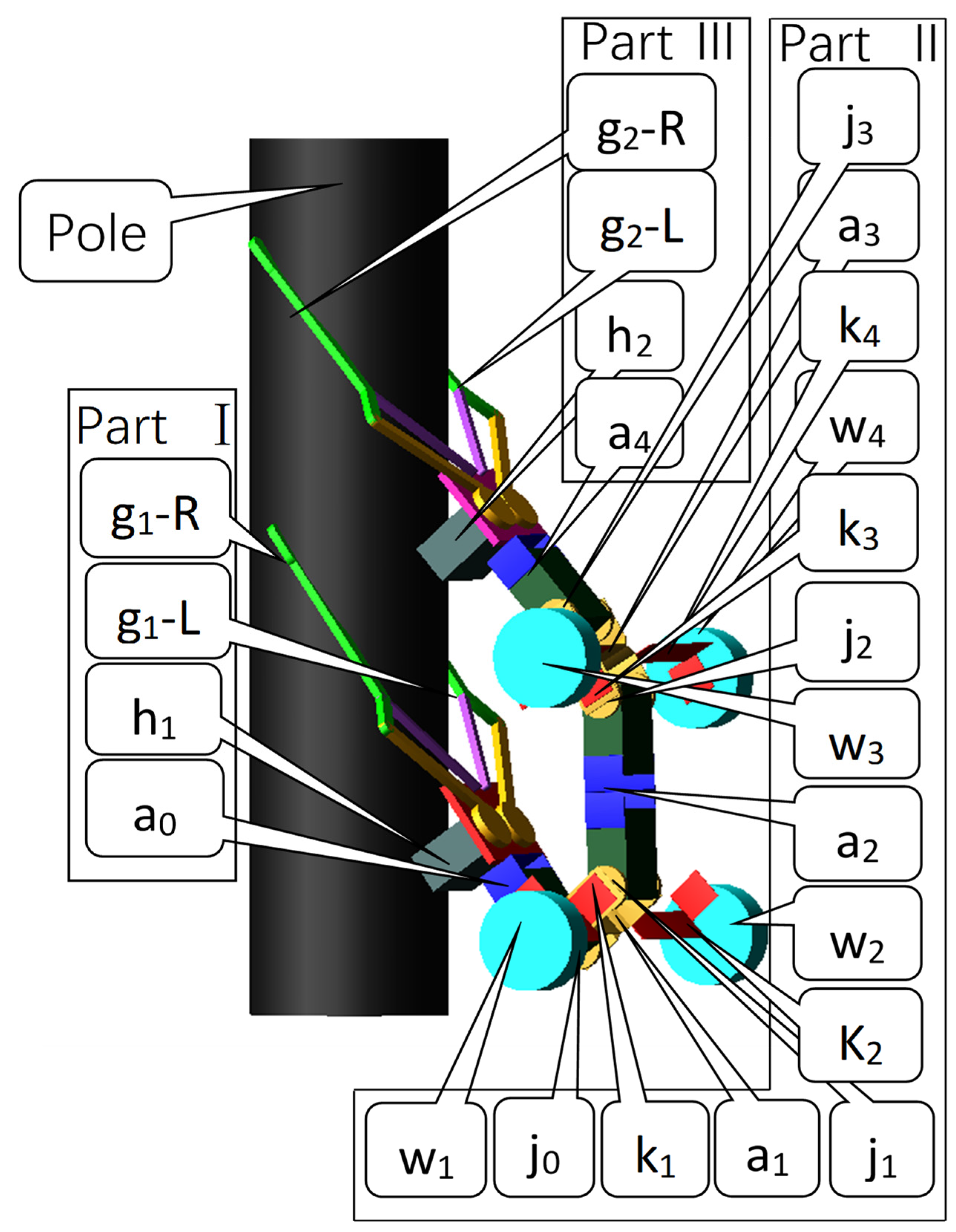
| Variable | Variable Name |
|---|---|
| bar linkages | , , , , |
| joints | , , , |
| supports | , |
| grippers | , |
| wheels | , , , |
| fixed poles | , , , |
| Contact point between robot’s Part I front end with pole | L |
| Contact point between robot’s Part I middle end with pole | M |
| Contact point between support with pole | N |
| Static friction coefficient at point L | |
| Static friction coefficient at point N | |
| Static friction coefficient at point M | |
| Acceleration of gravity | g |
| The supporting force of pole on the gripper at L point | , |
| The supporting force of pole on the gripper at M point | , |
| The supporting force of pole on the support at N point | |
| The frictional force between gripper with pole at L point | , |
| The frictional force between gripper with pole at M point | , |
| The frictional force between support with pole at N point | |
| Center of mass of robot | m |
| Gravity of robot | G |
| Arm of force , to point M | |
| Arm of force G to point N | |
| Arm of force to point M | |
| Arm of force , to point N | |
| Arm of force to point M | |
| Quality of Part I | |
| Quality of Part II | |
| Quality of Part III | |
| Quality of load | |
| The pressure exerted by the gripper on the pole | |
| Maximum force provided by gripper | |
| Center of mass of Part II | B |
| Center of mass of Part III | A |
| Center of mass of Part II and Part III | D |
| Center of mass of Part II, Part III and load | |
| The position of | O |
| The position of | E |
| Gravity of Part II and Part III | |
| Arm of force to point O | |
| Distance between point O and D | r |
| Distance between point O and | |
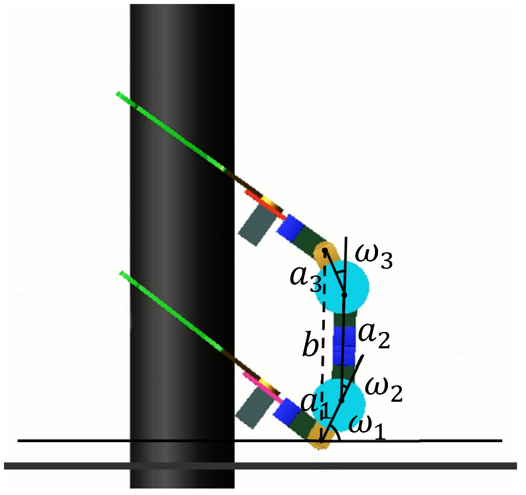
| The angle between and OE | α |
| The angle between O and OE | |
| Angle between OE and horizontal line | ω |
| Angle between Part I and horizontal line | λ |
| Torque of servomotor at when there is no load | |
| Torque of servomotor at when there is a load | |
| Gravity of robot and load | |
| Gravity of Part II, Part III and load | |
| Arm of force to point O | |
| The supporting force of pole on the gripper at M point when there is a load | |
| Distance from the top of the gripper to the support | a |
| Distance from to | b |
| Distance from the top of the gripper to . | CR |
| Diameter of pole | d |
| Distance from to the ground | e |
| Length of support | h |
| Distance from to the ground | R |
| Rotation angle of servomotor at | |
| Rotation angle of servomotor at | |
| Rotation angle of servomotor at | |
| Length of bar linkage | |
| Length of bar linkage | |
| Length of bar linkage |
References
- Yao, M.; Zhou, Y.; Zhang, Z.; He, B.; Sun, R.; Zhang, X. The Measuring Method of the Inner Deformation for High Concrete Faced Rockfill Dam with Pipe-robot Monitoring System. In Proceedings of the 2016 10th International Conference on Sensing Technology, Nanjing, China, 11–13 November 2016. [Google Scholar]
- Hung Manh, L.; Tran Hiep, D.; Nhan Huu, P.; Quang Phuc, H.; Anh Quyen, P. Automated robotic monitoring and inspection of steel structures and bridges. Robotica 2019, 37, 947–967. [Google Scholar]
- Enjikalayil Abdulkader, R.; Veerajagadheswar, P.; Htet Lin, N.; Kumaran, S.; Vishaal, S.R.; Elara, M.R. Sparrow: A Magnetic Climbing Robot for Autonomous Thickness Measurement in Ship Hull Maintenance. J. Mar. Sci. Eng. 2020, 8, 469. [Google Scholar] [CrossRef]
- Lu, X.; Qiu, R.; Liu, G.; Huang, F. The Design of an Inspection Robot for Boiler Tubes Inspection. In Proceedings of the 2009 International Conference on Artificial Intelligence and Computational Intelligence, Shanghai, China, 7–8 November 2009; pp. 313–317. [Google Scholar] [CrossRef]
- Guan, Y.; Jiang, L.; Zhu, H.; Wu, W.; Zhou, X.; Zhang, H.; Zhang, X. Climbot: A Bio-Inspired Modular Biped Climbing Robot-System Development, Climbing Gaits, and Experiments. J. Mech. Robot.-Trans. ASME 2016, 8, 021026. [Google Scholar] [CrossRef]
- Chen, W.; Gu, S.; Zhu, L.; Zhang, H.; Zhu, H.; Guan, Y. Representation of truss-style structures for autonomous climbing of biped pole-climbing robots. Robot. Auton. Syst. 2018, 101, 126–137. [Google Scholar] [CrossRef]
- Kamedula, M.; Tsagarakis, N.G. Reactive Support Polygon Adaptation for the Hybrid Legged-Wheeled CENTAURO Robot. IEEE Robot. Autom. Lett. 2020, 5, 1734–1741. [Google Scholar] [CrossRef]
- Ceilinger, M.; Poranne, R.; Desai, R.; Thomaszewski, B.; Coros, S. Skaterbots: Optimization-based design and motion synthesis for robotic creatures with legs and wheels. ACM Trans. Graph. 2018, 37, 1–12. [Google Scholar] [CrossRef] [Green Version]
- Wei, Z.; Song, G.; Qiao, G.; Zhang, Y.; Sun, H. Design and Implementation of a Leg-Wheel Robot: Transleg. J. Mech. Robot.-Trans. ASME 2017, 9, 051001. [Google Scholar] [CrossRef]
- Du, Q.; Lu, X.; Wang, Y.; Liu, S. The obstacle-surmounting analysis of a pole-climbing robot. Int. J. Adv. Robot. Syst. 2020, 17, 17. [Google Scholar]
- Guo, Y.; Zhang, J.; Ju, Y.; Guo, X. Climbing Reconnaissance Drone Design. In Proceedings of the 2018 3rd International Conference on Insulating Materials, Material Application and Electrical Engineering, IMMAEE 2018, Melbourne, VIC, Australia, 15–16 September 2018. [Google Scholar]
- Xi, F.; Jiang, Q. Dynamic obstacle-surmounting analysis of a bilateral-wheeled cable-climbing robot for cable-stayed bridges. Ind. Robot-Int. J. Robot. Res. Appl. 2019, 46, 431–443. [Google Scholar]
- Asgari, M.; Nikoobin, A. Analysis of Optimal Dynamic Manipulation for Robotic Manipulator Based on Pontryagin’s Minimum Principle. Arab. J. Sci. Eng. 2020, 45, 9159–9169. [Google Scholar] [CrossRef]
- Arutyunov, A.; Karamzin, D. A Survey on Regularity Conditions for State-Constrained Optimal Control Problems and the Non-degenerate Maximum Principle. J. Optim. Theory Appl. 2020, 184, 697–723. [Google Scholar] [CrossRef]
- Sands, T. Optimization Provenance of Whiplash Compensation for Flexible Space Robotics. Aerospace 2019, 6, 93. [Google Scholar] [CrossRef] [Green Version]
- Mohamed, A.; Ren, J.; Huang, X.S.; Ouda, A.N.; Abdo, G.M. Comparative study of dynamic programming and Pontryagin’s minimum principle for autonomous multi-wheeled combat vehicle path planning. Int. J. Heavy Veh. Syst. 2019, 26, 565–577. [Google Scholar] [CrossRef]
- Rathinam, S.; Manyam, S.G.; Zhang, Y.T. Near-Optimal Path Planning for a Car-Like Robot Visiting a Set of Waypoints With Field of View Constraints. IEEE Robot. Autom. Lett. 2019, 4, 391–398. [Google Scholar] [CrossRef]
- Nikoobin, A.; Moradi, M. Analysis of Optimal Balancing for Robotic Manipulators in Repetitive Motions. J. Dyn. Syst. Meas. Control-Trans. ASME 2018, 140, 8. [Google Scholar] [CrossRef]
- Diveev, A.; Shmalko, E.; Serebrenny, V.; Zentay, P. Fundamentals of Synthesized Optimal Control. Mathematics 2020, 9, 21. [Google Scholar] [CrossRef]
- Shah, R.; Sands, T. Comparing Methods of DC Motor Control for UUVs. Appl. Sci. 2021, 11, 4972. [Google Scholar] [CrossRef]
- Hu, H.J.; Zhu, S.Y.; Cui, P.Y. Desensitized optimal trajectory for landing on small bodies with reduced landing error. Aerosp. Sci. Technol. 2016, 48, 178–185. [Google Scholar] [CrossRef]
- Makkapati, V.R.; Dor, M.; Tsiotras, P. Trajectory Desensitization in Optimal Control Problems. In Proceedings of the 2018 IEEE Conference on Decision and Control, Miami Beach, FL, USA, 17–19 December 2018; pp. 2478–2483. [Google Scholar]
- Papadimitriou, A.; Andrikopoulos, G.; Nikolakopoulos, G. On the Optimal Adhesion Control of a Vortex Climbing Robot. J. Intell. Robot. Syst. 2021, 102, 1–15. [Google Scholar] [CrossRef]
- Boggs, P.T.; Tolle, J.W. Sequential quadratic programming for large-scale nonlinear optimization. J. Comput. Appl. Math. 2000, 124, 123–137. [Google Scholar] [CrossRef]
- Xu, J.X.; Wang, W. Two optimization algorithm for solving robotics inverse kinematics with redundancy. In Proceedings of the 2007 IEEE International Conference on Control and Automation, Guangzhou, China, 30 May–1 June 2007; IEEE: New York, NY, USA, 2007; pp. 1142–1149. [Google Scholar]
- Du, Q.; Li, Y.; Liu, S. Design of a micro pole-climbing robot. Int. J. Adv. Robot. Syst. 2019, 16, 1729881419852813. [Google Scholar]
- Xie, D.; Liu, J.; Kang, R.; Zuo, S. Fully 3D-Printed Modular Pipe-Climbing Robot. IEEE Robot. Autom. Lett. 2021, 6, 462–469. [Google Scholar] [CrossRef]
- Grigore, L.S.; Gorgoteanu, D.; Molder, C.; Alexa, O.; Oncioiu, I.; Stefan, A.; Constantin, D.; Lupoae, M.; Balasa, R.-I. A Dynamic Motion Analysis of a Six-Wheel Ground Vehicle for Emergency Intervention Actions. Sensors 2021, 21, 1618. [Google Scholar] [CrossRef] [PubMed]
- Qi, L.; Zhang, T.; Xu, K.; Pan, H.; Zhang, Z.; Yuan, Y. A novel terrain adaptive omni-directional unmanned ground vehicle for underground space emergency: Design, modeling and tests. Sustain. Cities Soc. 2021, 65, 102621. [Google Scholar] [CrossRef]


| Motor Brand | Bi Hui |
|---|---|
| Rated voltage | 6 V |
| Rated current | 0.42 A |
| Rated power | 2 W |
| Speed | 4900 m/min |
| Torque | 40 g∙cm |
| Motor weight | 68 g |
| Motor Brand | Dsservo |
|---|---|
| Rated voltage | 7.4 V |
| Maximum current | 5 A |
| Controllable angle | 270° |
| Torque | 60 kg∙cm |
| Motor weight | 158 g |
| Components | Dimensions (cm) |
|---|---|
| 6.3 | |
| 6.8 | |
| 12.4 | |
| 6.8 | |
| 6.3 | |
| 4.8 | |
| 4.8 | |
| 25.7 | |
| 25.7 | |
| 10.0 | |
| 10.0 | |
| 10.0 | |
| 10.0 |
| Part | Weight (kg) |
|---|---|
| Part I | 0.737 |
| Part II | 1.206 |
| Part III | 0.737 |
| Parameters | λ | b (cm) | |||
|---|---|---|---|---|---|
| 1 | 48° | 90° | 0° | 0° | 26.0 |
| 2 | 48° | 0° | 90° | 90° | 12.4 |
| 3 | 48° | 63° | 26° | 28° | 24.5 |
Publisher’s Note: MDPI stays neutral with regard to jurisdictional claims in published maps and institutional affiliations. |
© 2021 by the authors. Licensee MDPI, Basel, Switzerland. This article is an open access article distributed under the terms and conditions of the Creative Commons Attribution (CC BY) license (https://creativecommons.org/licenses/by/4.0/).
Share and Cite
Wang, Y.; Du, Q.; Zhang, T.; Xue, C. The WL_PCR: A Planning for Ground-to-Pole Transition of Wheeled-Legged Pole-Climbing Robots. Robotics 2021, 10, 96. https://doi.org/10.3390/robotics10030096
Wang Y, Du Q, Zhang T, Xue C. The WL_PCR: A Planning for Ground-to-Pole Transition of Wheeled-Legged Pole-Climbing Robots. Robotics. 2021; 10(3):96. https://doi.org/10.3390/robotics10030096
Chicago/Turabian StyleWang, Yankai, Qiaoling Du, Tianhe Zhang, and Chengze Xue. 2021. "The WL_PCR: A Planning for Ground-to-Pole Transition of Wheeled-Legged Pole-Climbing Robots" Robotics 10, no. 3: 96. https://doi.org/10.3390/robotics10030096
APA StyleWang, Y., Du, Q., Zhang, T., & Xue, C. (2021). The WL_PCR: A Planning for Ground-to-Pole Transition of Wheeled-Legged Pole-Climbing Robots. Robotics, 10(3), 96. https://doi.org/10.3390/robotics10030096