
Multi AGV Coordination Tolerant to Communication Failures


Abstract
1. Introduction
2. State of the Art
3. Overall System Architecture and Lower Level Control
4. Modified TEA* Algorithm
- Implementation of a Task Scheduling function;
- Modification of the method that associates the current robot position with a node from the graph;
- Implementation of an algorithm that creates a binary semaphore when a communication fault is detected.
4.1. Task Scheduling
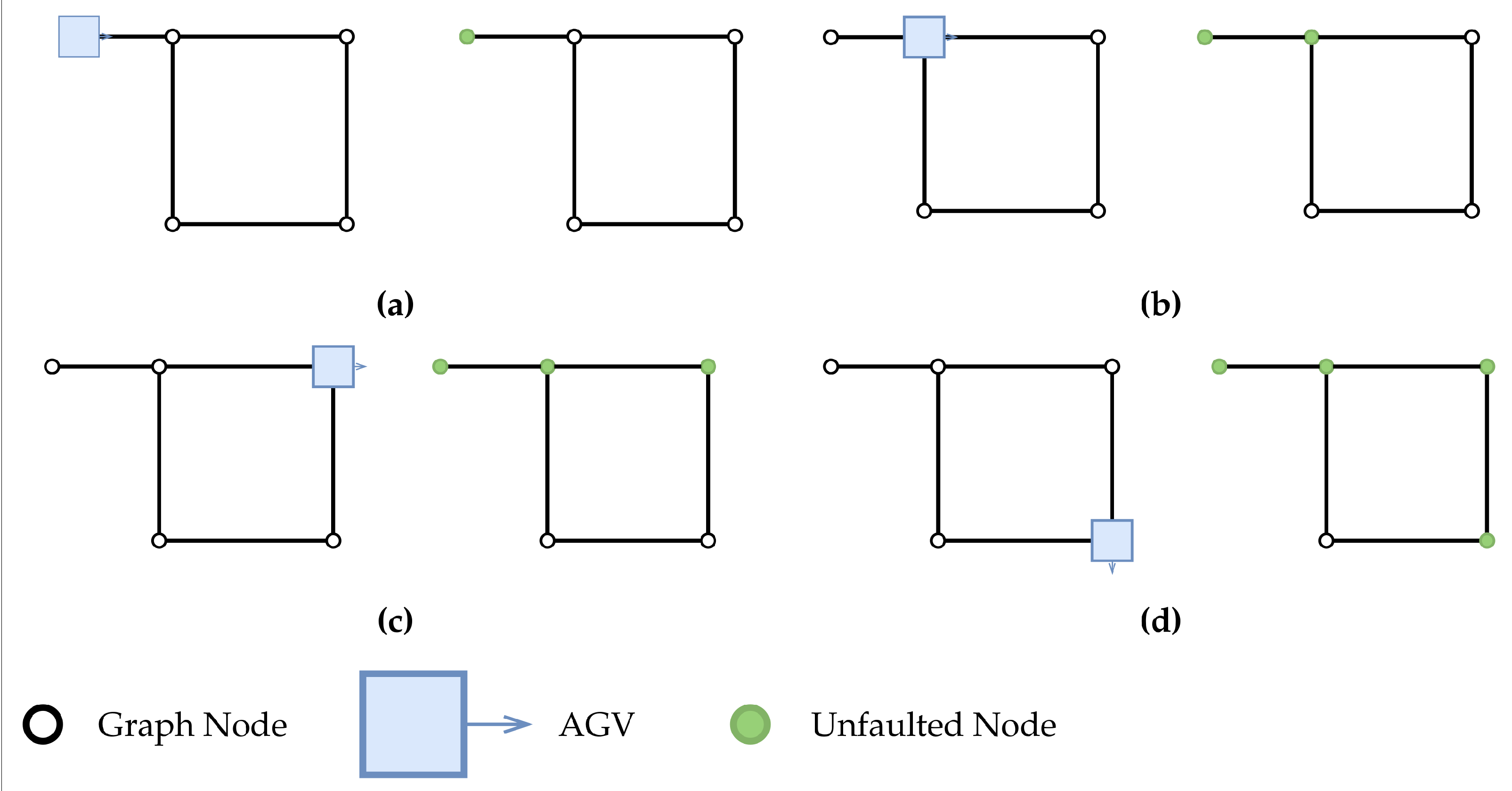
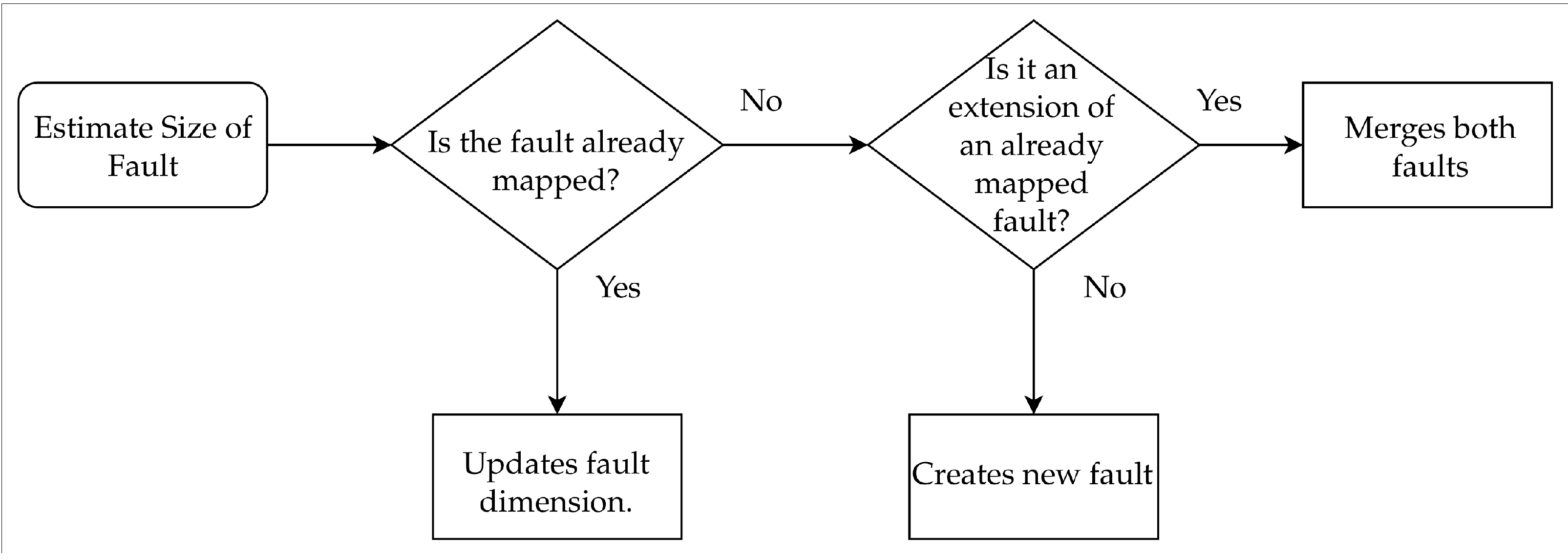
4.2. Planning during Communication Faults
5. Supervision Module
5.1. Planning Supervision Sub-Module (PSSM)
- Check whether any robots are too distant from their supposed position;
- Check whether the maximum difference between steps is 1;
- Check whether any robot is moving to a position currently occupied by another robot.
- Robot is stopped;
- Robot is rotating;
- Robot is currently moving along a link.
5.2. Communication Supervision Sub-Module (CSSM)
- Situations where one area in the factory floor map consistently has no communication with the central control unit;
- Situations where temporary loss of connection happens with the central control unit.
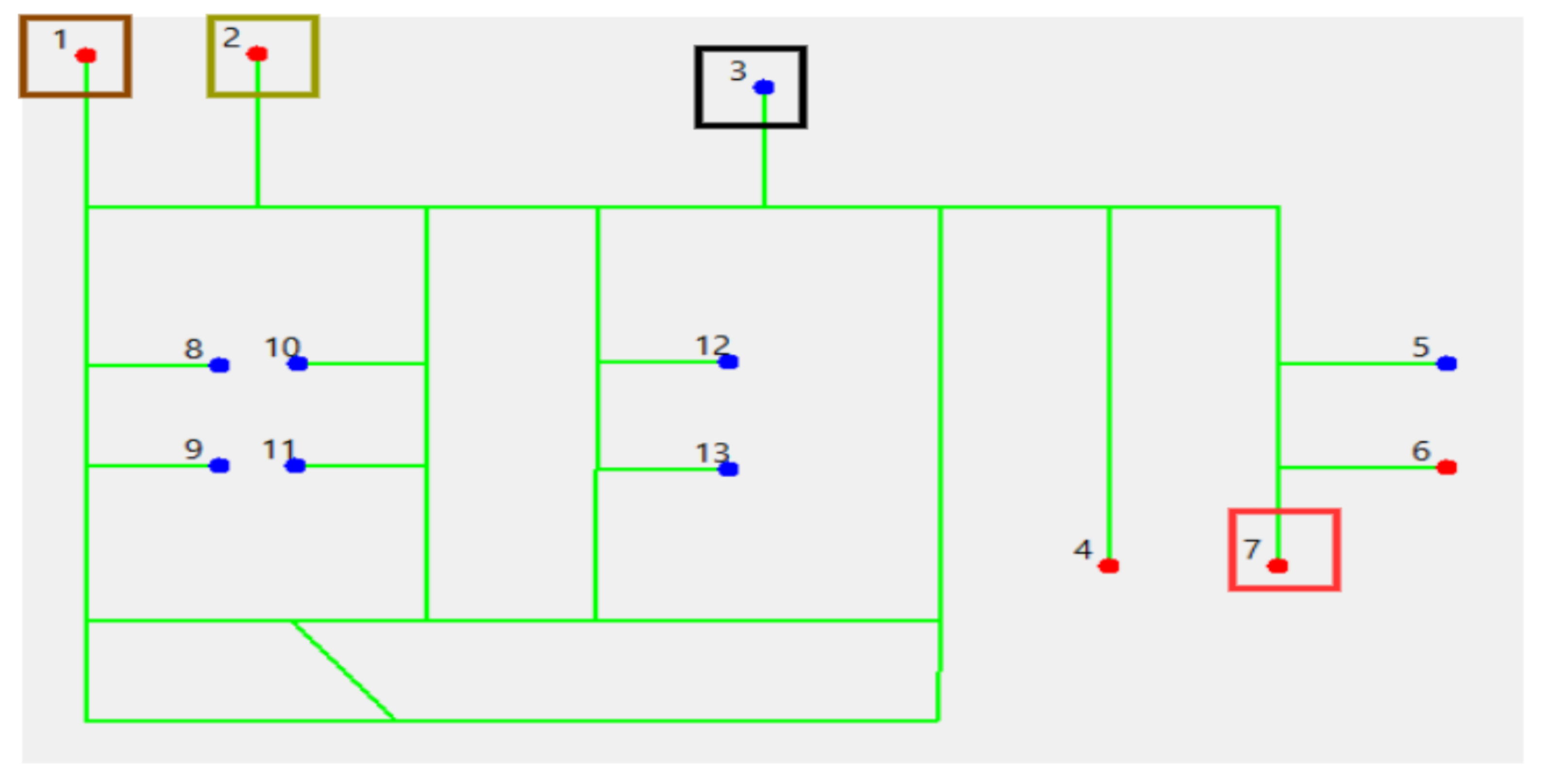
6. Tests and Validation
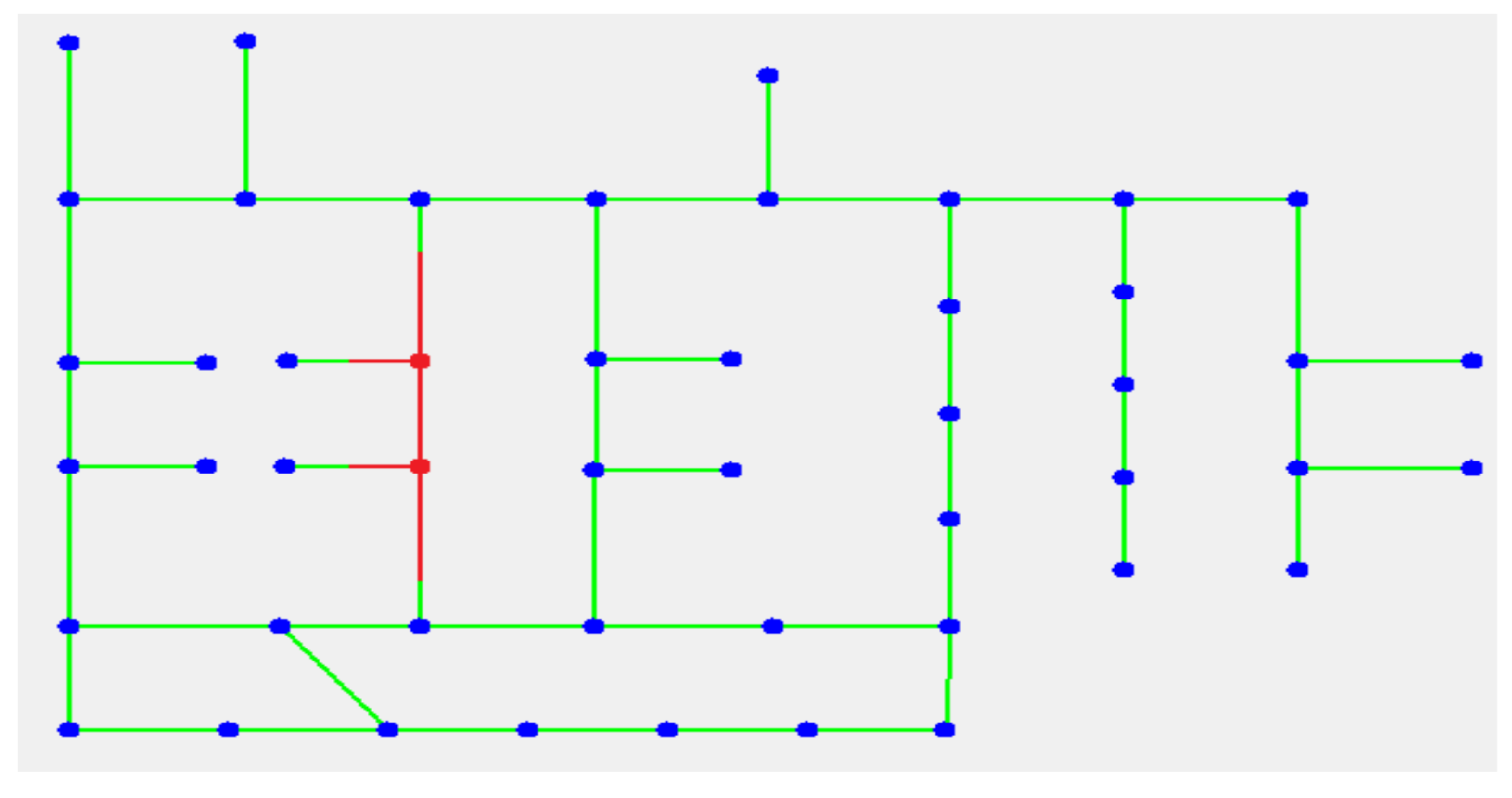
6.1. Planning Supervision and Overall System Performance when Subjected to Static Communication Faults
6.2. Planning Supervision and Overall System Performance when Subjected to Static and Sporadic Communication Faults
6.3. Cases Where the Implemented System Can’t Guarantee a Safe Execution of the Mission
- Two or more robots entering the same fault at the same time;
- Impossibility of a robot to move away from the exit node of a fault.
7. Conclusions
Author Contributions
Funding
Institutional Review Board Statement
Informed Consent Statement
Data Availability Statement
Acknowledgments
Conflicts of Interest
Abbreviations
| TEA* | Time Enhanced A* |
| AGV | Autonomous ground vehicle |
| MAPF | Multi-Agent Pathfinding |
| LPA* | Lifelong Planning A* |
| Mutex | Multiple exclusion object |
| NP | Non-deterministic Polynomial-Time |
| PSSM | Planning Supervision Sub-Module |
| CSSM | Communication Supervision Sub-Module |
Appendix A. Execution of the First Mission with no Communication Faults


Appendix B. Execution of the Second Mission with no Communication Faults


Appendix C. Execution of a Mission with Static Communication Faults


Appendix D. Execution of a Mission with Static and Sporadic Communication Faults


Appendix E. Video Links
References
- Ullrich, G. The History of Automated Guided Vehicle Systems. Autom. Guid. Veh. Syst. Prim. Pract. Appl. 2015. [Google Scholar] [CrossRef]
- Siefke, L.; Sommer, V.; Wudka, B.; Thomas, C. Robotic systems of systems based on a decentralized service-oriented architecture. Robotics 2020, 9, 78. [Google Scholar] [CrossRef]
- Santos, J.; Costa, P.; Rocha, L.F.; Moreira, A.P.; Veiga, G. Time enhanced A*: Towards the development of a new approach for Multi-Robot Coordination. In Proceedings of the IEEE International Conference on Industrial Technology (ICIT), Seville, Spain, 17–19 March 2015; pp. 3314–3319. [Google Scholar] [CrossRef]
- Moura, P.; Costa, P.; Lima, J.; Costa, P. A temporal optimization applied to time enhanced A*. AIP Conf. Proc. 2019, 2116, 1–4. [Google Scholar] [CrossRef]
- Downey, A.B. The Little Book of Semaphores, 2nd ed.; v2.2.1; ; Green Tea Press: Needham, MA, USA, 2016. [Google Scholar]
- Atzmon, D.; Stern, R.; Felner, A.; Wagner, G.; Barták, R.; Zhou, N.F. Robust multi-agent path finding and executing. J. Artif. Intell. Res. 2020, 67, 549–579. [Google Scholar] [CrossRef]
- Felner, A.; Stern, R.; Shimony, S.E.; Boyarski, E.; Goldenberg, M.; Sharon, G.; Sturtevant, N.; Wagner, G.; Surynek, P. Search-based optimal solvers for the multi-agent pathfinding problem: Summary and challenges. In Proceedings of the 10th Annual Symposium on Combinatorial Search, SoCS 2017, Pittsburgh, PA, USA, 16–17 June 2017; pp. 29–37. [Google Scholar]
- Surynek, P. An optimization variant of multi-robot path planning is intractable. In Proceedings of the National Conference on Artificial Intelligence, Atlanta, GA, USA, 11–15 July 2010; Volume 2, pp. 1261–1263. [Google Scholar]
- Yu, J. Intractability of optimal multirobot path planning on planar graphs. IEEE Robot. Automat. Lett. 2016, 1, 33–40. [Google Scholar] [CrossRef]
- Falcó, A.; Hilario, L.; Montés, N.; Mora, M.C.; Nadal, E. A Path Planning Algorithm for a Dynamic Environment Based on Proper Generalized Decomposition. Mathematics 2020, 8, 2245. [Google Scholar] [CrossRef]
- Bae, H.; Kim, G.; Kim, J.; Qian, D.; Lee, S. Multi-robot path planning method using reinforcement learning. Appl. Sci. 2019, 9, 3057. [Google Scholar] [CrossRef]
- Yu, J.; Su, Y.; Liao, Y. The Path Planning of Mobile Robot by Neural Networks and Hierarchical Reinforcement Learning. Front. Neurorobot. 2020, 14, 1–12. [Google Scholar] [CrossRef] [PubMed]
- Da Costa, P.L.C.G. Planeamento Cooperativo de Tarefas e Trajectórias em Múltiplos Robôs. Ph.D. Thesis, Faculdade de Engenharia da Universidade do Porto, Porto, Portugal, 2011; p. 231. [Google Scholar]
- Latombe, J.C. Introduction and Overview. Robot Motion Planning. In Robot Motion Plan; Springer: Boston, MA, USA, 1991; pp. 1–57. [Google Scholar] [CrossRef]
- Lozano-Pérez, T.; Wesley, M.A. An Algorithm for Planning Collision-Free Paths Among Polyhedral Obstacles. Commun. ACM 1979, 22, 560–570. [Google Scholar] [CrossRef]
- LaValle, S.M. Planning Algorithms; Cambridge University Press: Cambridge, UK, 2006; 826p. [Google Scholar] [CrossRef]
- Hart, P.E.; Nilsson, N.J.; Raphael, B. The Heuristic Determination. IEEE Trans. Syst. Sci. Cybern. 1968, 100–107. [Google Scholar] [CrossRef]
- Stentz, A. Optimal and Efficient Path Planning/or Partially Known Environments. In Intelligent Unmanned Ground Vehicles; Springer: Boston, MA, USA, 1997. [Google Scholar]
- Koenig, S.; Likhachev, M. Incremental A*. In Advances in Neural Information Processing Systems 14 (NIPS 2001); Dietterich, T., Becker, S., Ghahramani, Z., Eds.; MIT Press: Cambridge, MA, USA, 2002. [Google Scholar]
- Wang, W.; Goh, W.B. Multi-robot path planning with the spatio-temporal A* algorithm and its variants. In Advanced Agent Technology, Proceedings of the AAMAS 2011, Taipei, Taiwan, 2–6 May 2011; Dechesne, F., Hattori, H., Mors, A., Such, J.M., Weyns, D., Eds.; Springer Publishing: New York, NY, USA, 2011; pp. 313–329. [Google Scholar] [CrossRef]
- Wagner, G.; Choset, H. Subdimensional expansion for multirobot path planning. Artif. Intell. 2015, 219, 1–24. [Google Scholar] [CrossRef]
- Jansen, R.; Tg, C.; Sturtevant, N. A new approach to cooperative pathfinding. In Proceedings of the 7th International Joint Conference on Autonomous Agents and Multiagent Systems, Taipei, Taiwan, 2–6 May 2008; Volume 3, pp. 1401–1404. [Google Scholar]
- Cao, Y.U.; Fukunaga, A.S.; Kahng, A.B. Cooperative Mobile Robotics: Antecedents and Directions. Auton. Robot. 1997, 4, 7–27. [Google Scholar] [CrossRef]
- Raynal, M. Fault-tolerant Agreement in Synchronous Message-passing Systems. In Synthesis Lectures on Distributed Computing Theory; Morgan & Claypool Publishers: Williston, VT, USA, 2010; Volume 1, pp. 1–189. [Google Scholar] [CrossRef]
- Kandath, H.; Senthilnath, J.; Sundaram, S. Mutli-agent consensus under communication failure using Actor-Critic Reinforcement Learning. In Proceedings of the 2018 IEEE Symposium Series on Computational Intelligence, SSCI 2018, Bangalore, India, 18–21 November 2019; pp. 1461–1465. [Google Scholar] [CrossRef]
- Braun, J.; Fernandes, L.A.; Moya, T.; Oliveira, V.; Brito, T.; Lima, J.; Costa, P. Robot@Factory Lite: An Educational Approach for the Competition with Simulated and Real Environment. In Proceedings of the Robot 2019: Fourth Iberian Robotics Conference, Porto, Portugal, 20–22 November 2019; pp. 478–489. [Google Scholar] [CrossRef]
- Costa, P.; Gonçalves, J.; Lima, J.; Malheiros, P. Simtwo realistic simulator: A tool for the development and validation of robot software. Theory Appl. Math. Comput. Sci. 2011, 1, 17–33. [Google Scholar]
- Silver, D. Cooperative pathfinding. In Proceedings of the Artificial Intelligence and Interactive Digital Entertainment Conference (AIIDE) 2005, Marina del Rey, CA, USA, 1–3 June 2005; pp. 117–122. [Google Scholar]


| Id Robot | Colour | Initial Priority | Task |
|---|---|---|---|
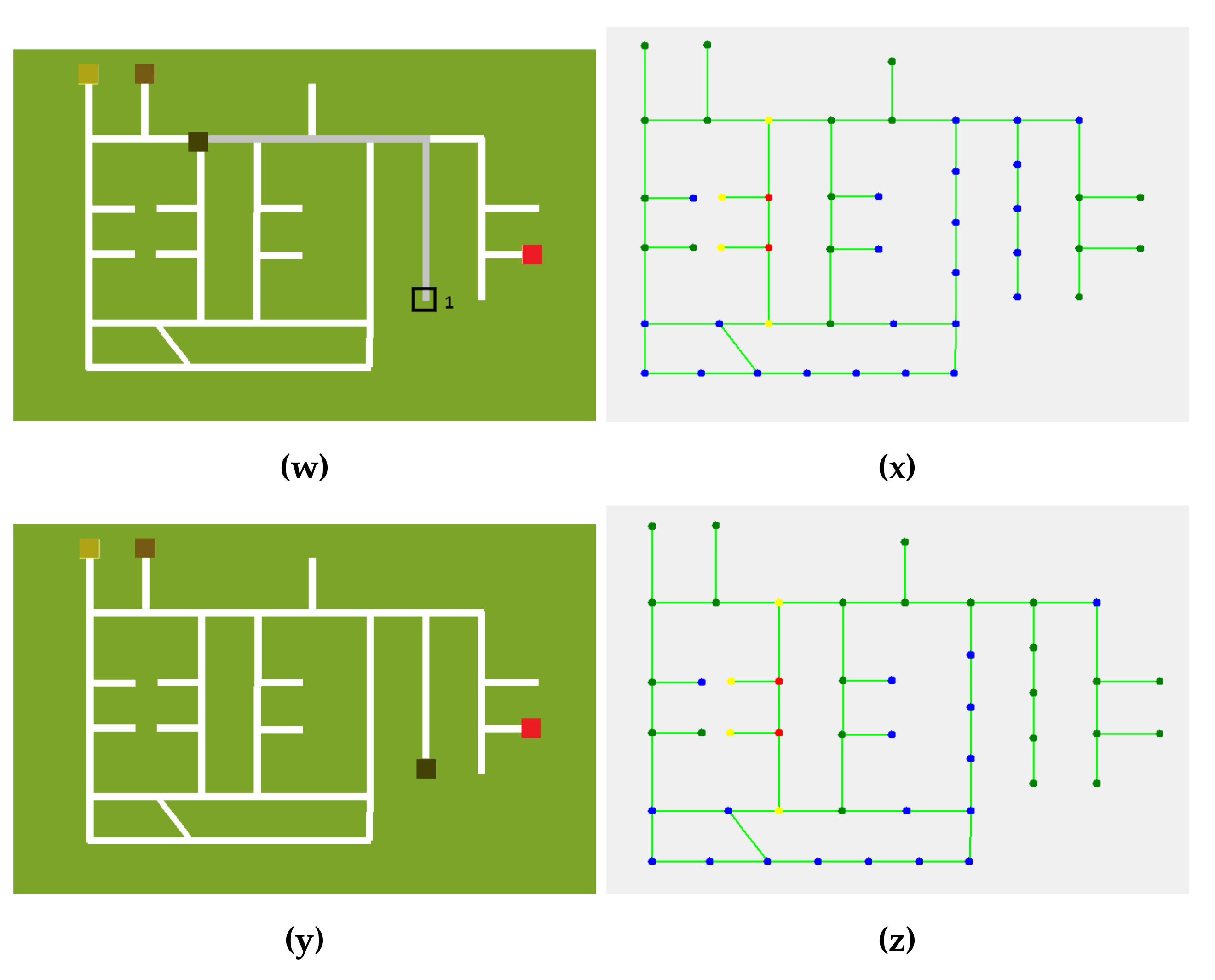
| 1 | Brown | 1 | 9 |
| 2 | Dark Green | 2 | 10 |
| 3 | Black | 3 | 11 |
| 4 | Red | 4 | 5 |
| Id Robot | Colour | Initial Priority | Task |
|---|---|---|---|
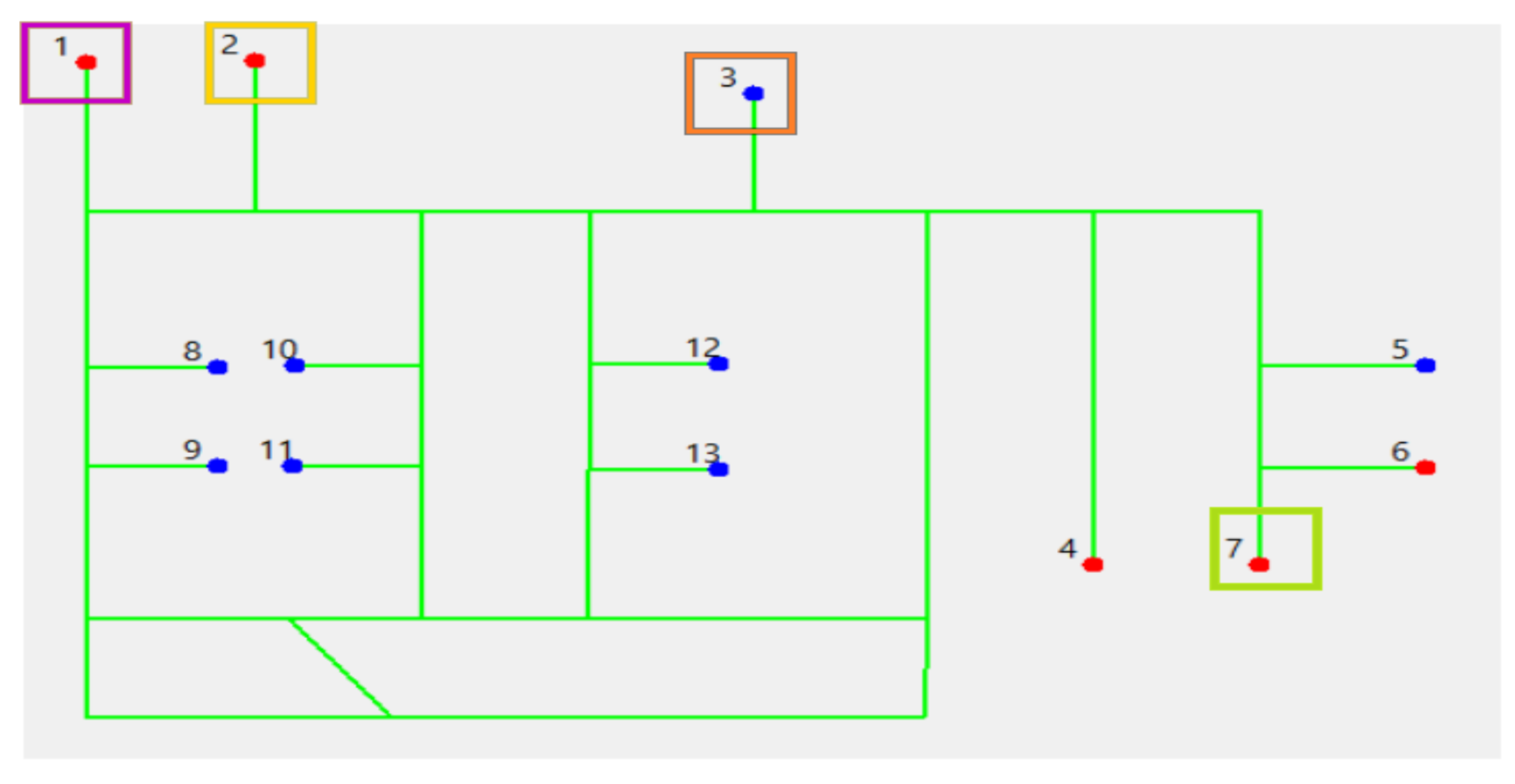
| 1 | Purple | 1 | 9 |
| 2 | Yellow | 2 | 10 |
| 3 | Orange | 3 | 11 |
| 4 | Green | 4 | 5 |
Publisher’s Note: MDPI stays neutral with regard to jurisdictional claims in published maps and institutional affiliations. |
© 2021 by the authors. Licensee MDPI, Basel, Switzerland. This article is an open access article distributed under the terms and conditions of the Creative Commons Attribution (CC BY) license (http://creativecommons.org/licenses/by/4.0/).
Share and Cite
Matos, D.; Costa, P.; Lima, J.; Costa, P. Multi AGV Coordination Tolerant to Communication Failures. Robotics 2021, 10, 55. https://doi.org/10.3390/robotics10020055
Matos D, Costa P, Lima J, Costa P. Multi AGV Coordination Tolerant to Communication Failures. Robotics. 2021; 10(2):55. https://doi.org/10.3390/robotics10020055
Chicago/Turabian StyleMatos, Diogo, Pedro Costa, José Lima, and Paulo Costa. 2021. "Multi AGV Coordination Tolerant to Communication Failures" Robotics 10, no. 2: 55. https://doi.org/10.3390/robotics10020055
APA StyleMatos, D., Costa, P., Lima, J., & Costa, P. (2021). Multi AGV Coordination Tolerant to Communication Failures. Robotics, 10(2), 55. https://doi.org/10.3390/robotics10020055