Abstract
Residue solvent accessibility is closely related to the spatial arrangement and packing of residues. Predicting the solvent accessibility of a protein is an important step to understand its structure and function. In this work, we present a deep learning method to predict residue solvent accessibility, which is based on a stacked deep bidirectional recurrent neural network applied to sequence profiles. To capture more long-range sequence information, a merging operator was proposed when bidirectional information from hidden nodes was merged for outputs. Three types of merging operators were used in our improved model, with a long short-term memory network performing as a hidden computing node. The trained database was constructed from 7361 proteins extracted from the PISCES server using a cut-off of 25% sequence identity. Sequence-derived features including position-specific scoring matrix, physical properties, physicochemical characteristics, conservation score and protein coding were used to represent a residue. Using this method, predictive values of continuous relative solvent-accessible area were obtained, and then, these values were transformed into binary states with predefined thresholds. Our experimental results showed that our deep learning method improved prediction quality relative to current methods, with mean absolute error and Pearson’s correlation coefficient values of 8.8% and 74.8%, respectively, on the CB502 dataset and 8.2% and 78%, respectively, on the Manesh215 dataset.
1. Introduction
Residue solvent accessibility (RSA) [1] in a protein is defined as the extent of accessible surface area of a given residue and is related to the residue spatial arrangement and packing. It reveals the folding state of proteins and has been considered as a significant quantitative measurement for three-dimensional structures of proteins [2]. Solvent accessibility is closely involved in structural domains’ identification [3], fold recognition [4], binding region identification [5], protein-protein interactions [6] and protein-ligand interactions [7]. Therefore, predicting the RSA of a protein represents an important step in determining its structure and function. Traditionally, RSA prediction is performed in two forms: (1) as a binary or multi-class classification problem with varying thresholds (two-state (exposed or buried) [8] or three-state (exposed, intermediate, or buried)) [9]; and (2) based on the relative accessible solvent area (rASA) prediction [10]. For example, if the surface area of a residue exceeds a threshold of 25%, the residue is classified as exposed; however, there is no standard definition of the thresholds for solvent-accessible area. Generally, the later approach is preferred over the former since rASA provides more information compared to binary or multi-class classification. For instance, it provides numerical values, which is required to apply this characteristic in protein structure and function prediction. In view of this, it is necessary to predict rASA. Recently, more and more studies have focused on rASA prediction.
Machine learning methods are extensively applied in RSA prediction and include those related to sequence alignment [11], neural networks [12,13,14,15], support vector machines [16,17], the use of multiple linear-regression models [18], Bayesian statistics [19], nearest-neighbor methods [20], energy optimization [21], gradient-boosted regression trees [22] and deep learning [23].
In 2003, Ahmad et al. [10] firstly detailed rASA prediction, and more attention has been paid to this research since that time. Ahmad et al. proposed a neural network method with only single sequence information as the input features, and the result of 18.8% mean absolute error (MAE) was achieved on the CB502 dataset. Wang et al. [18] applied the multiple linear regression method to predict rASA from the sequence information and position-specific scoring matrix (PSSM). This method achieved a result of 16.2% MAE on the CB502 dataset. Wang et al. [17] improved the result to 15.1% on the same dataset by accumulation cutoff set and support vector machine. Using a weighted sliding window scheme, Zhang et al. [24] obtained the result of 14% MAE on the CB502 dataset. Fan et al. [22] used gradient boosted regression trees to predict rASA and achieved a state-of-the-art performance, which is 9.4% MAE and 0.73 Pearson’s correlation coefficient (PCC) on the CB502 dataset. Another benchmark dataset Manesh215 [25] is also widely used by researchers [10,13,14,22,24,26] to validate prediction methods. Table 1 summarizes the recent developments in predicting the values of rASA.

Table 1.
The recent developments, in chronological order, for predicting the values of rASA.
Position-specific scoring matrix has been widely used in proteomics and bioinformatics, such as protein structure prediction [31,32], backbone angles [23],protein subcellular localization prediction [33,34,35], membrane protein type prediction [36,37,38], protein subchloroplast localization [39], etc. Protein-sequence coding and PSSM have also been used for RSA prediction [12,16,20]. Recently, other sequence-based features, such as physical properties [40], conservation score [41] and side-chain environment [42], have been used [20,21,22,23]. Additionally, properties predicted by computational methods have also been used, including those associated with evaluating secondary structure and protein disorder [21,22,43]. For most of these, standard labels for RSA areas are calculated by DSSP software [44]. The rASA is obtained by normalizing the ASA value over the maximum value of exposed surface area obtained for either (1) each amino acid or for (2) an extended tripeptide conformation of Ala-X-Ala or Gly-X-Gly [10].
Although these methods for RSA prediction have progressed, RSA prediction remains challenging. Improved performance in these areas will enable more precision in related protein studies.
Recently, deep learning methods have dramatically improved the state-of-the-art in speech recognition, visual object recognition, object detection and many other domains [45]. The Recurrent Neural Network (RNN), a type of deep neural network, processes an input sequence one element at a time, maintaining a hidden vector that implicitly contains the history information about the past elements of the sequence. RNN is an extremely powerful sequence model for sequence modeling tasks [46], and many RNN methods have been applied to protein structure and function prediction [47,48,49]. We focused on a RNN model specific to protein sequences and applied a bidirectional recurrent neural network (BRNN) to predict RSA. To capture more local and long-range information, a merging operator was used to merge bidirectional information, given that this has rarely been addressed previously. Our deep learning method, a stacked deep bidirectional recurrent neural network (SDBRNN), is proposed, with three-layer bidirectional long-short memory (BLSTM) network with different merging operators used in each hidden layer. The public benchmark datasets CB502, Manesh215 and CASP10 were used for testing, with our experimental results showing that SDBRNN outperformed current state-of-the-art methods. Our method represents a more general approach and can be applied to a broad range of problems within and outside of computational biology. The rASA prediction tool of SDBRNN, training and testing datasets can be download from http://210.45.175.81:8080/rsa/sdbrnn.html.
2. Results
2.1. Measurement Evaluation
To evaluate model performance for RSA prediction, four widely-used measures were used: MAE, PCC, accuracy (ACC) and Matthews’ correlation coefficient (MCC). The formulas are defined in Equations (1)–(4).
In Equations (1) and (2), and are the real and predicted rASA values of the i-th residue in the sequence, respectively, while and are the corresponding mean values. N is the length of the protein sequence to predict. MAE is used to evaluate the deviation between the predicted and real relative values of RSA, and PCC is employed to quantify the relationship between predicted and real values.
MAE and PCC were commonly used to measure continuous values, whereas ACC and MCC were often used to measure binary classification. Prediction accuracy is the true predicted residues divided by the length of predicted sequence. The MCC is a correlation coefficient between the observed and predicted binary classifications. MCC is able to recover the drawback of accuracy regarding unbalance data. In Equations (3)–(4), and represent the number of true positives (exposed residues), true negatives (buried residues), false positives and false negatives, respectively.
2.2. Performance on Relative Solvent-Accessible Area Prediction
RSA predictors that use machine learning methods are converted into regressive problems. Results from the SDBRNN on the CB502 and Manesh215 datasets are shown in Table 2. Five predictors, including SARpred [13], SVR [13], Real-SPINE [15], NetSurfP [50] and PredRSA [22], the results of which are state-of-the-art, were used for comparison. Our method achieved an MAE of 8.8% and a PCC of 75% on CB502, an MAE of 8.2% and a PCC of 78% on Manesh215 respectively, both of which are better than the state-of-the-art. Additionally, PCC values for the CB502 and Manesh215 datasets were 2% and 3% higher than that of PredRSA. To evaluate the generalization on individual sequences, the predicted MAEs of individual sequences from the Manesh215 dataset have been further analyzed in Figure 1. The x-axis represents the sequence length. The MAE values were mostly from 0.065–0.1. In general, prediction performances on long sequences are higher than those of short sequences.
Table 2.
Performance comparison in predicting relative solvent-accessible areas (the best results are shown in bold).
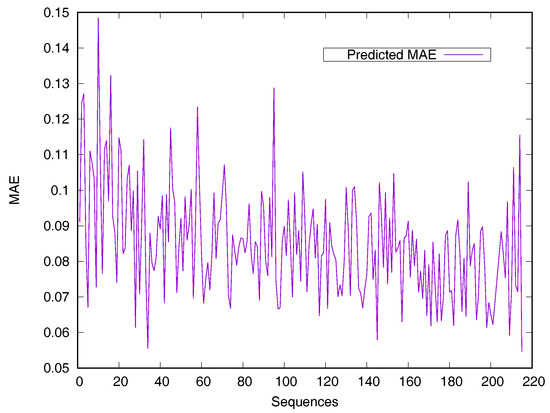
Figure 1.
Predicted MAE based-on individual sequence from the Manesh215 dataset. The protein sequences are ordered by sequence length.
Two publicly-available datasets (CASP10 and CASP11) were also used to validate SDBRNN. CASP10 contains 90 proteins, and CASP11 contains 72 proteins, with the lengths of all sequences between 50 and 600 residues. The PCC value for the CASP10 dataset was 74.2%, which was 3.2% better than that for PredRSA, and that for CASP11 was 74.3%, which was slightly better than SPIDER2 [23].
Another representative method (PSO-SVR [24]) was also compared. The maximum solvent-accessible area standard used in that study was according to Adhamd’s work [10], which used extended tripeptides (Ala-X-Ala). We re-prepared data using the standard and re-trained model. Experiments using our method showed MAE and PCC values of 12.0%, and 0.765, respectively, on the Manesh215 dataset, which were better than 13.2% and 0.74 achieved by PSO-SVR. Additionally, on the CB502 dataset, our method showed MAE and PCC values of 13.3% and 0.739, which were better than 14% and 0.73 obtained by PSO-SVR.
2.3. Comparison of Different Classification Predictors
There are many methods proposed for predicting binary classification (exposed or buried) of residues. Thus, we have also examined the performance of our method in terms of two-state predictions. Similar to the two-layer predictor strategy [37,38], firstly the predicted rASA values were generated by the SDBRNN model. Then, the predicted relative values were transformed into binary states with predefined thresholds for comparison. For instance, the residue with a rASA value that is greater than or equal to the threshold, it can be considered as exposed, otherwise, it is considered as buried. The predictive ability between methods was compared against SARpred [13], PR [29], SVR [28], two-stage SVR [27], SS-SVM [30] and PredRSA using the Manesh215 dataset. Table 3 shows the performances of different methods. Results indicated that the SDBRNN model performed better at RSA prediction and generalization, except for the threshold of 50%.
Table 3.
Binary classification prediction comparison between our method and other reported methods with different thresholds on the Manesh215 dataset.
Predicted accuracy on individual sequence from the Manesh215 dataset is analyzed in Figure 2 for evaluating the model generalization. The prediction accuracy of most proteins is between 75% and 90%. Only 14 sequences out of the 215 proteins have a prediction accuracy of less than 75%.
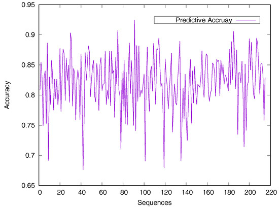
Figure 2.
Predicted accuracy on individual sequences from the Manesh215 dataset. The rASA threshold is 25%. Protein sequences are ordered by sequence length.
We also tested our model using three publicly-available datasets at different thresholds: CB502, Manesh215 and CASP10. ACC and MCC results are listed in Table 4 and Table 5. To compare with PredRSA [22] in detail, its results are also listed in the tables. Our method showed mostly better accuracy on CB502 and Manesh215, except the threshold of 50%. At a threshold of 50%, the ACC associated with the PredRSA on the CB502 and Manesh215 datasets was 0.6% and 0.2% better than our method, respectively. The MCC results of our method are still better than PredRSA.
Table 4.
Accuracy (%) performance comparison in binary classification prediction (the best results are shown in bold).
Table 5.
Matthews’ correlation coefficient performance comparison in binary classification prediction.
2.4. Residue-Specific Variation in Predictive Error
To evaluate the predictive performance for various types of residues, we calculated the average rASA values using the Manesh215 and CB502 datasets for all 20 types of amino acids. SDBRNN accurately predicted RSA using the CB502 dataset with an MAE <1%, except that phenylalanine (F) and tryptophan (W) were predicted with an MAE <1.3% (Figure 3). Most amino acids in the Manesh215 dataset were predicted with an MAE <1%, with tyrosine, histidine, tryptophan and phenylalanine predicted with <2% MAE.
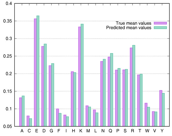
Figure 3.
Comparison of true mean values and predicted mean values for 20 types of amino acids using the CB502 dataset.
3. Discussion
To improve the performance on different combinations of sequence-derived features, we validated five types of input variables using the TR7000 dataset for training and an independent test set (TS261). The performance of the method on different feature combinations was compared, with the results (Table 6) indicating that all five features contributed to RSA prediction.
Table 6.
Different combinations of sequence-derived features for SDBRNN predictors on an independent test set (TS261).
When bidirectional information from a hidden node is merged in the BRNN , concatenation (concat) [51] and sum [47] are commonly used. In the SDBRNN, three merging operators (“concat”, “sum” and “weighting sum”) were used in different hidden layers. To assess the generalization of this BRNN model using hybrid merging operators, we compared the SDBRNN with a BLSTM using the “concat” operator (BLSTM_C), with an BLSTM using the “sum” operator (BLSTM_S) and with a unidirectional LSTM with 800 hidden nodes. Hyperparameters for the BLSTM_C and BLSTM_S were the same as those used for the SDBRNN, and rASA prediction was used to compare the different models. The results listed in Table 7 show that hybrid merging operators effectively promoted better predictive performance.
Table 7.
Comparison of different LSTM models on relative RSA area prediction. MAE is the value percentage (%).
4. Materials and Methods
4.1. Datasets and Input Features
A large, non-homologous sequence dataset, produced using the PISCES server [52], was obtained. Structures exhibited <25% similarity and showed a resolution >3.0 Å, with R factors of 1.0. Three-dimensional structure files were downloaded from the RCSB Protein Data Bank. After removing redundancy in the test datasets using cd-hit [53], 7361 proteins (CullPDB7361) comprising 1,596,728 residues in proteins with sequence lengths between 50 and 600 residues were retained. Among these, 7000 proteins (TR7000) were used for training, and 261 proteins (TS261) and 100 proteins (VD100) were randomly selected for testing and validating the model. In addition to CullPDB7361, three public testing datasets, CB502, Manesh215 and CASP10, were used to evaluate the performance of our model. CB502 (82,420 residues) was selected from CB513 [54] and ordered by sequence length from long to short. The Manesh215 dataset [25] contains 47,243 residues. CASP10 from the Protein Sequence Prediction Center (http://predictioncenter.org/) has 123 domain fragments and extracts from 103 chains. The CASP10 dataset was selected according to protein identity and contained 20,778 residues from 90 proteins. The sequence lengths of the proteins in test datasets were all ≤600.
Five types of features, PSSM, protein sequence coding, conservation score, physical properties and physicochemical characteristics, were used as input features. PSSM-derived features have been widely used to perform protein-related predictions. PSSMs provide the effective frequency of occurrence of all 20 amino acid residues at each position of the sequence. PSSMs can be obtained by performing multiple sequence alignments on a large protein database (NCBI NR database) using PSI-BLAST [55]. PSI-BLAST involves an iterative search process in searching the profile of a query protein. The expectation value (E-value) and the number of iterations for PSI-BLAST are set to 0.001 and three, respectively. The PSSM profile is in the form of a matrix where L is the length and each amino acid in the sequence is described by 20 features.
Physical properties [40] include: a steric parameter (graph-shape index), polarizability, volume (normalized van der Waals volume), hydrophobicity, isoelectric point, helix probability and sheet probability. Specific values were derived from the study [40]. Protein physicochemical characteristics [56] include the number of atoms, electrostatic charges and potential hydrogen bonds.
To ensure smooth transitions in changes to the network gradient, the above features were normalized using a logistic regression function .
Residue conservation was derived from the amino acid frequency distribution in the corresponding column of a multiple-sequence alignment of homologous proteins. A one-dimensional conservation score was computed according to Quan’s [41] previously described Equation (5):
Commonly-used protein coding involves an orthogonal code. In addition to the 20 known residues, “X” represents unknown residues, and “NoSeq” represents non-protein sequences in our coding scheme. A matrix represents a sequence, where L is the sequence length and a 22-dimensional (dim) vector represents a residue in the sequence. However, the 22-dimensional coding vector represents a parsed, one-hot vector, where only one of 22 elements is a non-zero value. For instance, for the residue “A“, the coding is: “1 0 0 0 0 0 0 0 0 0 0 0 0 0 0 0 0 0 0 0 0 0“. We adopted an embedding operation from natural-language processing to transform sparse sequence features into denser representations. This embedding operation was implemented as a simple auto-encoder (a feed-forward neural-network layer) along with an embedding matrix mapping a sparse 22-dimensional vector into a denser 22-dimensional vector. This transformation was just converted into a one-hot vector, which coded one residue into a dense vector.
In our scheme, an input residue was represented by 53-dimensional features: 20-dim PSSM, 7-dimensional physical properties, 3-dimensional physicochemical characteristics, 1-dimensional conservation score and 22-dimensional protein codings. These features are all derived from the protein sequence.
The rASA of a residue in a protein chain is calculated by dividing the accessible surface area derived from DSSP [44] by the maximum solvent accessibility. However, there is no standard for maximum solvent accessibility. According to previous results [22,25], Gly-X-Gly extended tripeptides were used.
4.2. BRNN and Merging Operator
For sequence data , where is context dependent and strongly reliant on forward and backward information. The label vector is the target output space. Compared to a forward neural network, the current output from the recurrent neural network will be reverted backward for subsequent time-specific inputs. The recurrent neural network structure can be described as Equation (6):
At the time , the recurrent network can remember the information from previous and the present input . However, in many applications, the output might be dependent on the entire input sequence, as in protein sequences and handwriting-recognition examples. BRNN [57] combines an RNN that moves forward through time beginning from the start of the sequence along with another RNN that moves backward through time beginning from the end of the sequence. In this BRNN, time-increasing input is represented by , and time-decreasing input is represented by . Bidirectional information is merged as the current node’s output. Therefore, BRNN is more suitable for context-related applications, and it is capable of outperforming unidirectional recurrent neural network. The BRNN can be described as Equation (7):
The BRNN structure is capable of efficiently learning sequence information [45]. Previous studies focused primarily on the BRNN methodology with little research on incorporating bidirectional-information merging. In a conventional neural network, pooling operations are computationally important, with the pooling layer responsible for accumulating convolutional results. The merging operator in a BRNN acts similarly to pooling operations. At time , input forwarded to the current node is represented by , and the backward input is represented by . Therefore, a common formula for the output of the current node is presented in Figure 4 and as follows:
where is the merging operator, . ⨂ represents element-wise multiplication; + is the sum; ⨁ is the element-wise weighting sum; ∞ is concatenation; and ⨀ is the reshape operator. The merging operator can perform more computations than necessary when the information is merged via the aggregation operation.
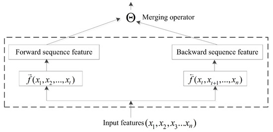
Figure 4.
In order to remember more long-range information in the sequence study, when the past computing information and the future computing information are merged, the merging operator is proposed to execute the merging operation.
4.3. Model
4.3.1. SDBRNN
Protein primary structure represents a strongly time-ordered conformation, suggesting that it contains adequate information for the protein to fold into its native conformation. To capture more features in the primary structure, we use three types of computing operators in the merging operation. During the initial period, the computing node in the BRNN needs to remember backward, forward and current input information; therefore, the merging operator “concat” is used in the first layer. In the second layer, the computing node no longer needs to remember previous and future information; however, the “sum” operator reinforces bidirectional input aggregation, with bidirectional information again aggregated in the third layer. Therefore, a “weighting sum” operator is used for filtering unnecessary information and extracting key features. The equations associated with these operations are as follows (9)–(11):
The recurrent neural network accepts a time-stepping sequence that makes the network extremely deep, with the depth making the network difficult to train because of the exploding or vanishing gradient [46]. Long short-term memory (LSTM) [58], which consists of a variety of gate structures (a forget gate, an input gate and an output gate) and a memory cell are used to address the vanishing gradient problem. In the SDBRNN architecture, the unidirectional computing node is performed by LSTM. The widely-accepted LSTM definition was provided by Graves [59], and the details of LSTM are described in Equation (12), which involves no peep-hole connections, mainly to improve computing performance.
where is the sigmoid function; and c are respectively the input gate, forget gate, output gate and cell activation vectors, all of which are the same size as the hidden vector h.
The following BRNN layer represents a multi-layer perceptron (MLP) network that reduces the network scale. The MLP layer with logistic activation ultimately outputs the prediction, with logistic regression used for fitting the relative surface-area value. The SDBRNN architecture is shown in Figure 5. The cross-entropy loss function is used for model training:
where are the predicted probabilities of secondary structure labels, represent ground-truth labels of the secondary structure and N is the number of input residues. is a vector of output activations prior to normalization with the logistic function. These derivatives are then fed back through the network using back propagation through time to determine the weight gradient.
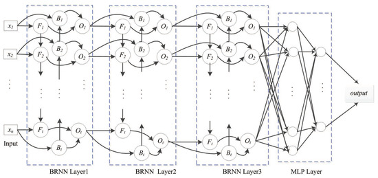
Figure 5.
SDBRNN architecture. The merging operator “concat” is used in the first BRNN layer. The “sum” and “weighting sum” operator are used in the second and third layer. Two multi-perception networks are connected to BRNN.
In our model, rASA prediction is simulated as a regressive problem. With the predicted rASA values, the classifications are carried out in two states (buried and exposed). We have tried seven thresholds of 5, 10, 20, 25, 30, 40 and 50% in the two-state classification.
4.3.2. Model Hyperparameters
SDBRNNs have three BRNN layers and two MLP layers. The first BRNN layer has 300 nodes, with 500 nodes in the other two layers. The first MLP layer has 128 nodes, and the second has 60 nodes. The Adam optimizing function was used for training the network using default settings, with the default learning rate set to 0.0008. This was reduced by 50%, whereas the validation accuracy decreased by more than 10-times. The threshold of the learning rate was set to 0.0001.
A natural stopping policy was accepted while the validation stopped decreasing. To balance model performance between fitting and generalization, a regularization or penalty term was attached to the loss function (e.g., or ). Unlike other models, regularization was not attached, and our experiment displayed dropout efficiency [60]. Except for the classification layer, each layer was regularized according to a dropout (p = 0.5) to avoid overfitting. Our model was implemented in Keras, which is a public deep learning software based on Theano [61]. Weights in the SDBRNN were initialized with default values in Keras. The network was trained using a single NVIDIA Tesla K40 GPU with 12 GB memory. Training the model requires about 16.5 min per epoch, and it takes about 0.04 seconds to test one sequence.
Proteins shorter than 600 AA were padded with all-zero features. The outputs corresponding to padded inputs are labeled as 0.5 according to the logistic function. The advantage of padding proteins is that it enables training the model on a GPU in batches.
5. Conclusions
Accessible RSA is often used as an important measure in proteomics study for describing protein properties. Compared with traditional machine learning techniques, deep learning exhibits wider generalization and is applied in our study to predict RSA area. Deep neural networks are stacked by various complicated neural networks, and more generalized representation capacity can be obtained. However, the deep neural networks own enormous parameters and need more samples and computing resources to train models. Use of the merging operator was proposed for merging computations in the BRNN hidden layer. We redesigned BLSTM merging using three types of merging operators (“concat”, “sum”, and “weighting sum”) in SDBRNN. Compared with the commonly-used BLSTM method using a single merging operator, as well as other predictors, SDBRNN captured more protein features and was more generalizable. Our results on test datasets verified this.
Relative solvent-accessible areas are greatly affected by maximum solvent-accessible areas, as more maximum solvent-accessible areas will lead to lower relative solvent-accessible areas and lower MAEs. However, there are no standard maximum solvent accessible areas. In this work, a novel deep learning method (SDBRNN) was presented for the prediction of RSA area, as well as for binary state classification. Our methods can be applied to a broad range of problems within and outside of computational biology.
Supplementary Materials
The following are available online at http://www.mdpi.com/2218-273X/8/2/33/s1, File f1: PDB-ID list of CullPDB7361. Table t1: Predicted MAE and accuracy at the threshold of 25% of individual sequences on the Manesh215 dataset.
Author Contributions
Q.L. conceived of the study. B.Z. performed the experiments, analyzed the data and initially drafted the manuscript. L.L. collected the features. All authors contributed to the revision and approved the final manuscript.
Funding
This research was funded by National Natural Science Foundation of China grant number No. 61170125, the Special Program for Applied Research on Super Computation of the NSFC-Guangdong Joint Fund (the second phase) and the Natural Science Research Project of Anhui Provincial Department of Education grant number No. KJ2018A0383.
Acknowledgments
Our thanks are given to the reviewers for their helpful suggestions.
Conflicts of Interest
The authors declare no conflict of interest.
Abbreviations
The following abbreviations are used in this manuscript:
| RSA | Residue Solvent Accessibility |
| rASA | relative accessible solvent area |
| BLSTM | bidirectional long-short memory |
| SDBRNN | stacked deep bidirectional recurrent neural network |
| RNN | recurrent neural network |
| BRNN | bidirectional recurrent neural network |
| LSTM | long short-term memory |
| MLP | multi-layer perceptron |
| MAE | mean absolute error |
| PCC | Pearson’s correlation coefficient |
| MCC | Matthews’ correlation coefficient |
| ACC | Accuracy |
References
- Lee, B.; Richards, F.M. The interpretation of protein structures: Estimation of static accessibility. J. Mol. Biol. 1971, 55, 379–400. [Google Scholar] [CrossRef]
- Rost, B.; Sander, C. Conservation and prediction of solvent accessibility in protein families. Proteins Struct. Funct. Bioinform. 1994, 20, 216–226. [Google Scholar] [CrossRef] [PubMed]
- Wodak, S.J.; Janin, J. Location of structural domains in protein. Biochemistry 1981, 20, 6544–6552. [Google Scholar] [CrossRef] [PubMed]
- Liu, S.; Zhang, C.; Liang, S.; Zhou, Y. Fold recognition by concurrent use of solvent accessibility and residue depth. Proteins Struct. Funct. Bioinform. 2007, 68, 636–645. [Google Scholar] [CrossRef] [PubMed]
- Mooney, C.; Pollastri, G.; Shields, D.C.; Haslam, N.J. Prediction of short linear protein binding regions. J. Mol. Biol. 2012, 415, 193–204. [Google Scholar] [CrossRef] [PubMed]
- Connolly, M.L. Solvent-accessible surfaces of proteins and nucleic acids. Science 1983, 221, 709–713. [Google Scholar] [CrossRef] [PubMed]
- Huang, B.; Schroeder, M. LIGSITE csc: Predicting ligand binding sites using the Connolly surface and degree of conservation. BMC Struct. Biol. 2006, 6, 19. [Google Scholar] [CrossRef] [PubMed]
- Janin, J. Surface and inside volumes in globular proteins. Nature 1979, 277, 491. [Google Scholar] [CrossRef] [PubMed]
- Rose, G.; Geselowitz, A.; Lesser, G.; Lee, R.; Zehfus, M. Hydrophobicity of amino acid residues in globular proteins. Science 1985, 229, 834–838. [Google Scholar] [CrossRef] [PubMed]
- Ahmad, S.; Gromiha, M.M.; Sarai, A. Real value prediction of solvent accessibility from amino acid sequence. Proteins Struct. Funct. Bioinform. 2003, 50, 629–635. [Google Scholar] [CrossRef] [PubMed]
- Holbrook, S.R.; Muskal, S.M.; Kim, S.H. Predicting surface exposure of amino acids from protein sequence. Protein Eng. 1990, 3, 659–665. [Google Scholar] [CrossRef] [PubMed]
- Ahmad, S.; Gromiha, M.M. NETASA: Neural network based prediction of solvent accessibility. Bioinformatics 2002, 18, 819–824. [Google Scholar] [CrossRef] [PubMed]
- Garg, A.; Kaur, H.; Raghava, G.P. Real value prediction of solvent accessibility in proteins using multiple sequence alignment and secondary structure. Proteins Struct. Funct. Bioinform. 2005, 61, 318–324. [Google Scholar] [CrossRef] [PubMed]
- Dor, O.; Zhou, Y. Real-SPINE: An integrated system of neural networks for real-value prediction of protein structural properties. Proteins Struct. Funct. Bioinform. 2007, 68, 76–81. [Google Scholar] [CrossRef] [PubMed]
- Faraggi, E.; Xue, B.; Zhou, Y. Improving the prediction accuracy of residue solvent accessibility and real-value backbone torsion angles of proteins by guided-learning through a two-layer neural network. Proteins Struct. Funct. Bioinform. 2009, 74, 847–856. [Google Scholar] [CrossRef] [PubMed]
- Kim, H.; Park, H. Prediction of protein relative solvent accessibility with support vector machines and long-range interaction 3D local descriptor. Proteins Struct. Funct. Bioinform. 2004, 54, 557–562. [Google Scholar] [CrossRef] [PubMed]
- Wang, J.Y.; Lee, H.M.; Ahmad, S. SVM-Cabins: Prediction of solvent accessibility using accumulation cutoff set and support vector machine. Proteins Struct. Funct. Bioinform. 2007, 68, 82–91. [Google Scholar] [CrossRef] [PubMed]
- Wang, J.Y.; Lee, H.M.; Ahmad, S. Prediction and evolutionary information analysis of protein solvent accessibility using multiple linear regression. Proteins Struct. Funct. Bioinform. 2005, 61, 481–491. [Google Scholar] [CrossRef] [PubMed]
- Thompson, M.J.; Goldstein, R.A. Predicting solvent accessibility: Higher accuracy using Bayesian statistics and optimized residue substitution classes. Proteins Struct. Funct. Bioinform. 1996, 25, 38. [Google Scholar] [CrossRef]
- Joo, K.; Lee, S.J.; Lee, J. Sann: Solvent accessibility prediction of proteins by nearest neighbor method. Proteins Struct. Funct. Bioinform. 2012, 80, 1791. [Google Scholar] [CrossRef] [PubMed]
- Iqbal, S.; Mishra, A.; Hoque, M.T. Improved prediction of accessible surface area results in efficient energy function application. J. Theor. Biol. 2015, 380, 380–391. [Google Scholar] [CrossRef] [PubMed]
- Fan, C.; Liu, D.; Huang, R.; Chen, Z.; Deng, L. PredRSA: A gradient boosted regression trees approach for predicting protein solvent accessibility. BMC Bioinform. 2016, 17, S8. [Google Scholar] [CrossRef] [PubMed]
- Heffernan, R.; Paliwal, K.; Lyons, J.; Dehzangi, A.; Sharma, A.; Wang, J.; Sattar, A.; Yang, Y.; Zhou, Y. Improving prediction of secondary structure, local backbone angles, and solvent accessible surface area of proteins by iterative deep learning. Sci. Rep. 2015, 5, 11476. [Google Scholar] [CrossRef] [PubMed]
- Zhang, J.; Chen, W.; Sun, P.; Zhao, X.; Ma, Z. Prediction of protein solvent accessibility using PSO-SVR with multiple sequence-derived features and weighted sliding window scheme. BioData Min. 2015, 8, 3. [Google Scholar] [CrossRef] [PubMed]
- Naderi-Manesh, H.; Sadeghi, M.; Arab, S.; Moosavi Movahedi, A.A. Prediction of protein surface accessibility with information theory. Proteins 2001, 42, 452–459. [Google Scholar] [CrossRef]
- Nepal, R.; Spencer, J.; Bhogal, G.; Nedunuri, A.; Poelman, T.; Kamath, T.; Chung, E.; Kantardjieff, K.; Gottlieb, A.; Lustig, B. Logistic regression models to predict solvent accessible residues using sequence- and homology-based qualitative and quantitative descriptors applied to a domain-complete X-ray structure learning set. J. Appl. Crystallogr. 2015, 48, 1976–1984. [Google Scholar] [CrossRef] [PubMed]
- Nguyen, M.N.; Rajapakse, J.C. Prediction of protein relative solvent accessibility with a two-stage SVM approach. Proteins Struct. Funct. Bioinform. 2005, 59, 30–37. [Google Scholar] [CrossRef] [PubMed]
- Chang, D.T.; Huang, H.Y.; Syu, Y.T.; Wu, C.P. Real value prediction of protein solvent accessibility using enhanced PSSM features. BMC Bioinformat. 2008, 9, 1–12. [Google Scholar] [CrossRef] [PubMed]
- Meshkin, A.; Sadeghi, M.; Ghasem-Aghaee, N. Prediction of relative solvent accessibility using pace regression. EXCLI J. 2009, 8, 211–217. [Google Scholar]
- Kashefi, A.H.; Meshkin, A.; Zargoosh, M.; Zahiri, J.; Taheri, M.; Ashtiani, S. Scatter-search with support vector machine for prediction of relative solvent accessibility. Excli J. 2013, 12, 52–63. [Google Scholar] [PubMed]
- Qian, N.; Sejnowski, T.J. Predicting the secondary structure of globular proteins using neural network models. J. Mol. Biol. 1988, 202, 865–884. [Google Scholar] [CrossRef]
- Rost, B.; Sander, C. Improved prediction of protein secondary structure by use of sequence profiles and neural networks. Proc. Natl. Acad. Sci. USA 1993, 90, 7558–7562. [Google Scholar] [CrossRef] [PubMed]
- Wan, S.; Mak, M.W.; Kung, S.Y. Transductive Learning for Multi-Label Protein Subchloroplast Localization Prediction. IEEE/ACM Trans. Comput. Biol. Bioinform. 2016, 14, 212–224. [Google Scholar] [CrossRef] [PubMed]
- Chou, K.C.; Shen, H.B. Cell-PLoc: A package of Web servers for predicting subcellular localization of proteins in various organisms. Nat. Protoc. 2008, 3, 153–162. [Google Scholar] [CrossRef] [PubMed]
- Wan, S.; Mak, M.W.; Kung, S.Y. FUEL-mLoc: Feature-unified prediction and explanation of multi-localization of cellular proteins in multiple organisms. Bioinformatics 2017, 33, 749–750. [Google Scholar] [CrossRef] [PubMed]
- Hayat, M.; Khan, A. MemHyb: Predicting membrane protein types by hybridizing SAAC and PSSM. J. Theor. Biol. 2012, 292, 93. [Google Scholar] [CrossRef] [PubMed]
- Chou, K.C.; Shen, H.B. MemType-2L: A web server for predicting membrane proteins and their types by incorporating evolution information through Pse-PSSM. Biochem. Biophys. Res. Commun. 2007, 360, 339–345. [Google Scholar] [CrossRef] [PubMed]
- Wan, S.; Mak, M.W.; Kung, S.Y. Mem-ADSVM: A two-layer multi-label predictor for identifying multi-functional types of membrane proteins. J. Theor. Biol. 2016, 398, 32–42. [Google Scholar] [CrossRef] [PubMed]
- Wan, S.; Mak, M.W.; Kung, S.Y. Ensemble linear neighborhood propagation for predicting subchloroplast localization of multi-location proteins. J. Proteome Res. 2016, 15, 4755–4762. [Google Scholar] [CrossRef] [PubMed]
- Meiler, J.; Müllerl, M.; Zeidler, A.; Schmäschke, F. Generation and evaluation of dimension-reduced amino acid parameter representations by artificial neural networks. J. Mol. Model. 2001, 7, 360–369. [Google Scholar] [CrossRef]
- Quan, L.; Lv, Q.; Zhang, Y. STRUM: Structure-based prediction of protein stability changes upon single-point mutation. Bioinformatics 2016, 32, 2936. [Google Scholar] [CrossRef] [PubMed]
- Bowie, J.U.; Luthy, R.; Eisenberg, D. A Method to Identify Protein Sequences that Fold into a Known Three- Dimensional Structure. Science 1991, 253, 164. [Google Scholar] [CrossRef] [PubMed]
- Wu, W.; Wang, Z.; Cong, P.; Li, T. Accurate prediction of protein relative solvent accessibility using a balanced model. Biodata Min. 2017, 10, 1. [Google Scholar] [CrossRef] [PubMed]
- Kabsch, W.; Sander, C. Dictionary of protein secondary structure: Pattern recognition of hydrogen-bonded and geometrical features. Biopolymers 1983, 22, 2577–2637. [Google Scholar] [CrossRef] [PubMed]
- Lecun, Y.; Bengio, Y.; Hinton, G. Deep learning. Nature 2015, 521, 436–444. [Google Scholar] [CrossRef] [PubMed]
- Jozefowicz, R.; Zaremba, W.; Sutskever, I. An Empirical Exploration of Recurrent Network Architectures. In Proceedings of the 32nd International Conference on Machine Learning (ICML), Lille, France, 6–11 July 2015; pp. 171–180. [Google Scholar]
- Li, Z.; Yu, Y. Protein Secondary Structure Prediction Using Cascaded Convolutional and Recurrent Neural Networks. In Proceedings of the 25th International Joint Conference on Artificial Intelligence(IJCAI), New York, NY, USA, 9–15 July 2016; pp. 2560–2567. [Google Scholar]
- Wan, F.; Zeng, J. Deep learning with feature embedding for compound-protein interaction prediction. bioRxiv 2016. [Google Scholar] [CrossRef]
- Zhou, J.; Troyanskaya, O.G. Deep Supervised and Convolutional Generative Stochastic Network for Protein Secondary Structure Prediction. In Proceedings of the 31st International Converenfe on Machine Learning (ICML), Beijing, China, 21–26 June 2014; pp. 745–753. [Google Scholar]
- Petersen, B.; Petersen, T.N.; Andersen, P.; Nielsen, M.; Lundegaard, C. A generic method for assignment of reliability scores applied to solvent accessibility predictions. BMC Struct. Biol. 2009, 9, 51. [Google Scholar] [CrossRef] [PubMed]
- Chen, J.; Chaudhari, N.S. Cascaded Bidirectional Recurrent Neural Networks for Protein Secondary Structure Prediction. IEEE/ACM Trans. Comput. Biol. Bioinform. 2007, 4, 572–582. [Google Scholar] [CrossRef] [PubMed]
- Wang, G.; Dunbrack, R.L., Jr. PISCES: A protein sequence culling server. Bioinformatics 2003, 19, 1589–1591. [Google Scholar] [CrossRef] [PubMed]
- Li, W.; Godzik, A. Cd-hit: A fast program for clustering and comparing large sets of protein or nucleotide sequences. Bioinformatics 2006, 22, 1658. [Google Scholar] [CrossRef] [PubMed]
- Cuff, J.; Barton, G. Application of multiple sequence alignment profiles to improve protein secondary structure prediction. Proteins 2000, 40, 502–511. [Google Scholar] [CrossRef]
- Altschul, S.F.; Gertz, E.M.; Agarwala, R.; Schaäffer, A.A.; Yu, Y.K. PSI-BLAST pseudocounts and the minimum description length principle. Nucleic Acids Res. 2009, 37, 815–824. [Google Scholar] [CrossRef] [PubMed]
- Nan, L.; Zhonghua, S.; Fan, J. Prediction of protein-protein binding site by using core interface residue and support vector machine. BMC Bioinform. 2009, 9, 553. [Google Scholar]
- Schuster, M.; Paliwal, K.K. Bidirectional recurrent neural networks. IEEE Trans. Signal Process. 1997, 45, 2673–2681. [Google Scholar] [CrossRef]
- Hochreiter, S.; Schmidhuber, J. Long Short-Term Memory. Neural Comput. 1997, 9, 1735. [Google Scholar] [CrossRef] [PubMed]
- Graves, A.; Jaitly, N.; Mohamed, A.R. Hybrid speech recognition with Deep Bidirectional LSTM. In Proceedings of the Automatic Speech Recognition and Understanding, Olomouc, Czech Republic, 8–12 December 2014; pp. 273–278. [Google Scholar]
- Srivastava, N.; Hinton, G.; Krizhevsky, A.; Sutskever, I.; Salakhutdinov, R. Dropout: A simple way to prevent neural networks from overfitting. J. Mach. Learn. Res. 2014, 15, 1929–1958. [Google Scholar]
- Theano Development Team. Theano: A Python framework for fast computation of mathematical expressions. arXiv, 2016; arXiv:1605.02688. [Google Scholar]


© 2018 by the authors. Licensee MDPI, Basel, Switzerland. This article is an open access article distributed under the terms and conditions of the Creative Commons Attribution (CC BY) license (http://creativecommons.org/licenses/by/4.0/).