Constrained Molecular Dynamic Simulation of the Potential Mean Force of Lithium Bromide Ion Pairs in Acetonitrile

Abstract

Molecular dynamic simulations of Li⁺, and Br⁻ ions in acetonitrile were carried out. The simulated structural properties were compared to experimental data. The solvent potentials of Li⁺-Br⁻, Li⁺-Li⁺, and Br⁻-Br⁻ were evaluated using constrained molecular dynamics (CMD) simulations, to determine the solvent contribution to the total force acting on the solute and estimate the liquid arrangements according to the potential of mean force (PMF) values. The PMF of friction kernels and the passage across the Li⁺-Br⁻ barrier was studied using the Grote–Hynes theory. The union-separation development happens in the polarization confining system.

1. Introduction

Understanding ionic association in polar solvents at the molecular level is vital to interpreting many chemical and biological processes [1]. Much research is being carried out based on molecular dynamics simulations of ionic liquids in polar diluents, such as methanol and water [2,3,4]. Constrained molecular dynamics (CMD) [5] simulations are performed while maintaining a fixed interior separation. In this way, the ion–ion potential of mean force (PMF) and coefficients of relative friction can be obtained to determine the association constants. In addition, such simulations can reveal the behavior of ions and adjacent molecules at the microscopic level. A characteristic of the liquids mentioned is that, unlike acetonitrile (MeCN), they form hydrogen bridges.

Equations for deriving PMF values for lithium bromide in acetonitrile through simulations have not yet been established, although theoretical calculations can be performed via the Ornstein–Zernike equation using a hypernetted-chain (HNC) approach [6]. Acetonitrile is a widely used organic solvent whose molecules do not form hydrogen bonds, unlike water (H₂O) and methanol (MeOH). In addition, it has a relative permittivity (${\epsilon }_r^{\mathrm{MeCN}}=36$) significantly lower than that of water (${\epsilon }_r^{{\mathrm{H}}_2\mathrm{O}}=78$) and similar to that of methanol (${\epsilon }_r^{\mathrm{MeOH}}=34$). It can be beneficial to compare the results obtained with different solvents. The ion pair (Li⁺-Br⁻) was chosen in this study because data on neutron diffraction [7] and dielectric relaxation [8] are available for comparison. In the last 20 years, a great deal of progress has been made in the study of ions in solution (both aqueous and non-, and both experimental and theoretical). For example, the importance of explicit polarizability in models to describe solvation of anions such as Br⁻ is well established, and certainly new experimental data using neutron scattering or other methods are available. Metal salt solutions in polar aprotic solvents have a wide range of uses, including electrolytes in electrochemical devices (such as lithium batteries with high energy density, capacitors, and so on) and reagents in organometallic chemistry. The details of interactions between dissolved salt ions and organic solvent molecules influence the density, viscosity, volatility, ionic conductivity, and other essential properties of ionic solutions. As a result, ion–solvent interactions appear to be critical for furthering our understanding of ionic solutions. The interaction of solvents with positive and negative ions differs significantly, making it difficult to obtain a thorough knowledge of the anion solvation mechanism. Because of the huge size of anions, their intricate geometry (for polyatomic anions) and charge distribution, anion solvent interactions are weaker than cation solvent interactions. Second, in aprotic solvents, anion solvation is mostly accomplished through hydrogen bonding, which is absent in anionic solvents. For these reasons, it is commonly assumed that metal salt dissolving in polar aprotic solvents occurs solely due to the solvation of metal cations, whereas anions remain uncoordinated by the solvent molecules. Nevertheless, a thorough investigation of monoatomic halide anions using both theoretical and experimental methods has revealed that these notions are oversimplified, and that interactions of the halide anion with polar aprotic solvent molecules is possible. The weak halide–solvent interactions, on the other hand, make theoretical analyses of halide solvation difficult, necessitating a fine balance between ion–solvent and solvent–solvent interactions. For bromide, as well as aprotic and non-polar solvents, this trend becomes very pronounced. When acetonitrile is utilized as the solvent, solvation numbers in the range of 1–9 are discovered in the literature for this anion. Furthermore, the solvent molecules’ molecular organization is not well understood [9,10,11].

The PMF values (W (r)) between particles with electrical charge in liquid perform a crucial part of the analysis of liquefied mixtures. CMD, as a computer simulation technique, is very useful for calculating W (r). CMD simulations can be used to calculate the mean force (MF) exerted on dissolved substance by solvent, whereas the separation between the solute is constrained. We used CMD and non-constrained (non-CMD) simulations to calculate the W(r) of Li⁺-Br⁻, Li⁺-Li⁺, and Br⁻-Br⁻ and the dynamics of these particles with electrical charge.

This article is structured as follows. Details of our simulations and interaction potential models are given in Section 2. The ion–solvent structural properties obtained from the non-CMD simulations, the ion–ion MF along with PMF results obtained for all the simulations and the Li⁺-Br⁻ pair friction kernel and the interconversion process are analyzed in Section 3. The conclusions of this paper are summarized in Section 4.

2. Materials and Methods

The PMF values for Li⁺-Br⁻, Li⁺-Li⁺, and Br⁻-Br⁻ in acetonitrile have been evaluated. We carried out CMD simulations of systems built of two ions and 214 solvent molecules located in a cubic box with periodic boundary conditions. The volume of the cubic box (L = 26.58 Å) was selected to give a solvent density of 0.777 g/cm³ and with a temperature of 298 K. Additionally, non-CMD simulations were performed for two systems with free ions: one with Li⁺ and another with Br⁻. All code/programs-software used to perform the simulations were developed in-house. Mainly the simulations codes were developed using Fortran 77. The code included routines which evaluated the interaction potential, periodic conditions, integration algorithms, implementation of constraints (SHAKE procedure) and the mean force. See the Appendix A and Appendix B for simulation details.

We used an “acetonitrile rigid molecule pairwise additive potential model” [12,13] and performed calculations for the nitrogen (N), carbon (C) and methyl group (Me) interaction sites. Me is considered to be a unit atom model. The methyl-carbon and carbon-nitrogen distances were 1.458 Å and 1.157 Å, respectively, as shown in Figure 1. The dipole moment of each acetonitrile molecule is equal to 3.96 D.

The ion–ion, ion–solvent and solvent–solvent interactions were evaluated using the following mathematical expression:

$$W_{mn}={{\displaystyle \sum }}_i^{on m}{{\displaystyle \sum }}_j^{on n}\left(\frac{A_i{A}_j}{r_{ij}^{12}}-\frac{C_i{C}_j}{r_{ij}^6}+\frac{q_i{q}_j}{r_{ij}}\right),$$

(1)

in terms of the Lennard–Jones parameters, $A_i^2=4{\epsilon }_i{\sigma }_i^{12}$, $C_i^2=4{\epsilon }_i{\sigma }_i^6$ and $q_i$ is the charge allocated to the place i.

We used the parameters for Li⁺ and Br⁻ derived by Chandrasekhar et al. [14] and Lybrand [15] from first principles computations of free ions in ${\mathrm{H}}_2\mathrm{O}$. The values of the parameters are summarized in

Table 1. Lennard–Jones Interaction potential parameters.

Atom/Ion	ε/kcal mol−1	σ/Å	q/e
a Me	0.1869	3.775	+0.206
a C	0.130	3.650	+0.247
a N	0.15	3.200	−0.453
b Li+	6.25	1.26	+1.0
c Br−	0.0907	4.62	−1.0

^a Values from [12]. ^b Values from [14]. ^c Values from [15].

. By using the same ion’s Lennard–Jones parameters for acetonitrile as for water, we are assuming that ε and σ transfer from one solvent to another.

Table 2. Range of inter ion distances and total number of CMD simulations conducted for each ion pair.

Ion Pair	${\mathit{r}}_{\mathit{m}\mathit{i}\mathit{n}}-{\mathit{r}}_{\mathit{m}\mathit{a}\mathit{x}}$	No. of Simulations
Li+-Br−	1.8 Å–9.0 Å	37
Li+-Li+	2.0 Å–9.0 Å	36
Br−-Br−	4.0 Å–9.0 Å	26

summarizes the range of the interionic separation for each pair and the total number of simulations performed. Each simulation consisted of a stabilization interval of 25 ps followed by a generation time of 50 ps. For certain interionic separations, CMD simulations of 100 ps were carried out to calculate statistical errors and friction kernels, and for detailed study of the configuration of the solvent over the ion pairs. In the case of acetonitrile, an integration step of 0.005 ps was used. We used the integration algorithm of Berendsen et al. [16] with the SHAKE technique [17] to fix the molecular distances. The Lennard–Jones interactions were cut off at L/2 and the long-range exchanges were calculated by the Ewald sum technique [18].

Radial distribution functions $(g\left(r\right))$. The number of particles in a volume dr centered at r, provided that one is at the origin is $N\left(r+dr\right) = {\rho }_{bulk}·g\left(r\right)·dr$; we know that $(g\left(r\right))$ depends solely on the modulus r, so we may better consider the number of particles contained in a spherical shell of radius r and r + Δr, given by $N\left(r,r+\mathsf{\Delta }r\right) = 4\pi ·{\rho }_{bulk}·r^2·g\left(r\right)·\mathsf{\Delta }r$, from this formula $g\left(r\right)$ can be calculated as, $g\left(r\right) = \underset{\mathsf{\Delta }r\to 0}{\lim }\frac{N\left(r,r+\mathsf{\Delta }r\right)}{4\pi ·{\rho }_{bulk}·r^2·\mathsf{\Delta }r}$.

In a practical simulation, a finite Δr is considered. At each time step of the numerical integration, all the pairs separated by a distance (r, r + Δr) would be counted and added to a histogram, then a coarse-grained g(r) is obtained.

Finally, we carried out two unconstrained simulations of Li⁺ and Br⁻, with 215 solvent molecules. The information obtained from these ion–solvent structure simulations is compared to the neutron diffraction data in Section 3. In addition, these simulations are representative of an infinitely diluted solution (zero concentration limit). According to Chandrasekhar and Jorgensen [19], the enthalpy of dissolution ($\mathsf{\Delta }{H}_{sol}$) can be determined from these simulations by means of the following expression:

$$\mathsf{\Delta }{H}_{sol}=\mathsf{\Delta }{U}_{sol}+P\mathsf{\Delta }{V}_{sol}-R{T}_{ref},$$

(2)

where the last two terms are negligible under normal environmental conditions, and $\mathsf{\Delta }{U}_{sol}$ is the difference between the interaction energy of the infinite dilution system $(U_{sol}^{\infty })$ and the pure solvent ($U{ }^{*}$):

$$\mathsf{\Delta }{U}_{sol}=U_{sol}^{\infty }-U^{*},$$

(3)

although these expressions are commonly used to determine $\mathsf{\Delta }{H}_{sol}$ from the simulations, we will use them in reverse to obtain an experimental estimate of $U_{sol}^{\infty }$ from the experimental results of $\mathsf{\Delta }{H}_{sol}$ and U*.

Table 3. Comparison between the experimental and simulation results regarding the interaction energy of a solution at infinite dilution $U_{sol}^{\infty }\left(\mathrm{kcal} \mathrm{mo}{\mathrm{l}}^{-1}\right)$.

Ion	$\mathbf{\Delta }{\mathit{H}}_{\mathit{s}\mathit{o}\mathit{l}}\left(\mathit{e}\mathit{x}\mathit{p}\right)$	${\mathit{U}}^{*}/\mathit{N} \left(\mathit{e}\mathit{x}\mathit{p}\right)$	${\mathit{U}}_{\mathit{s}\mathit{o}\mathit{l}}^{\mathit{\infty }}\left(\mathit{N}+1\right)\left(\mathit{e}\mathit{x}\mathit{p}\right)$	${\mathit{U}}_{\mathit{s}\mathit{o}\mathit{l}}^{\mathit{\infty }}\left(\mathit{N}+1\right)\left(\mathit{s}\mathit{i}\mathit{m}\right)$
Li+		−7.4 b		−7.48
Br−	−80 a		−7.73	−7.11

^a from Ref. [20]; ^b from Ref. [21].

shows the $U_{sol}^{\infty }$ values corresponding to our simulations, which are compared against the experimental values obtained from the procedure described above.

3. Results and Discussion

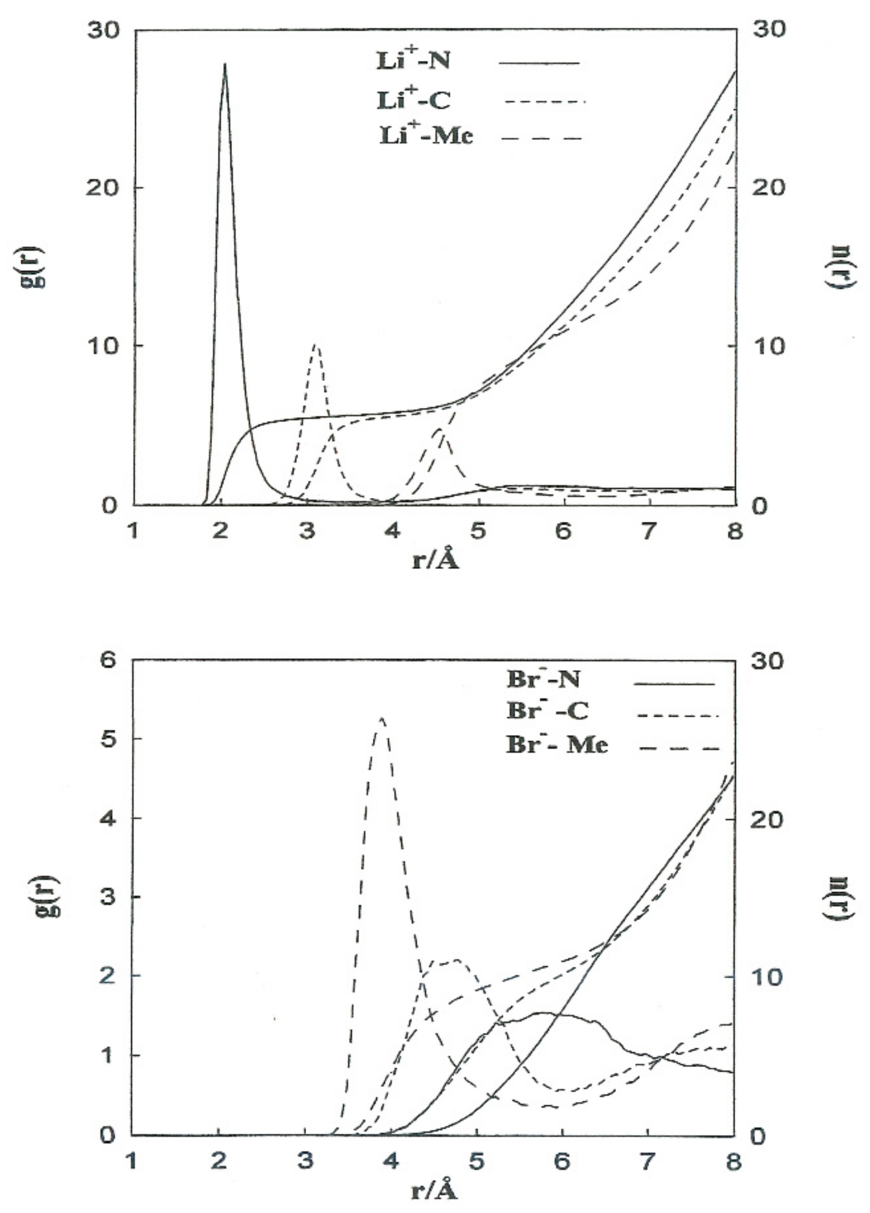
3.1. Ion–Acetonitrile Structural Properties

The structural properties obtained from the non-CMD simulations of Li⁺ and Br⁻ ions in acetonitrile are shown in Figure 2 (left axis) in the form of ion-acetonitrile radial distribution functions $\left[g_{I\mathrm{MeCN}}\left(r\right) = g_{I\mathrm{N}}\left(r\right), g_{I\mathrm{C}}\left(r\right),g_{I\mathrm{Me}}\left(r\right)\right]$. We similarly calculated the running coordination numbers ($n\left(r\right)$) which is giving by $n\left(r\right) = 4\pi \rho {{\displaystyle \int }}_0^r{r^{\prime }}^{2}g\left(r^{\prime }\right)d{r}^{\prime }$ where $\rho$ is the numeric solvent density. The function $n\left(r\right)$ gives the mean number of molecules within a sphere of radius r centered on the ion. The coordination number is defined as the plateau value of $n\left(r\right)$ at distances close to the first g(r) minimum (Figure 2, right axis).

Table 4. Ion-atom distances and corresponding coordination numbers.

Atoms	Distance/Å		Coordination Number
	Simulation	Experiment a	Simulation	Experiment a
Li+-N	2.025	2.05	5.5	$2.9\pm 0.3$
Li+-C	3.075	3.17	5.5	$3.4\pm 0.3$

Source: ^a from Ref. [7].

summarizes the positions of the first peaks of $g_{I\mathrm{MeCN}}\left(r\right)$, and the coordination numbers obtained from our simulations and neutron diffraction experiments. The most probable distances, Li⁺-N and Li⁺-C, are well-reproduced. For Li⁺ in acetonitrile, we obtain a coordination number slightly higher than the experimental one (5.5 instead of 3).

Elastic neutron scattering measurements obtained by applying the first-order difference approach [22,23] yield experimental information about the arrangement of solvent molecules surrounding ions. This procedure establishes a difference function $\mathsf{\Delta }{G}_I$, which is a combination of the partial radial distribution functions corresponding to each solvent atom: $g_{I\mathrm{Me}}\left(r\right)$, $g_{I\mathrm{C}}\left(r\right)$, $g_{I\mathrm{N}}\left(r\right)$. 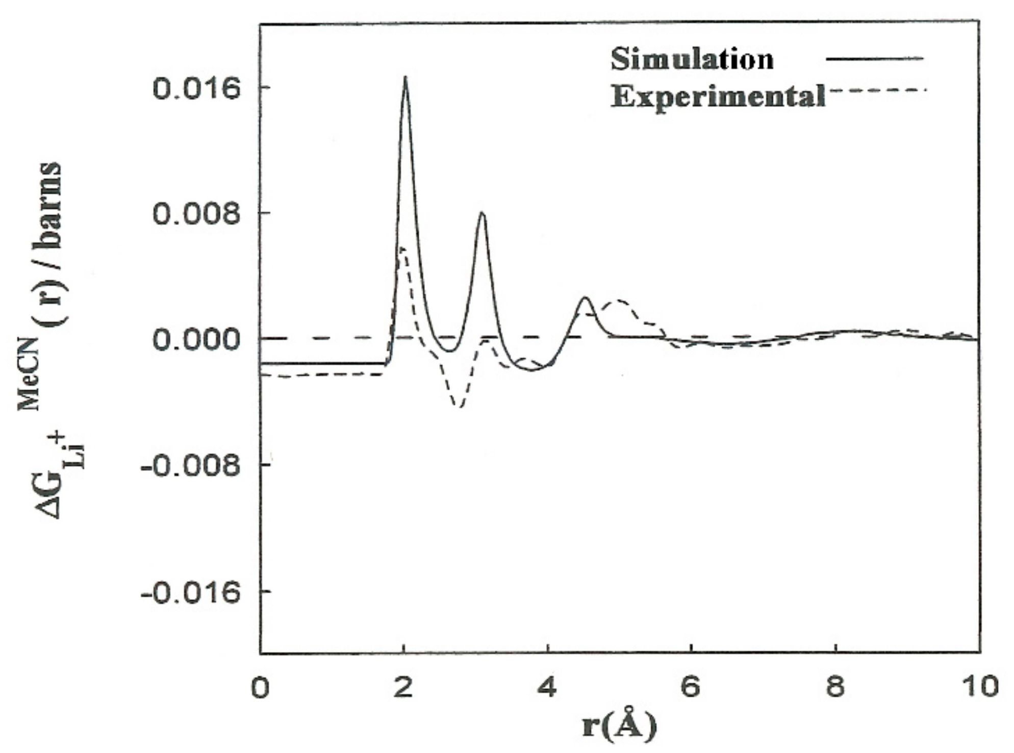The experimental solubility of LiBr in acetonitrile is 0.58 M. We calculated the $\mathsf{\Delta }{G}_{{\mathrm{Li}}^{+}}^{\mathrm{MeCN}}$ corresponding to this concentration from the $g_{I\mathrm{MeCN}}\left(r\right)$ for Li⁺ as follows:

$$\begin{gathered} \mathsf{\Delta }{G}_{{\mathrm{Li}}^{+}}^{\mathrm{MeCN}}\left(r\right) = A\left[g_{\mathrm{LiBr}}\left(r\right) - 1\right] + B\left[g_{\mathrm{LiLi}}\left(r\right) - 1\right] + C\left[g_{\mathrm{LiH}}\left(r\right) - 1\right] + \cdots \\ D\left[g_{{\mathrm{LiC}}_1}\left(r\right) - 1\right] + E\left[g_{\mathrm{LiN}}\left(r\right) - 1\right] + F\left[g_{{\mathrm{LiC}}_2}\left(r\right) - 1\right] \end{gathered}$$

(4)

where the constants A–F depend on the concentration and scattering lengths. The contribution of the first two terms of (4) pertains to distances beyond the first hydration shell, $A=B~0$. The shape of the $\mathsf{\Delta }{G}_{{\mathrm{Li}}^{+}}^{\mathrm{MeCN}}$ function resulting from the simulations is in agreement with the experimental results (Figure 3). We obtained the contribution to $\mathsf{\Delta }{G}_{{\mathrm{Li}}^{+}}^{\mathrm{MeCN}}$ for the last three terms of (4). The results are consistent with the interpretation regarding the principal $\mathsf{\Delta }{G}_{{\mathrm{Li}}^{+}}^{\mathrm{MeCN}}$ peaks. The discrepancies in the height of the $\mathsf{\Delta }{G}_{{\mathrm{Li}}^{+}}^{\mathrm{MeCN}}$ peaks can be attributed to the deficiency in the interaction potentials used, as well as to experimental inaccuracies and the hydrogen atoms of the methyl group not being taken into account. Nevertheless, nearly all of the computer simulation studies described for acetonitrile and acetonitrile solutions are based on the hypothesis of rigid molecular models that do not explicitly consider the hydrogen atoms of the methyl group. With this assumption, the computing time is substantially decreased, and longer simulations of larger systems can be carried out.

Table 4 summarizes the positions of the first peaks of $g_{I\mathrm{MeCN}}\left(r\right)$, and the coordination numbers obtained from our simulations and neutron diffraction experiments. The most probable distances, Li⁺-N and Li⁺-C, are well-reproduced. For Li⁺ in acetonitrile, we obtain a coordination number slightly higher than the experimental one (5.5 instead of 3). This failure of simulations can be attributed to the deficiency in the interaction potentials used and the hydrogen atoms of the methyl group not being considered explicit.

3.2. Mean Force Potentials

The force (∆F(t;r)) applied by N solvent molecules along the intermolecular axis of two A and B ions is indicated by:

$$\mathsf{\Delta }F\left(t;r\right) = \mu \left(\frac{F_{AS}\left(t;r\right)}{m_A}-\frac{F_{BS}\left(t;r\right)}{m_B}\right)·\widehat{r},$$

(5)

the resultant forces F_AS(t; r) and F_BS(t; r) acting on the solute caused by the molecular liquid, m_A and m_B are the masses of the solute, $\widehat{r}$ is the unit vector alongside the AB path and $\mu = m_A{m}_B/\left(m_A+m_B\right)$ is the reduced mass. This expression is calculated at every single time interval and averaged throughout the entire simulation. Where F_d(r) is the direct solute force, and the resultant MF between ions is:

$$F\left(r\right) = F_d\left(r\right) + \mathsf{\Delta }F\left(r\right),$$

(6)

where $\mathsf{\Delta }F\left(r\right) \equiv \langle \mathsf{\Delta }F\left(t;r\right)\rangle$. W(r) was calculated by integrating the mean force:

$$W\left(r\right) = W\left(r_0\right) - {{\displaystyle \int }}_{r_0}^r{F}_d\left(r\right)dr.$$

(7)

W(r₀) was calculated so the PMF values matched the macroscopic Coulomb potential at large distances ($r_0=9.0 \mathrm{\AA })$ and used the experimental acetonitrile relative permittivity (${\epsilon }_r^{\mathrm{MeCN}}=36$). Table 2 summarizes the range of interionic separation for each pair and the total number of simulations performed.

The statistical errors for W(r) and ΔF were analyzed as stated by the method outlined in the ref. [24].

Table 5. Error estimates: value to the ion–ion PMF ($k_{B}T/\mathrm{\AA }$).

Ion Pair	r/Å	${\mathit{S}}_{\mathbf{\Delta }\mathit{F}\left(\mathit{r}\right)}/\mathbf{ps}$	${\mathit{\tau }}_{\mathit{R}\mathit{U}\mathit{N}}=50 \mathbf{ps}$		${\mathit{\tau }}_{\mathit{R}\mathit{U}\mathit{N}}=75 \mathbf{ps}$		${\mathit{\tau }}_{\mathit{R}\mathit{U}\mathit{N}}=100 \mathbf{ps}$
			${\mathit{\sigma }}_{\mathbf{\Delta }\mathit{F}\left(\mathit{r}\right)}$	${\mathit{ϵ}}_{\mathbf{\Delta }\mathit{F}\left(\mathit{r}\right)}$	${\mathit{\sigma }}_{\mathbf{\Delta }\mathit{F}\left(\mathit{r}\right)}$	${\mathit{ϵ}}_{\mathbf{\Delta }\mathit{F}\left(\mathit{r}\right)}$	${\mathit{\sigma }}_{\mathbf{\Delta }\mathit{F}\left(\mathit{r}\right)}$	${\mathit{ϵ}}_{\mathbf{\Delta }\mathit{F}\left(\mathit{r}\right)}$
	2.2	0.30	9.51	0.74	9.05	0.57	8.87	0.48
Li+-Br−	4.4	0.05	14.16	0.45	14.23	0.37	14.90	0.33
	8.0	0.15	11.54	0.63	11.97	0.54	12.09	0.47
Li+-Li+	5.6	0.12	11.11	0.54	11.04	0.54	10.75	0.37
Br−-Br−	7.0	0.45	4.48	0.43	4.51	0.35	4.68	0.32

shows the statistical inefficiency ($s_{\mathsf{\Delta }F\left(r\right)}$), standard deviation (${\sigma }_{\mathsf{\Delta }F\left(r\right)}$) and estimated statistical errors (${ϵ}_{\mathsf{\Delta }F\left(r\right)}$) values according to several interionic distances and simulation lengths. Simulations beyond 50 ps provided no further benefit. The estimated errors for the mean force potentials for the various ion pairs range between $0.4 k_{B}T$ and $0.7 k_{B}T$.

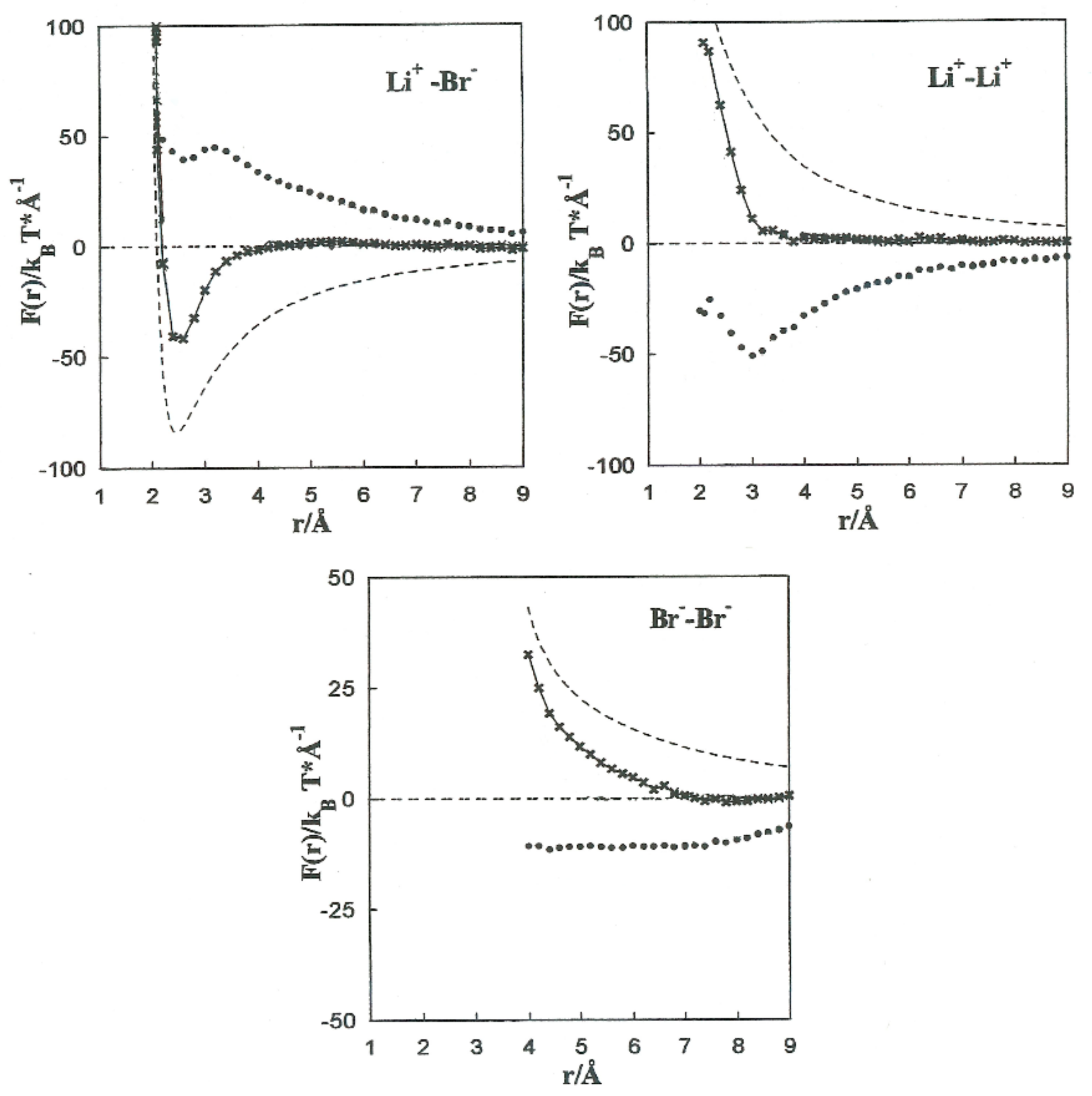
The MF acting on every single ion is shown in Figure 4, jointly with the direct (F_d) and solvent (∆F(r)) contributions to the Li⁺-Br⁻, Li⁺-Li⁺, and Br⁻-Br⁻ pairs. The contributions of the solvent (∆F(r)) are opposite to the direct ion–ion force in all the systems.

This is constant with the trend of polar liquids to produce stable complexes in the case of like-ion pairs, and to separate ions with opposite signs [2,3,4,5]. Equilibrium between the direct and solvent contributions results in a repulsive force acting on the Li⁺-Li⁺ pair at all distances. For the Li⁺-Br⁻ pair, the resultant force is repulsive at extremely small distances and attractive at middle separation. The total force on the Br⁻-Br⁻ pair has similar tendencies, but the attractive component is considerably less significant.

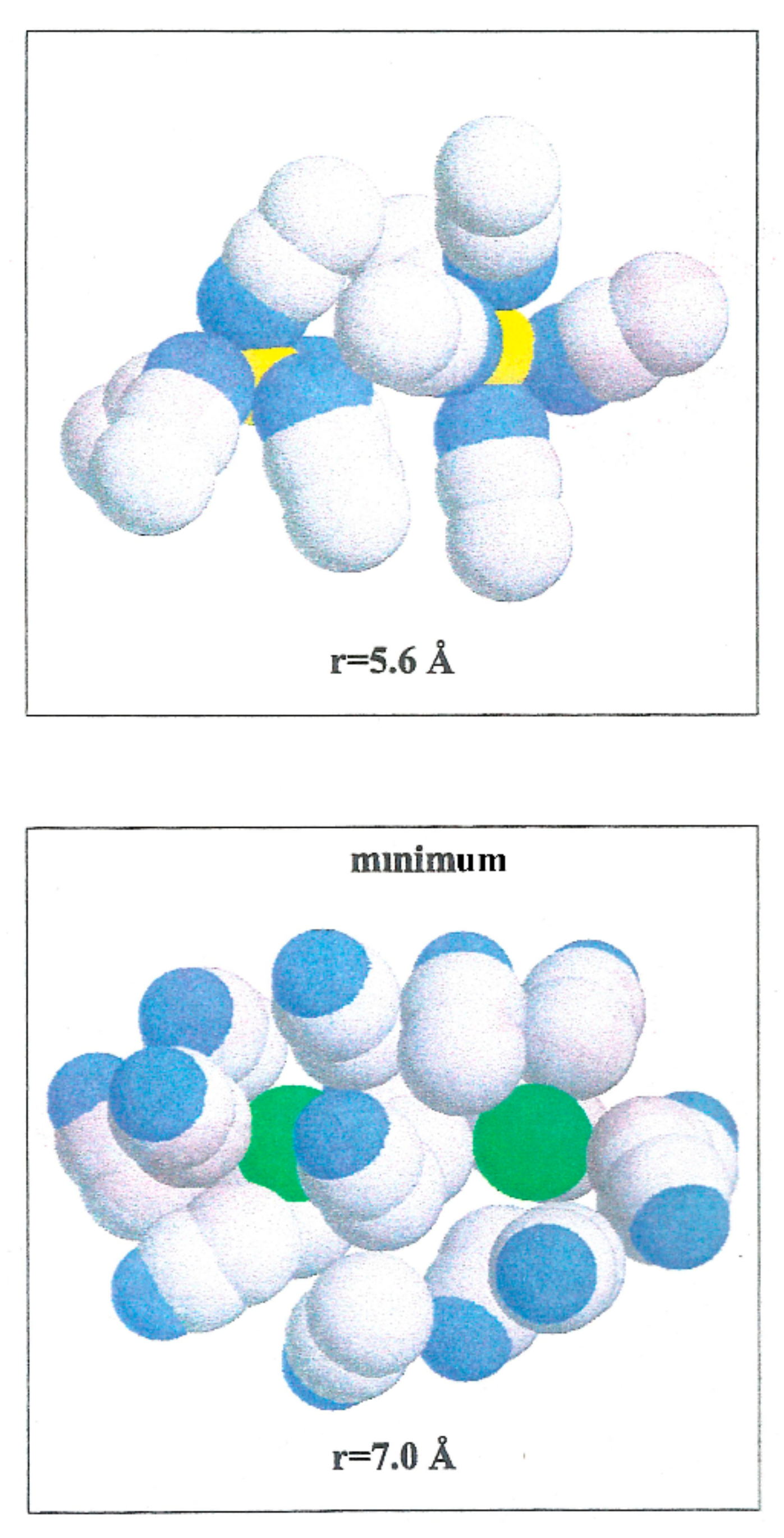
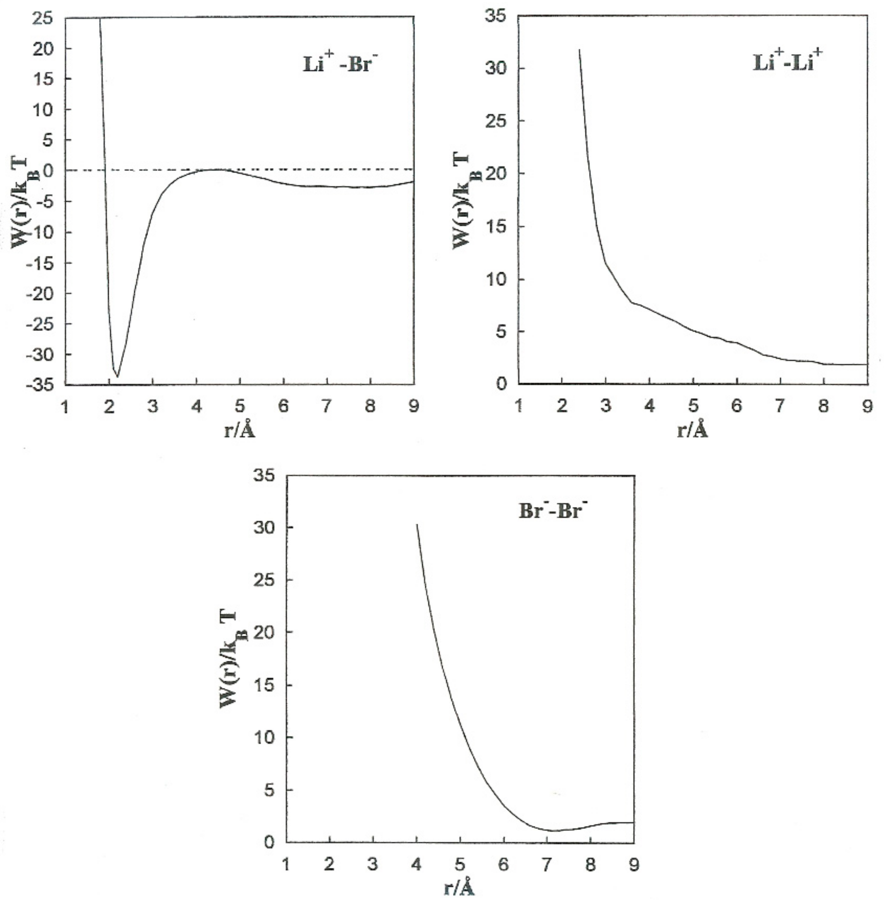
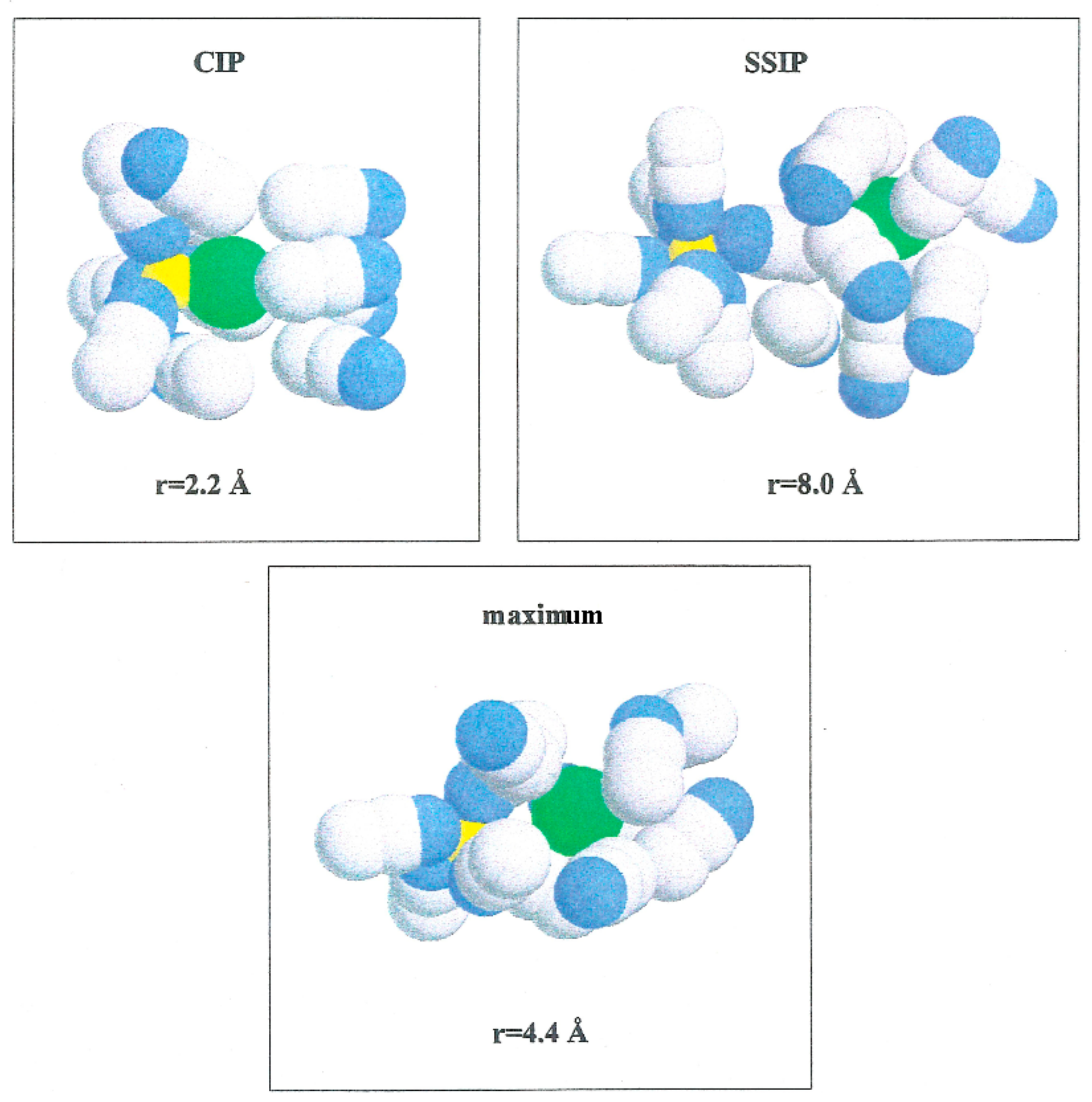
Figure 5 shows the PMF values for the various ion pairs. Oscillations in the potential corresponding to Li⁺-Br⁻ occur in association with the structure of the solvent in the vicinity of the ions. W(r) shows a noticeable minimum at 2.2 Å and lower one at 8.0 Å. The contact ion pair (CIP) region corresponding to the first minimum, and for the solvent separated ion pair (SSIP) region the second one. W(r) shows a maximum at r = 4.4 Å. In the CIP region, the ion pairs are enclosed by acetonitrile particles, with the corresponding nitrogen atoms geared to the Li⁺ and their methyl groups in the direction of Br⁻, as illustrated in Figure 6. The SSIP region values are attributed to attractive forces produced by solvent molecules between ion pairs.

The stability of the CIP and SSIP regions is indicated by the association constants [25]. For the CIP and SSIP state we have the following expressions

$$K_{CIP}=4\mathsf{\pi } N_A {{\displaystyle \int }}_0^{r_b}{e}^{-\frac{W\left(r\right)}{K_{B}T}} {r^{\prime }}^{2}d{r}^{\prime }$$

(8)

$$K_{SSIP}=4\mathsf{\pi } N_A {{\displaystyle \int }}_{r_b}^{r_m}{e}^{-\frac{W\left(r\right)}{K_{B}T}} {r^{\prime }}^{2}d{r}^{\prime },$$

(9)

where $N_A$ is the Avogadro’s number and $r_b$ is a cut-off parameter that we have chosen as the position of the first potential of mean force W(r) maximum, and $r_m$ is some value of r for which it is considered that the diffusive motion is a good approximation. Moreover, the equilibrium constant is giving by

$$K_{eq}=\frac{K_{SSIP}}{K_{CIP}},$$

(10)

we calculate the association constants $K_{CIP}$ and $K_{SSIP}$ and the equilibrium constant, as shown in

Table 6. Li⁺-Br⁻ association-dissociation barrier heights in $k_{B}T$ and association constants in 1/mol (ion–ion distances are in Å).

Magnitude	Value
$r_{CIP}$	2.2
$r_{max}$	4.4
$r_{SSIP}$	8.0
Dissociation barrier	33.7
Association barrier	2.9
$K_{CIP}$	$3.1\times {10}^{12}$
$K_{SSIP}$	22.0
$K_{eq}$	$7.1\times {10}^{-12}$

. We found that $K_{CIP}\gg K_{SSIP}$. The value obtained from the equilibrium constant ($K_{eq}=7.1\times {10}^{-12}$) indicates much less stable configurations in the SSIP region compared to the CIP region.

W(r) for Li⁺-Li⁺ is repulsive and decreases monotonically to zero. Even though the acetonitrile molecules located near the ion pairs have their nitrogen atoms toward Li⁺, as shown in Figure 7, the electrostatic interaction N-Li⁺ is less important than F_d.

The Br⁻-Br⁻ pair conformation is steadied at a separation corresponding to the minimum (r = 7.0 Å) of W(r) by the acetonitrile molecules enveloping it. Their methyl atoms are oriented toward the Br⁻ ions due to an attractive interaction. The structure is stabilized by the methyl atoms of the liquid molecule in the central area.

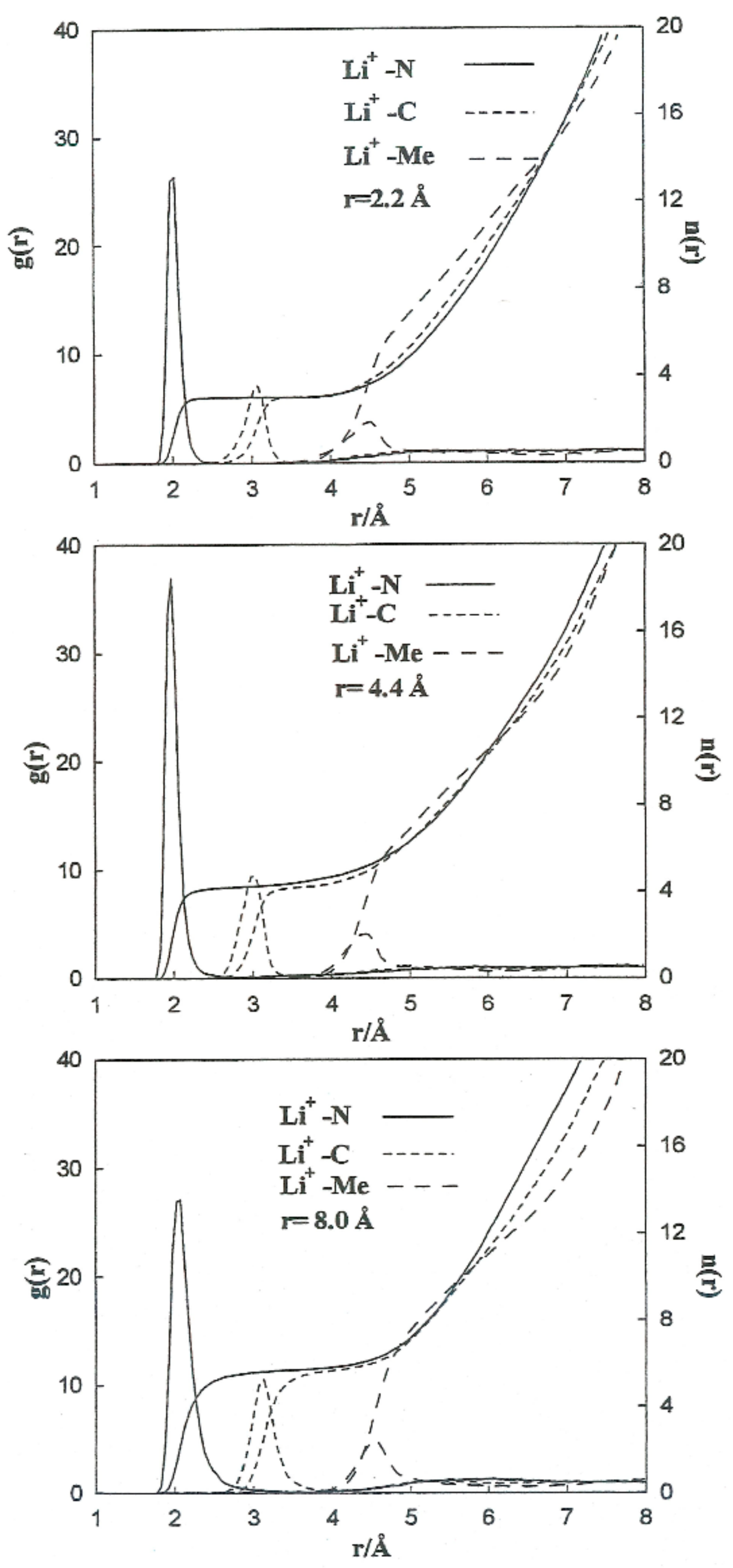
To carry out a more quantitative analysis of the distribution of the liquid molecules around the ionic particles, we determined the radial ion–solvent distribution functions (left axis) and their corresponding coordination numbers (right axis) for different interionic separations. Figure 8 and Figure 9 show the radial distribution functions, Ion-Me, Ion-C and Ion-N, obtained in the situation of the Li⁺-Br⁻ ion pair for the interionic separations corresponding to r_CIP, r_SIP and the maximum value of W(r).

Table 7. Maximum ($R_{ion-atom}$) and minimum ($r_{ion-atom}$) radial distribution functions for the various cases.

Ion-Pair	r/Å	${\mathit{R}}_{\mathit{i}\mathit{o}\mathit{n}-\mathbf{N}}$		$\mathit{g}({\mathit{R}}_{\mathit{i}\mathit{o}\mathit{n}-\mathbf{N}})$		${\mathit{R}}_{\mathit{i}\mathit{o}\mathit{n}-\mathbf{C}}$		$\mathit{g}({\mathit{R}}_{\mathit{i}\mathit{o}\mathit{n}-\mathbf{C}})$		${\mathit{R}}_{\mathit{i}\mathit{o}\mathit{n}-\mathbf{Me}}$		$\mathit{g}({\mathit{R}}_{\mathit{i}\mathit{o}\mathit{n}-\mathbf{Me}})$
		Li+	Br−	Li+	Br−	Li+	Br−	Li+	Br−	Li+	Br−	Li+	Br−
	2.2	2.025	3.575	26.3	4.3	3.075	4.575	7.1	2.8	4.525	3.925	3.7	3.3
Li+-Br−	4.4	1.975	4.325	36.9	1.7	3.025	3.975	9.4	2.2	4.575	3.875	3.4	4.6
	8.0	2.075	6.075	27.1.	1.7	3.125	4.925	10.4	2.2	4.525	3.875	4.9	5.3
Li+-Li+	5.6	1.975		27.8		3.075		10.0		4.525		4.6
Br−-Br−	7.0		5.675		1.5		4.775		2.2		3.875		5.3
Free ions		2.025	5.775	27.8	1.5	3.075	4.775	10.1	2.2	4.525	3.875	4.7	5.3
Ion-Pair	r/Å	$r_{ion-N}$		$g(r_{ion-N})$		$r_{ion-C}$		$g(r_{ion-C})$		$r_{ion-Me}$		$g(r_{ion-Me})$
		Li+	Br−	Li+	Br−	Li+	Br−	Li+	Br−	Li+	Br−	Li+	Br−
	2.2	2.825	4.075	0.0	0.2	3.575	6.225	0.0	0.6	6.475	5.225	0.6	0.7
Li+-Br−	4.4	3.075	4.825	0.1.	0.8	3.625	5.975	0.2	0.5	6.275	5.675	0.6	0.3
	8.0	3.675	7.875	0.1	0.8	3.975	6.125	0.2	0.6	6.275	5.925	0.5	0.4
Li+-Li+	5.6	3.375		0.1		3.875		0.4		6.125		0.6
Br−-Br−	7.0		8.025		0.7		6.025		0.5		5.675		0.4
Free ions		3.575	8.075	0.1	0.7	4.075	5.975	0.2	0.5	6.325	5.925	0.5	0.4

summarizes the positions of the maximum and minimum radial distribution functions for the various cases analyzed. The corresponding coordination numbers are given in

Table 8. Ion–solvent coordination numbers for each ion pair and interionic separation.

Ion Pair	r/Å	$\mathit{c}{\mathit{n}}_{\mathit{N}}$		$\mathit{c}{\mathit{n}}_{\mathit{C}}$		$\mathit{c}{\mathit{n}}_{\mathit{M}\mathit{e}}$
		Li+	Br	Li+	Br−	Li+	Br−
	2.2	3.0	3.0	3.0	11.5	12.9	7.5
Li+-Br−	4.4	4.2	3.4	4.2	9.7	11.4	9.5
	8.0	5.7	22.4	5.6	10.7	11.9	10.8
Li+-Li+	5.6	5.2		5.2		10.7
Br−-Br−	7.0		21.2		10.1		10.4
Free ions		5.5	23.3	5.5	9.8	11.9	10.7

. A coordination number ($c{n}_N$) of 23 for a free bromide ion in acetonitrile is large. This value may be attributed to the deficiency in the interaction potentials used. Nevertheless, other studies indicate that the solvation shell of the Br-anion can have a maximum number of molecules of acetonitrile bigger than 10 [9]. It should also be pointed out that in aqueous solutions coordination numbers increase when the concentration decrease [26].

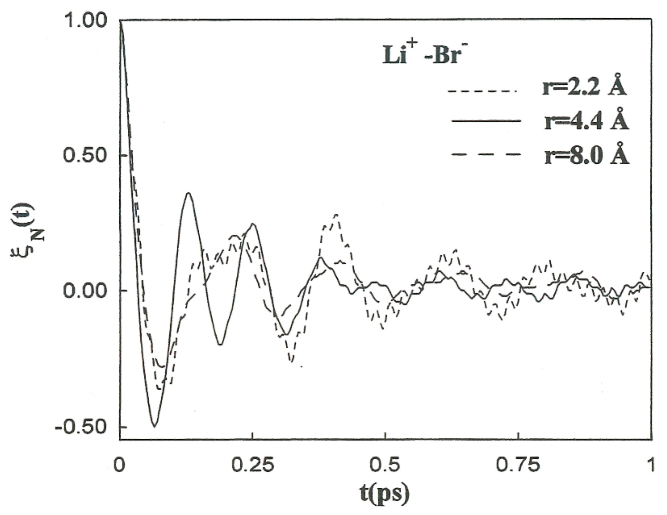
3.3. Li⁺-Br⁻ Interconversion and Friction Kernels

The friction kernels $\xi \left(t\right)$ depend on the ionic species and interionic distances [27].

We determined the transmission coefficient ($k$) of the barrier at 4.4 Å according to the Grote–Hynes theory of chemical reactions in a solution. In this model, the reaction coordinate develops by a global Langevin equation. The transmission coefficient (subscript GH or Kr stand for Grote–Hynes or Kramers) can be obtained as:

$$k_{GH}=\frac{{\lambda }_r}{{\omega }_b},$$

(11)

where ${\omega }_b$ is the barrier frequency, obtained by extrapolating an inverted parabola with an apex equivalent to the maximum PMF value. ${\lambda }_r$ (reactive frequency) is the result of the next expression:

$${\lambda }_r=\frac{{\omega }_b}{\left[{\lambda }_r+{{\displaystyle \int }}_0^{\infty }\xi \left(t\right)e^{-{\lambda }_{r}t}dt\right]}.$$

(12)

It is follows that ${\lambda }_r$ is the characteristic frequency for the unstable motion at the transition state. For the coefficients involved in the previous theory regarding the Li⁺-Br⁻, Li⁺-Li⁺, and Br⁻-Br⁻ systems, the initial values of the friction kernels ($\xi \left(0\right))$ are summarized in

Table 9. Initial values of the friction kernels for all ion pairs and interionic separations.

Ion Pair	r/Å	$\mathit{\xi }\left(\mathbf{0}\right) \times {\mathbf{10}}^{\mathbf{-}\mathbf{3}}$ (ps−2)
	2.2	2.98
Li+-Br−	4.4	8.55
	8.0	5.69
Li+-Li+	5.6	8.18
Br−-Br−	7.0	0.14

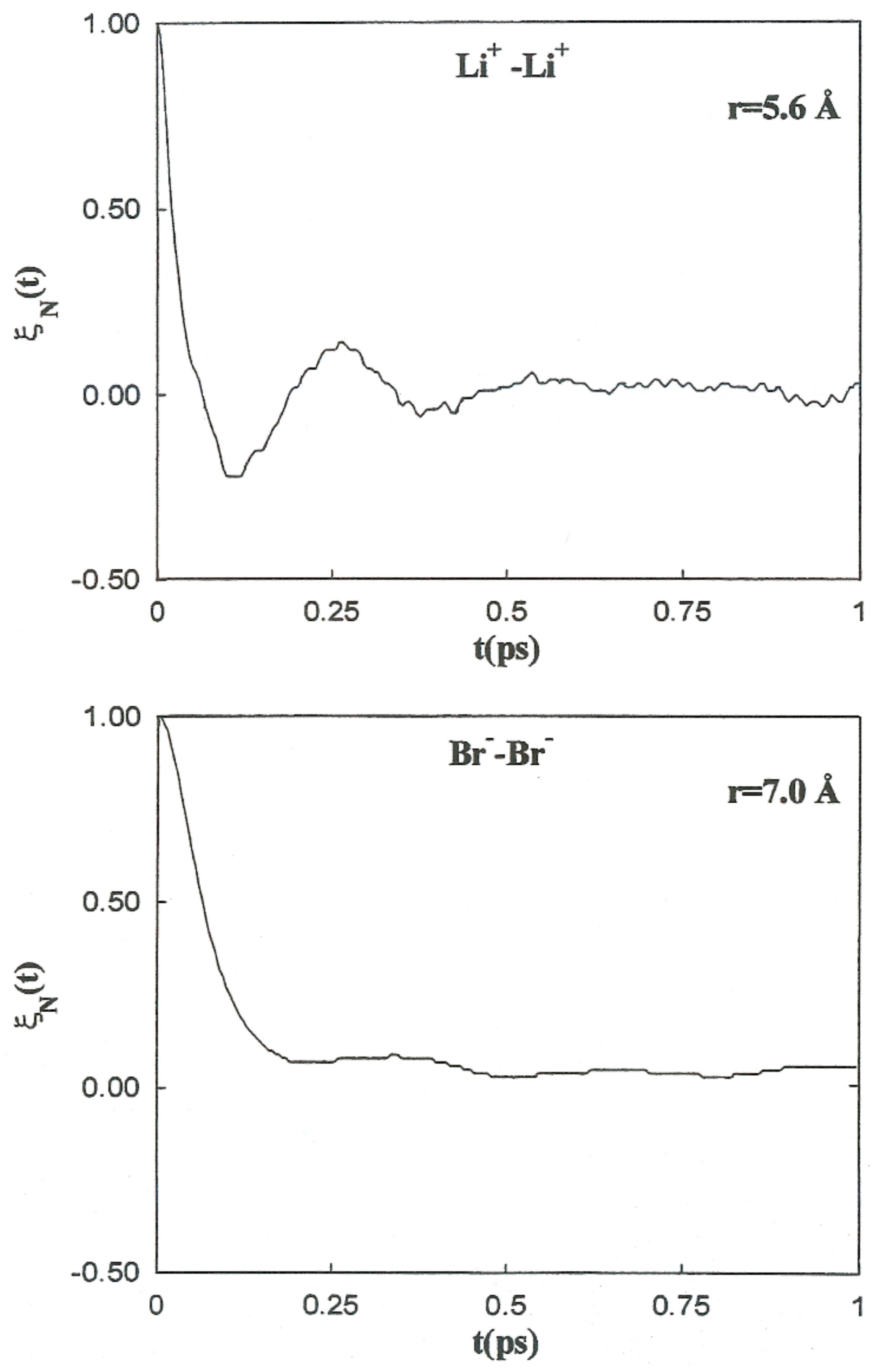
. The initial time values of the $\xi \left(t\right)$ kernels are not only dependent on the ionic species but also show noticeable changes with the interionic separation. This interionic separation dependence of $\xi \left(0\right)$ is strongly related to the magnitude of the changes in the solvent structure around the ion pairs as a function of these separations. The normalized friction kernels (${\xi }_N\left(t\right) = \xi \left(t\right)/\xi \left(0\right)$) related through all cases are displayed in Figure 10 and Figure 11. There are features common to the functions of both systems, all of which show a rapid and very similar initial decay before 0.2 ps. A lengthy decay follows, characterized for each individual system.

The coefficients involved in the Li⁺-Br⁻ system are summarized in the

Table 10. Li⁺-Br⁻ association-dissociation process parameters and reaction constants.

Magnitude	Value
${\omega }_b\left({\mathrm{ps}}^{-1}\right)$	8.2
$\xi \left({\mathrm{ps}}^{-1}\right)$	165
$k_{kr}$	0.050
$k_{GH}$	0.056
${\lambda }_r^{-1}\left(\mathrm{ps}\right)$	2.17
${}_c\left(\mathrm{ps}\right)$	0.019
${\omega }_{NA}^2\left({\mathrm{ps}}^{-2}\right)$	$-8.48\times {10}^{-3}$
$k_f\left({\mathrm{ps}}^{-1}\right)$	$4.8\times {10}^{-15}$
$k_b\left({\mathrm{ps}}^{-1}\right)$	$1.2\times {10}^{-3}$
${\left(k_f+k_b\right)}^{-1}\left(\mathrm{ps}\right)$	835

.

${\lambda }_r^{-1}$, gives us a temporal measure of the transition state in the presence of the solvent. We determined that, for acetonitrile, ${\lambda }_r^{-1}=2.17 \mathrm{ps}$.

The correlation time of the friction of the solvent acting on the ion pair (${\tau }_c)$ is defined by the value of the integral of the normalized kernel function:

$${\tau }_c={{\displaystyle \int }}_0^{\infty }{\xi }_N\left(t\right)dt.$$

(13)

In the case of acetonitrile, the correlation time is shorter than the reaction time.

A polarization caging regime is verified because a negative amount for the nonadiabatic barrier frequency (${\omega }_{NA}^2={\omega }_b^2-\xi \left(0\right))$ was found [28]. In this regime, the solvent immediately catches the solute in a well or “polarization cage” of solvent molecules. Hence, the motion of solvent molecules is extremely crucial. A limiting case of the polarization caging regime is when ${\tau }_c\ll {\lambda }_r^{-1}$ and designated as adiabatic. In such circumstances, the predictions of the Grote–Hynes theory are reduced to Kramers doublets. Our results confirm that for the Li⁺-Br⁻ ion pair, $k_{GH}\simeq k_{kr}$.

Lastly, we computed the full rate constants for the dissociation ($k_f$) and association ($k_b$) processes, given by [27,29]:

$$k_f=\frac{k_{GH}}{\sqrt{2\pi \beta {\mu }_I}}\cdot \frac{{\left(r^{\ne }\right)}^2{e}^{-\beta W\left(r^{\ne }\right)}}{{{\displaystyle \int }}_0^{r^{\ne }}{r}^2{e}^{-\beta W\left(r\right)}dr}$$

(14)

$$k_b=\frac{k_{GH}}{\sqrt{2\pi \beta {\mu }_I}}\cdot \frac{{\left(r^{\ne }\right)}^2{e}^{-\beta W\left(r^{\ne }\right)}}{{{\displaystyle \int }}_{r^{\ne }}^{r^m}{r}^2{e}^{-\beta W\left(r\right)}dr},$$

(15)

whereby ${\mu }_I$ is the reduced mass of the ion pair, $k_{GH}$ is the transmission coefficient, $r^{\ne }$ is the interionic separation at the transition state (i.e., the top barrier), $\beta =1/k_{B}T$ and $r_m$ is an arbitrary interionic distance beyond the outer boundary of the SSIP region, where there is no further interactivity. The results are summarized in Table 10. We have obtained a $k_f$ rate constant that is roughly smaller than $k_b$. This is due to the greater stability of the CIP complex for the present model system since a value of $7.1\times {10}^{-12}$ was obtained for $K_{eq}$. Our overall constant rate ${\left(k_f+k_b\right)}^{-1}$ corresponds to a relaxation time of approximately 835 ps. Values for ${\tau }_c=0.019 \mathrm{ps}\ll {\lambda }_r^{-1}=2.17 \mathrm{ps}$ were found. In such circumstances, the predictions of the Grote–Hynes theory are reduced to Kramers doublets. From the transmission coefficient values ($k_{GH}=0.050; k_{kr}=0.056$) results confirm the case called regime adiabatic and for the Li⁺-Br⁻ ion pair, $k_{GH}\simeq k_{kr}$. A polarization caging regime is verified because a negative amount for the nonadiabatic barrier frequency (${\omega }_{NA}^2=-8.48\times {10}^{-3} {\mathrm{ps}}^{-2})$ was found.

4. Conclusions

The results reported in this paper on structural properties are in agreement with the experimental data; for instance, we carried out two unconstrained simulations of Li⁺ and Br⁻, with 215 solvent molecules. The information obtained from these ion–solvent structure simulations is compared to the neutron diffraction data (Table 3). We also obtain a coordination number for Li⁺ in acetonitrile, slightly higher than the experimental one (5.5 instead of 3—Table 4). This failure of simulations can be attributed to the deficiency in the interaction potentials used and the hydrogen atoms of the methyl group not being considered. We obtained PMF values for Li⁺-Br⁻, Li⁺-Li⁺, and Br⁻-Br⁻. For the Li⁺-Br⁻ ion pair, the diluter allows sets two stable interionic separations, a CIP and a SSIP; where the CIP is more stable. The Li⁺-Li⁺ system is repulsive. The Br⁻-Br⁻ pair composition is equilibrated at a distance corresponding to the lowest value (r = 7.0 Å) of W(r) by the adjacent acetonitrile molecules. The friction kernels and interconversion process of the Li⁺-Br⁻ ion pair were evaluated. The passage of the barrier happens in the polarization caging regime. The correlation time of the solvent ${\tau }_c$ is much shorter than the reaction time ${\lambda }_r^{-1}$ and the Kramers regime of the Grote–Hynes theory was found for the system.