Abstract
In this review article, we survey some of our results pertaining to the search for the electric dipole moment of the electron (eEDM), using heavy polar molecules. In particular, we focus on the relativistic coupled cluster method (RCCM) and its applications to eEDM searches in YbF, HgX (X = F, Cl, Br, and I), BaF, HgA (A = Li, Na, and K), and YbOH. Our results are presented in a systematic manner, by first introducing the eEDM and its measurement using molecules, the importance of relativistic many-body theory, and finally our results, followed by future prospects.
1. Introduction
The electric dipole moment of the electron (eEDM), which is a parity (P) and time (T) reversal violating property [1,2], is of immense interest in probing fundamental physics, especially beyond the Standard Model (BSM) theories. The Standard Model (SM) predicts a small value for eEDM ( e-cm), as compared to many BSM theories, which predict the eEDM to be several orders of magnitude larger [3] (see Figure 1). Therefore, by comparing experimental upper bounds on the eEDM (the eEDM has not been detected yet, in over six decades of ever-improving experiments) with those predicted by several BSM theories, one can stringently constrain the latter. The general interest in this field is compounded by the fact that high precision eEDM search experiments are non-accelerator approaches that complement accelerator searches, but can explore much higher energy scales, as high as PeV [4]. The eEDM can also throw light on the baryon asymmetry in the Universe [5], which attempts to address why our Universe is matter-dominated, while one may expect an early Universe to be created with equal amounts of matter and anti-matter. This connection is associated with the fact that both the not-yet-measured eEDM and the well known value of baryon asymmetry coefficient are CP violating (T violation implies CP violation, due to the CPT theorem [6]). Further details can be found in Ref. [7].
The current best limits for the eEDM are from heavy polar molecules (all at 90 percent confidence intervals): ThO ( e-cm; e-cm; the subscripts ‘stat’ and ‘sys’ refer to the uncertainties due to statistics and systematics, respectively) [8], followed by HfF ( e-cm; e-cm) [9], and YbF ( e-cm; e-cm) [10,11]. Two experiments that employ BaF to probe the eEDM are currently underway [12,13,14]. An eEDM experiment that commenced recently (called the polyEDM experiment) using YbOH is expected to improve the sensitivity further in the future [15].

Figure 1.
(a) One-loop Standard Model (SM) contribution to the electric dipole moment of the electron (eEDM). The phases in the two vertices cancel out, leaving behind no charge–parity (CP) violating contributions, resulting in zero eEDM at the one-loop level. (b) It turns out that there are no contributions at the two- and three-loop levels either; a sample three-loop diagram has been given above, and although an individual three-loop diagram itself may not vanish, the non-zero diagrams eventually cancel out [16], (c) The first non-zero contribution to the SM eEDM occurs at the four-loop level [17], and (d) supersymmetry (SUSY) contribution to the eEDM. The phases at the two vertices are different, and therefore, one can obtain a non-zero contribution to the eEDM at the one-loop level itself. This is also why the eEDMs in most beyond the SM (BSM) are much larger than their SM counterpart [3].

This article is structured as follows: since the introduction section covers the eEDM, we shall discuss about eEDM searches in molecules in the next section, followed by a brief discussion on relativistic many-body theory with focus on the relativistic coupled cluster method (RCCM), after which we shall present some of our results for YbF, HgX (X = F, Cl, Br, and I), BaF, HgA (A = Li, Na, and K), and YbOH. We shall use atomic units in this article, unless explicitly stated otherwise.
2. eEDM Searches in Molecules
2.1. The Effective Electric Field
A high precision experiment that directly uses an electron beam, for example, would be extremely difficult, as the particle would accelerate away in the presence of an electric field. Instead, one uses atoms or molecules as proxies, and measures the shift in their energy level due to the eEDM. We shall only consider heavy polar molecules in this article, as molecules are preferred over atoms due to their higher experimental sensitivity. The shift in the energy of a molecule () that is prepared in some state, due to the eEDM (), is given by
where is called the effective electric field, since it has the same dimensions as an electric field. The expression for can be obtained by starting with the eEDM Hamiltonian [18]
The above expression is basically the well-known - expression for the interaction potential for a dipole, d, in an electric field, E, except that the dipole here is the eEDM that lies along the spin axis [19] (; is the Pauli matrix), while the field in this case is an internal electric field, . The internal electric field, , experienced by an electron, is due to the nuclei and all the other electrons in the molecule. The Dirac matrix denotes that we work in a relativistic regime. A relativistic treatment is necessary, since otherwise, the effective electric field is zero, due to the Schiff’s theorem [20]. The summation is over the number of electrons, . Because the eEDM is an extremely small quantity, the shift in energy due to it, to first order in perturbation, can be expressed as
In the first equation given above, is the unperturbed wave function of a molecule. We note that although the eEDM operator is parity-odd, the resulting expression for with respect to the unperturbed wave function is non-zero, unlike an atomic case. This is because one expands the molecular orbitals (MOs) contained in a molecular wave function as a linear combination of ‘atomic orbitals’ (AOs; strictly speaking, basis functions), often called the Linear Combination of Atomic Orbitals-Molecular Orbital (LCAO-MO) approach. This leads to mixing of opposite parity orbitals, and therefore a non-zero contribution. From Equations (1) and (3), one obtains
As seen earlier, the internal electric field, , experienced by the ith electron, includes contributions from each of the nuclei as well as from the other electrons. Since the latter leads to a term containing a two-body operator, directly calculating it is computationally very expensive. Hence, one employs an effective eEDM Hamiltonian, , whose expectation value is same as that of the original , when is the exact eigen function of the unperturbed Hamiltonian. Further details can be found in Refs. [21,22]. Hence, the effective electric field is given by
In the above expression, is the product of Dirac matrices, while is the momentum operator.
2.2. eEDM: A Combination of Experiment and Theory
As seen earlier in Equation (1), an eEDM experiment measures a shift in energy E, due to the eEDM, of a molecule prepared in a particular state. However, we need to revisit Equation (1) and slightly modify it, in order to accommodate for the dependence of the sensitivity to an external electric field that is applied to polarize the molecules. Therefore, one obtains
We see from the above expression that , which is called the polarizing factor, carries with it the information pertaining to the applied electric field (), the molecular permanent electric dipole moment (also known as the PDM, denoted by D), and the energy difference between rotational states of the molecule, . Often, for systems, one defines a polarizing field, (where B is the rotational constant of the molecule, and is related to ), which sets the scale for the required external electric field in order to polarize the molecules. It is desirable to be able to polarize a molecule with as low an external electric field as possible, or as low an as possible. Therefore, a molecule with a very low PDM can actually hamper the prospects of an otherwise good eEDM experiment, and hence, polar molecules are the preferred choices. The shift in energy is measured in experiment, the polarizing factor can either be calculated or found from experiment, while can only be calculated using a relativistic many-body theory. Therefore, an eEDM experiment is one of those branches in physics where experiment and theory go hand in hand. Also, it is worth noting at this point that the eEDM itself is a particle physics property that answers deep questions such as the matter-antimatter asymmetry in the universe (which is on a significantly different length scale), while the property can be measured by a combination of high-precision molecular experiments and relativistic many-body theory (involving quantum chemistry).
2.3. Choosing a Molecular Candidate
The statistical sensitivity of an eEDM experiment is given by
N refers to the number of molecules used per coherence time. T refers to the total interrogation time, while is the coherence time of the state of interest to an eEDM experiment. The importance of can be immediately understood from the above expression; it occurs outside the square root, and therefore plays a significant role in the sensitivity of an eEDM experiment.
The choice of a good eEDM candidate molecule usually relies upon the above mentioned factors (besides the effects of systematics and the prospects that a molecule offers for rejection of certain systematic effects). Not all of them can be satisfied in any one system; however, one looks for a suitable combination of these parameters to propose a new candidate which can potentially set a better bound on the eEDM. The effective electric field in a reasonably good molecular eEDM candidate is extremely large, and is usually ∼GV/cm (as compared to atoms, whose ‘’ for a ∼10 kV/cm field is ∼MV/cm). This is one of the major reasons why molecules are preferred over atoms.
3. Relativistic Many-Body Theory
We need to evaluate the expression given in Equation (5), in order to obtain . The molecular wave function in the expression has to be obtained from a relativistic many-body theory. We employ the relativistic coupled cluster method (RCCM) for our accurate calculations. Solving the RCCM equations rely upon the relativistic Hartree–Fock (HF) or Dirac–Fock (DF) reference state, and therefore, we shall briefly explain the DF equations, and then motivate RCCM by drawing parallels with the more intuitive many-body perturbation theory (MBPT).
3.1. The Dirac–Fock Method
The HF equations and its relativistic counterpart, the DF equations, can be obtained by applying the variational principle, which guarantees that the energy thus obtained would be an upper bound to the actual ground state energy (for example, Ref. [23]). The equations are
There are N such equations for an N-electron system, each corresponding to the ith spin-orbital, (the many-body wave function itself is built from these spin-orbitals, or single particle wave functions, as a Slater Determinant, ). The operator, contains in it the kinetic and the electron-nucleus interaction terms, and is the familiar electron-electron interaction term. The summation j is over the number of electrons in the system. The second and third terms are called the direct and the exchange terms respectively. Written in this form, the Hd or DF equations reveal the physical meaning of the direct term. By rearranging the direct term, one can readily see that it leads to a mean field interpretation, that is, each electron experiences an average potential due to the remaining () electrons. The exchange term has no classical counterpart. Also, in this form, it is transparent that the equation has to be solved in a self-consistent way, starting with an initial guess for the spin-orbitals.
In the DF method, one employs a relativistic Hamiltonian, that is, the Dirac–Coulomb Hamiltonian (DCB), , given by
The summation, i (and j), is over the electrons, while A is over the nuclei. and are the Dirac matrices, while is the momentum operator. is the atomic number of the Ath nucleus. is the position vector from the origin to the site of the ith electron, and is that from the origin to the site of the Ath nucleus. In practice, the third term would correspond to a finite nucleus, and we have given the point nucleus case above for simplicity. We work in the Born–Oppenheimer approximation, where the nuclei are ‘clamped’, and also in the no-pair approximation [24], where one projects out the negative energy solutions from the electronic Hamiltonian.
Also, the single particle wave function, for a relativistic case, is built from four-component spinors, given by
where v and w are referred to as the large and small components respectively, and in practice, are related to one another by the kinetic balance condition. The condition guarantees that the expression for kinetic energy is recovered in the non-relativistic limit, and also aids in avoiding variational collapse [25,26].
We shall now briefly discuss the matrix formulation of the DF equations, by first rewriting Equation (8) (we drop the co-ordinate labels for simplicity) as follows
Here, is a general spin-orbital. Let . Then,
Expanding as a linear combination of a suitable basis set, that is, , and projecting from the left with , one obtains.
The DF coefficients, , are what one solves for. is the overlap integral. It is now straightforward to recast the above equations in a matrix form as
After performing the similarity transform shown above, the resulting equation, that is, Equation (18), is solved iteratively to obtain the coefficients. Note that the choice of basis is one of the factors that determines the precision of a calculation. The other important factor that determines the precision is electron correlations, which we shall discuss next.
3.2. Electron Correlation
The HF method (and its relativistic counterpart, the DF method) is a mean field approach, which ignores the fact that every electron actually interacts with each of the remaining electrons. The physical effects beyond those embodied in the mean field approximation are subsumed under the umbrella of electron correlation.
If E is the energy that one obtains by solving the Schroedinger’s equation exactly, and if is the DF energy for the same system, then the correlation energy, , is
Some well known examples of many-body theories that take into account electron correlation effects are configuration interaction (CI), multi-configuration Hartree–Fock (MCHF), many-body perturbation theory (MBPT), coupled cluster Methods (CCM), and their relativistic extensions.
3.3. Many-Body Perturbation Theory: Non-Relativistic and Relativistic
To introduce MBPT, we define zeroth-order Hamiltonian () as a sum of Fock operators
For this Hamiltonian, the Hartree–Fock determinant () and its k-particle k-hole excitation determinants () become eigen functions of , and hence
In this picture, a hole refers to an occupied orbital, while a particle to an unoccupied/virtual one. Electron correlation effects are taken into account by accommodating for such virtual excitations to the HF wave function. Also, ; where the second term contains the orbital energies associated with a k particle-k hole excitation. For example , for one-particle one-hole and two particle-two hole cases, we obtain
respectively. In this notation, i, j, k, ⋯ are holes, and a, b, c, ⋯ are particles.
We now introduce a perturbation to the Hamiltonian, which is the difference between the actual and the HF potential. Then, the Schroedinger’s equation corresponding to the actual wave function of the system would be
where contains one order of , contains two orders of , etc.
This framework is common for both the relativistic (denoted by the subscript, ‘rel’) and non-relativistic cases (denoted by the subscript, ‘NR’), with the orbitals being different (four-component), and the one-body part of the Hamiltonian also differing as follows
with being a shorthand for for a point nucleus, or a suitable expression for a finite nucleus, depending on whether it is a Fermi or a Gaussian one.
4. Relativistic Coupled Cluster Method
The RCCM is a very accurate approach to treat electron correlation effects. To that end, the method has been referred to as the gold-standard of many-body theory of atoms and molecules. The RCCM wave function is given by
is called the cluster operator. For an N-electron system, . Here, , where all possible one-particle one-hole excitations are accounted for by the summation, is called the t-amplitude, which is like a weight factor for a one-particle one-hole excitation, and is a shorthand notation for , where a hole ‘i’ is annihilated and a particle ‘a’ is created. Similarly, , etc. One must also include all possible combinations of two independent one-particle one-hole excitations (given by ), a one-particle one-hole and a two particle-two hole occurring independently, but again all such possibilities (that is, ), and so on. By taking into account all such options and accounting for over-counting, we naturally obtain an exponential structure, that is, Equation (30) [27].
4.1. RCCM and MBPT
We shall now compare RCCM with MBPT. We begin by examining the full MBPT wave function, and then connecting it with RCCM.
Equations (32) and (33) involve rewriting the corrections to the wave function at a given order of perturbation, as a summation over single (that is, one-particle one-hole, and denoted by subscript S), double (D), ⋯ excitations. If we plug in Equations (32) and (33), and the rest of the corrections to the wave function to infinite orders, and rearrange, the resulting equation as
We see that this is actually the coupled cluster wave function. This correspondence is allowed, as the wave functions obtained from full MBPT and CCM without any truncation have to be the same. Equation (34) shows that for a given level of particle-hole excitation, CCM contains in it those excitations to all orders of perturbation in the residual Coulomb interaction. RCCM is also both size extensive and size consistent. Further details can be found in Ref. [28].
4.2. The Energy and Amplitude Equations
The RCCM equations that are to be solved, in order to obtain the t amplitudes, can be derived as follows
In Equation (38), we have projected Equation (37) with the DF wave function and in Equation (39), could be , , and so on. One can also write as , according to the linked cluster theorem. We shall briefly outline the derivation of the linked cluster theorem here. Given an operator , can be expressed as a sum of nested commutators, by using the Baker–Campbell–Hausdorff expansion. By using suitable arguments from the second quantization formalism, one can show that each of the terms in the sum are fully contracted, or in the diagrammatic approach, fully connected (denoted by the subscript, ‘c’), leading to the final expression [29]. Finally, we note that the expression for energy is naturally terminating, as this shall have important consequences later in this article.
4.3. The CCSD Approximation
One often works with the coupled cluster singles and doubles approximation (CCSD, or its relativistic counterpart, RCCSD), where . In such a case, the energy and amplitude equations are
After solving the amplitude equations and obtaining the wave function of the system, the next step would be to obtain the property of interest, for example, . This can be done in two ways, by either solving an expectation value problem, or by adopting an energy derivative approach. We shall discuss both these approaches below.
4.4. The Expectation Value Approach
The expectation value of an operator, , in RCCM is given by
The last equation was derived by Cizek [30,31]. The subscript ‘N’ means that the operator is normal ordered [32], while ‘C’ stands for fully connected, as seen earlier. This approach has the advantage of making the underlying physics more transparent, as one can break an expectation value expression down into its constituent terms, which in turn can be associated with several many-body effects, such as Bruckner pair correlation. However, the expectation value expression given above is an infinite, non-terminating series, and therefore requires that one manually truncate the expression, for obtaining a result. One such approximation is the linear expectation value approximation (LECC), which we have adopted. The expectation value in the CCSD approximation is then given by
As we shall see later, this turns out to be a good approximation for computing , for many systems with one unpaired electron.
4.5. The Energy Derivative Approach
The second approach relies on evaluating a property as an energy derivative. The derivative is taken with respect to a perturbation parameter, . The total Hamiltonian, (), is given by
Then,
Also,
From perturbation theory,
Within the RCCM framework, this approach takes advantage of the fact that the expression for coupled cluster energy naturally terminates. A first order property like or PDM could be evaluated as an energy derivative, either analytically (i.e., analytical derivative) or numerically (i.e., the finite field method). In our work, we have implemented the latter. We note that our discussions are based on computing first order properties like and PDM. The approach can be extended in a straightforward way to higher order properties, such as polarizabilities and hyperpolarizabilities.
We shall now explain some details of our implementation. We use an unrelaxed version of finite field coupled cluster method (FFCC), that is, we solve the unperturbed DF equations, and add the perturbation at the CCSD level. We shall derive an expression for CCSD correlation energy () with the perturbation lambda, as follows.
Using the fact that , and operating with on both sides on the left, we obtain
Using the linked cluster theorem, our correlation energy is
We note that the effects associated with orbital relaxation would be recovered at the perturbed CCSD level; for example, see Ref. [33]. The next step is to evaluate the energy derivative. Depending on the degree to which we wish to minimize the truncation error in a calculation, we can opt for a two-point central difference formula or beyond to evaluate the derivative. The two-point and the six-point formula are, respectively
The property of interest is obtained by adding its DF contribution to the above formula, that is,
The above equation can be obtained for a forward difference formula, for example, by starting with and E, and taking the difference. If the perturbation is , and is , then one obtains , or with an electric field as the perturbation, with being the dipole operator, one gets the PDM.
This approach offers the advantage of not having to truncate an infinite series in order to obtain a property. However, it is extremely time consuming, as one has to carefully choose the right value of , and a two-point central difference formula means that one has to evaluate the CCSD equations twice for one property.
4.6. Methodology
For all our results, we performed the DF calculations and obtained the property integrals using the UTChem package [34,35,36]. The same program was also used for atomic orbital to molecular orbital integral transformation. We then employed the Dirac08 program [37] to solve the CCSD equations and obtain the t amplitudes, and finally, we used our expectation value code for the LECC computations. For a finite field calculation, we introduce the perturbation at the CCSD level. Therefore, the one-electron integrals as well as the relevant property integrals with a chosen value of the perturbation parameter are fed to the Dirac08 program to obtain the energies. Further details on LECC approach can be found in Ref. [21], while Ref. [38] provides more information on the FFCC approach.
5. Results
5.1. First Application of RCCM to YbF
YbF currently holds the third best limit on the eEDM, and improvement in its current sensitivity is expected in the near future. We performed our first accurate molecular RCCM calculations on YbF, and using the LECC approach, obtained a value of −23.1 GV/cm for (see Table 1), with an estimated error of less than 10 percent [21]. A fairly large quadruple zeta (QZ) basis (primitive Gaussian basis sets) was used (Yb: (35s,30p,19d,13f,5g,3h,2i), F: (13s,10p,4d,3f)) [39,40,41]. We used a bond length of 2.0161 Angstroms [42]. Our result was an improvement over the previous ones, as they were based on the DF approximation [43], MBPT [44], effective core potential methods [45], and the CI method in the singles and doubles approximation [46]. The latest result on the molecule uses a complex generalized Hartree–Fock and a complex generalized Kohn-Sham scheme within the zeroth order regular approximation [47]. We had also systematically investigated the behaviour of as well as the PDM with change in the number of virtuals and frozen orbitals. Additionally, we also presented the individual correlation contributions, from Equation (46), at the QZ level of basis. In conclusion, our accurate result leads to an increase in the value of the upper bound on the eEDM to e-cm, as compared to the earlier result of e-cm. Further details can be found in Ref. [21].

Table 1.
Summary of the calculated linear expectation value approximation (LECC) results in YbF using a quadruple zeta (QZ) basis.
5.2. Mercury Halides
It was seen from Equation (7) that a large value of would substantially improve the statistical sensitivity of an eEDM experiment. We had identified that mercury halides, HgX, possess −100 GV/cm (see Table 2) [48], which is one and a half times larger than that of the current best candidate, ThO, and about five times that of YbF and HfF. We estimate the error in our calculations to be within 5 percent. We employed the Dyall c2v basis sets for Hg [49], and cc-pVDZ (correlation consistent-polarized valence double zeta) basis for the halides [50], for our computations. We had chosen the following bond lengths (in Angstroms): HgF (2.00686) [51], HgCl (2.42), HgBr (2.62), and HgI (2.81) [52]. Our HgF calculation was an improvement over those by Meyer et al. [53,54], and Yu Yu Dmitriev et al. [55]. These systems also possess favourable experimental features, and ultracold HgX can be produced in large quantities, for example, by photoassociation of laser-cooled Hg with magnetically trapped halogen atoms [56]. Anticipating molecules/s, and s with a slow beam or fountain of HgX molecules (for example, Ref. [57]), the eEDM sensitivity, e-cm. We also found that is less than 10 kV/cm for HgX, and thus one could apply small lab electric fields to polarize the molecules. We also point out that HgX molecules have sets of internal comagnetometer states, which can lead to suppression of systematic effects. In a recent work, Yang et al. explore laser cooling possibilities for HgF, and estimate the statistical sensitivities for an eEDM experiment to be ∼ e-cm (beam experiment) and ∼ e-cm (trap experiment) [58]. Further details on our calculations and estimates can be found in Ref. [48].
Table 2.
Summary of our calculated LECC and finite field coupled cluster method (FFCC) values of for HgX and BaF. We used double zeta (DZ) basis sets for HgX, while BaF’s result is using a QZ basis, with diffuse functions added to Ba. All the units are in GV/cm.
Table 2 also presents our results for HgX, using FFCC [38]. We employed both the two- and the six-point formula, and the results did match perfectly. We also chose the following values of : , and , and found a smooth convergence in the results. The results show that LECC is a good approximation, for calculating . We took HgF as a representative case for obtaining our error estimates in our calculations, and broadly categorized the errors under three sources: 1. percentage fraction difference between the TZ (triple zeta) and DZ (double zeta) FFCC results was 3.02, 2. percentage fraction difference between DZ cases with and without diffuse functions was 2.4, and 3. percentage fraction difference between FFCCSD(T) and FFCCSD results, at DZ level of basis was 3.3.
5.3. BaF
As mentioned earlier, BaF is a promising candidate for an eEDM search experiment, and an experiment using the system is underway [12]. Also, a second experiment on the same molecule has commenced, which plans on trapping a large number of BaF molecules in a solid rare-gas matrix. This approach is expected to drastically improve the statistical sensitivity of an eEDM experiment [13,14]. We employed the FFCC method, and obtained −6.50 and −6.46 GV/cm, using LECC and FFCC respectively (see Table 2) [38]. We used QZ basis sets, from Dyall (and appended diffuse functions to it from Sapporo basis) [41,59] and BSE databases (cc-pV basis sets) [50], for Ba and F respectively. We used a bond length of 2.16 Angstroms [60,61]. Our calculations were an improvement over the earlier ones by Kozlov et al. [62], Nayak and Chaudhuri [63], and Meyer et al. [53,54].
5.4. Mercury Alkalis
We performed LECC calculations on of mercury alkalis (HgA; A = Li, Na, and K), and found that their effective fields are comparable with that of YbF’s (see Table 3) [64]. We used Dyall’s cVTZ basis for all of the molecules [65,66]. The bond lengths (in Angstroms) were: HgLi: 2.92, HgNa: 3.52, and HgK: 3.90 [67]. In combination with a reasonably large , we found based on a preliminary survey that HgA satisfy the criteria of very long and a large N. An eEDM experiment with a long can be envisioned with ultracold molecules trapped in optical lattices [68]. We conservatively estimate that ultracold HgA molecules can be produced in an optical lattice, based on what was demonstrated with isoelectronic YbLi molecules [69,70]. We also find that the values of are (71,28,17) kV/cm for (HgLi, HgNa, HgK), which implies that it is feasible to polarize trapped, ultracold, HgA molecules. With an integration time of ∼ seconds, a preliminary set of estimates for the sensitivity, e-cm for (HgLi, HgNa, HgK) respectively. Further details on our calculations and estimates can be found in Ref. [64].
Table 3.
The calculated values of (in GV/cm), at the Dirac–Fock (DF) and the LECC levels.
5.5. YbOH
Polyatomic molecules are currently emerging as promising eEDM candidates. The advent of polyatomic systems was marked by the first fast sisyphus laser cooling of SrOH on the experimental front [71], followed by a proposal using RaOH for an eEDM experiment [72]. A proposal by Kozyryev and Hutzler, followed immediately by commencement of the experiment, brought YbOH to the forefront of eEDM searches [15]. In their work, the authors highlight the importance of YbOH; the possibility of laser cooling as well as possessing bending modes with closely-spaced parity doublets. The implications due to the former is that laser-cooled YbOH molecules in an optical lattice would tremendously improve the coherence time to ∼ 1s on the statistical sensitivity front, while drastically reducing systematics, such as motional magnetic fields. The latter implies internal co-magnetometer states, which eliminates the systematics associated with reversing electric fields. Lastly but very importantly, the spectroscopy of the system is already known. These factors lead the authors to expect a sensitivity that is four orders better than the current best candidate, ThO. However, the sensitivity also relies upon a reasonably large . In our work on YbOH, we calculate values not only for a linear geometry, but also for a bent one, as the state of interest is a bent mode. Table 4 shows the obtained results in a linear geometry, with Dyall’s double (DZ), triple (TZ), and quadruple zeta (QZ) basis, with the Yb-O bond length being 2.0026 Angstroms, and O-H 0.922 Angstroms [73]. The result is similar to that of YbF. Also, there were two other works on linear geometry, at about the same time as ours on YbOH: Gaul and Berger (who used a zeroth order regular approximation) [47,74], and Denis et al. (who also employ a relativistic coupled cluster method) [75]. For an excited bent mode, specifically a (010) mode, we do not know beforehand the degree to which the molecule is bent, and therefore, we estimate the effective electric field at the DF level for various values of , which is the angle formed by O-Yb, with respect to H-O, as Figure 2 shows. A DF treatment is sufficient for our purposes, as the dominant contribution to comes from it. We assume that the correlation contributions would not vary significantly with change in angle. Contrary to expectation, our results show that the DF effective electric field could vary significantly in a low-lying bent mode, between about 13 and 18 GV/cm, and also shows an oscillatory behaviour, for the chosen points. For further details, refer to [76].
Table 4.
The calculated values of (in GV/cm). The triple zeta (TZ) result is at 800 au virtuals’ cut-off value, and QZ at 500 au.
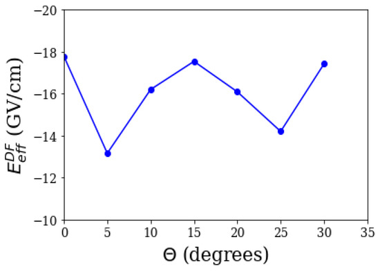
Figure 2.
The Dirac–Focl (DF) effective electric field vs .
6. Future Prospects
We shall now look at two of the many-body methods that we plan on implementing in the near future, due to their advantages over the conventional coupled cluster approach.
6.1. The Normal Coupled Cluster Method
In this variant of the coupled cluster method, the bra and the ket are defined on different footings [77], as
where
Here, s refer to the t amplitudes, and to the operators associated with particle-hole excitations. are the set of creation and annihilation operators, which are associated with de-excitations.
6.1.1. Amplitude Equations by Variational Principle
We can derive the amplitude equations for the normal coupled cluster method (NCCM), starting from the variational principle. Consider an energy functional, given by
According to the variational principle:
Using , we obtain:
In the second term on the left hand side, and can be switched, since they commute. Therefore,
6.1.2. The Expectation Value
Since the bra and the ket are treated differently, as seen earlier, the resulting NCCM expectation value expression naturally terminates. For any operator, , this can be seen as follows:
For illustration, let us consider NCCM in the singles and doubles approximation, that is, NCCSD. One can show that
Therefore,
terminates depending on the rank of , and therefore NCCM expectation value avoids the issue of truncation.
6.1.3. The Hellmann-Feynman Theorem
An important attribute of NCCM that makes it attractive, besides being variational and having an expectation value that naturally terminates, is that it satisfies the Hellman-Feynman Theorem (HFT), that is,
where is the Hamiltonian depending on a continuous parameter , is an eigen state of the Hamiltonian, and is the energy of the state .
For NCCM, the Hellmann-Feynman theorem takes the following form:
This expression can be rigorously proved. Expanding , and in the above equation, with , and equating the zeroeth powers of , we obtain
Here, and are the zeroth order or unperturbed parts of the wave functions for the bra and ket in lambda CC respectively. Therefore, the effective electric field could either be calculated as an expectation value, as shown earlier, or as an energy derivative, as shown above. For example, in a recent work, Sahoo and Das calculate the enhancement factors of the Hg atom using spherical symmetry to probe nuclear EDMs in the expectation value approach [78], while Sasmal et al. compute the effective electric field of RaF using the energy derivative approach [79]. We are planning on implementing the former and the extended coupled cluster method (ECCM) for our molecular calculations. In the ECCM, the same ket is used as in the NCCM, but the in the bra is replaced with [77].
6.2. The Analytical Derivative Approach
Following the approach by Monkhorst’s [80], we shall begin with the familiar equations from Section 4.5:
Also,
Starting from here, one can show that after some algebra and equating terms of the order lambda, the energy and amplitude equations can be obtained as
Therefore, one solves the coupled cluster equations, hence obtaining the t amplitudes, followed by solving for the amplitude equations given above to obtain . Finally, from the energy equation, one can evaluate . The effective electric field could thus be obtained, as it is a first order property.
Having introduced the two methods, we shall now compare them with the conventional coupled cluster approach. As seen earlier, the NCCM expectation value naturally terminates, unlike the CCM expression. Therefore, one expects NCCM to be more accurate (for a given level of particle-hole excitation and choice of basis), as it can capture missing correlation effects in CCM that arise as a consequence of manually terminating an infinite series. NCCM also satisfies the Hellmann-Feynman theorem. The analytical derivative approach recasts a property as an energy, and therefore there is no truncation involved in this method either, hence making this approach more accurate than CCM. We also note that the analytical derivative approach fares better than FFCC, since the latter involves running several calculations to obtain a property and also could have numerical issues. However, both NCCM and analytical derivative are harder to implement, and are computationally more expensive, as both require us to solve for an additional set of amplitudes. The NCCM treats the bra and the ket differently, and we need to evaluate the unperturbed bra and ket amplitudes, while in the analytical derivative approach, we need to solve for unperturbed and perturbed ket amplitudes. In CCM, one solves only for the unperturbed ket amplitudes. Also, using these methods for polyatomic systems is expected to be more challenging, and the degree of complexity could vary depending on factors such as the state of the molecule, and the number of valence electrons in that system.
7. Conclusions and Outlook
Relativistic many-body theory is indispensable in the searches of electron EDM. It is necessary to determine the upper limit for eEDM and also for identifying promising candidates for eEDM searches. With new results expected for the electron EDM experiments, improvements in relativistic many-body calculations in molecules are desirable. Relativistic coupled cluster theory is well suited for the calculations associated with eEDM searches mentioned above. It would be necessary to develop different variants of the theory for this purpose: normal CC method, the analytical derivative approach, ECCM [77,81], and tensor network tailored CC theory for open-shell molecules [82].
Author Contributions
All of the authors have contributed equally in the execution of the reported work. V.S.P. prepared the manuscript, B.P.D. supervised this review article, and the other co-authors were involved in discussing the manuscript.
Funding
Computations were performed on the CHIYO workstation at the Tokyo Institute of Technology, and vikram-100 cluster, at Physical Research Laboratory. M.A., A.S., and M.H. thanks JSPS KAKENHI Grant No. 17J02767, No. 17H03011, No. 17H02881, and No. 18K05040 for funding.
Conflicts of Interest
The authors declare no conflict of interest.
References
- Landau, L. On the conservation laws for weak interactions. Nucl. Phys. 1957, 3, 127–131. [Google Scholar] [CrossRef]
- Ballentine, L.E. Quantum Mechanics—A Modern Development; World Scientific Publishing: Singapore, 1998. [Google Scholar]
- Fortson, N.; Sandars, P.; Barr, S. The search for a permanent electric dipole moment. Phys. Today 2003, 56, 33–39. [Google Scholar] [CrossRef]
- Ibrahim, T.; Itani, A.; Nath, P. Electron electric dipole moment as a sensitive probe of PeV scale physics. Phys. Rev. D 2014, 90, 055006. [Google Scholar] [CrossRef]
- Fuyuto, K.; Hisano, J.; Senaha, E. Toward verification of electroweak baryogenesis by electric dipole moments. Phys. Lett. B 2016, 755, 491–497. [Google Scholar] [CrossRef]
- Luders, G. Proof of the TCP theorem. Ann. Phys. 2000, 281, 1004–1018. [Google Scholar] [CrossRef]
- Das, B.P.; Nayak, M.K.; Abe, M.; Prasannaa, V.S. Handbook of Relativistic Quantum Chemistry; Springer: Berlin/Heidelberg, Germany, 2015. [Google Scholar]
- Andreev, V.; Hutzler, N.R. Improved Limit on the Electric Dipole Moment of the Electron. Nature 2018, 562, 355–360. [Google Scholar]
- Cairncross, W.B.; Gresh, D.N.; Grau, M.; Cossel, K.C.; Roussy, T.S.; Ni, Y.Q.; Zhou, Y.; Ye, J.; Cornell, E.A. Precision measurement of the electron’s electric dipole moment using trapped molecular ions. Phys. Rev. Lett. 2017, 119, 153001. [Google Scholar] [CrossRef]
- Hudson, J.J.; Kara, D.M.; Smallman, I.J.; Sauer, B.E.; Tarbutt, M.R.; Hinds, E.A. Improved measurement of the shape of the electron. Nature 2011, 473, 493–496. [Google Scholar] [CrossRef]
- Kara, D.M.; Smallman, I.J.; Hudson, J.J.; Sauer, B.E.; Tarbutt, M.R.; Hinds, Ed.A. Measurement of the electron’s electric dipole moment using YbF molecules: Methods and data analysis. New J. Phys. 2012, 14, 103051. [Google Scholar] [CrossRef]
- Aggarwal, P.; Bethlem, H.L.; Borschevsky, A.; Denis, M.; Esajas, K.; Haase, Pi A.B.; Hao, Y.L.; Hoekstra, S.; Jungmann, K.; Meijknecht, T.B.; et al. Measuring the electric dipole moment of the electron in BaF. Eur. Phys. J. D 2018, 72, 197. [Google Scholar] [CrossRef]
- Vutha, A.C.; Horbatsch, M.; Hessels, E.A. Oriented polar molecules in a solid inert-gas matrix: A proposed method for measuring the electric dipole moment of the electron. Atoms 2018, 6, 3. [Google Scholar] [CrossRef]
- Vutha, A.C.; Horbatsch, M.; Hessels, E.A. Orientation-dependent hyperfine structure of polar molecules in a rare-gas matrix: A scheme for measuring the electron electric dipole moment. Phys. Rev. A 2018, 98, 032513. [Google Scholar] [CrossRef]
- Kozyryev, I.; Hutzler, N.R. Precision measurement of time-reversal symmetry violation with laser-cooled polyatomic molecules. Phys. Rev. Lett. 2017, 119, 133002. [Google Scholar] [CrossRef] [PubMed]
- Hoogeveen, F. DESY Reports, 006-90 (1990). Available online: https://lib-extopc.kek.jp/preprints/PDF/1990/9003/9003294.pdf (accessed on 10 June 2019).
- Pospelov, M.; Ritz, A. CKM benchmarks for electron electric dipole moment experiments. Phys. Rev. D 2014, 89, 056006. [Google Scholar] [CrossRef]
- Salpeter, E. Some atomic effects of an electronic electric dipole moment. Phys. Rev. 1958, 112, 1642. [Google Scholar] [CrossRef]
- Hunter, L.R. Tests of time-reversal invariance in atoms, molecules, and the neutron. Science 1991, 252, 73–79. [Google Scholar] [CrossRef] [PubMed]
- Schiff, L. Measurability of nuclear electric dipole moments. Phys. Rev. 1963, 132, 2194. [Google Scholar] [CrossRef]
- Abe, M.; Gopakumar, G.; Hada, M.; Das, B.P.; Tatewaki, H.; Mukherjee, D. Application of relativistic coupled-cluster theory to the effective electric field in YbF. Phys. Rev. A 2014, 90, 022501. [Google Scholar] [CrossRef]
- Das, B.P. Aspects of Many-Body Effects in Molecules and Extended Systems; Mukherjee, D., Ed.; Springer: Berlin, Germany, 1989; p. 411. [Google Scholar]
- Griffiths, D. Introduction to Quantum Mechanics, 2nd ed.; Pearson Education Limited: Essex, UK, 2014. [Google Scholar]
- Sucher, J. Foundations of the relativistic theory of many-electron atoms. Phys. Rev. A 1980, 22, 348. [Google Scholar] [CrossRef]
- Dyall, K.G.; Faegri, K., Jr. Introduction to Relativistic Quantum Chemistry; Oxford University Press: New York, NY, USA, 2006. [Google Scholar]
- Stanton, R.E.; Havriliak, S. Kinetic balance: A partial solution to the problem of variational safety in Dirac calculations. J. Chem, Phys. 1984, 81, 1910. [Google Scholar] [CrossRef]
- Bishop, R.F.; Kummel, H.G. The coupled-cluster method. Phys. Today 1987, 40, 52. [Google Scholar] [CrossRef]
- Bishop, R.F. Microscopic Quantum Many-Body Theories and Their Applications; Springer: Berlin, Germany, 1997. [Google Scholar]
- Kvasnicka, V.; Laurinc, V.; Biskupic, S. Coupled-cluster approach in electronic structure theory of molecules. Phys. Rep. 1982, 90, 159–202. [Google Scholar] [CrossRef]
- Cizek, J. Advances in Chemical Physics, Volume XIV: Correlation Effects in Atoms and Molecules; Lefebvre, W.C., Moser, C., Eds.; Interscience Publishers: New York, NY, USA, 1969. [Google Scholar]
- Shavitt, I.; Bartlett, R.J. Many Body Methods in Chemistry and Physics; Cambridge University Press: Cambridge, UK, 2009. [Google Scholar]
- Lindgren, I.; Morrison, J. Atomic Many-Body Theory, 2nd ed.; Springer: Berlin, Germany, 1986. [Google Scholar]
- Salter, E.A.; Sekino, H.; Bartlett, R.J.J. Property evaluation and orbital relaxation in coupled cluster methods. Chem. Phys. 1987, 87, 502–509. [Google Scholar] [CrossRef]
- Yanai, T.; Abe, M.; Hirata, S.; Iikura, H.; Inoue, H.; Kamiya, M.; Kawashima, Y.; Nakajima, T.; Nakano, H.; Nakao, Y.; et al. UTCHEM: A Program for ab initio Quantum Chemistry; Goos, G., Hartmanis, J., van Leeuwen, J., Eds.; Lecture Notes in Computer Science; Springer: Berlin, Germany, 2003; Volume 2660, p. 84. [Google Scholar]
- Yanai, T.; Nakajima, T.; Ishikawa, Y.; Hirao, K. A new computational scheme for the Dirac-Hartree-Fock method employing an efficient integral algorithm. J. Chem. Phys. 2001, 114, 6526–6538. [Google Scholar] [CrossRef]
- Abe, M.; Yanai, T.; Nakajima, T.; Hirao, K. A four-index transformation in Dirac’s four-component relativistic theory. Chem. Phys. Lett. 2004, 388, 68–73. [Google Scholar] [CrossRef]
- Visscher, L.; Jensen, H.J.A.; Saue, T.; Dubbilard, S.; Bast, R.; Dyall, K.G.; Ekström, U.; Eliav, E.; Fleig, T.; Gomes, A.S.P.; et al. DIRAC: A Relativistic Ab initio Electronic Structure Program, Release DIRAC08. 2008. Available online: http://www.diracprogram.org/ (accessed on 10 June 2019).
- Abe, M.; Prasannaa, V.S.; Das, B.P. Application of the finite-field coupled-cluster method to calculate molecular properties relevant to electron electric-dipole-moment searches. Phys. Rev. A 2018, 97, 032515. [Google Scholar] [CrossRef]
- Gomes, A.S.P.; Dyall, K.G.; Visscher, L. Relativistic double-zeta, triple-zeta, and quadruple-zeta basis sets for the lanthanides La-Lu. Theor. Chem. Acc. 2010, 127, 369. [Google Scholar] [CrossRef]
- Watanabe, Y.; Tatewaki, H.; Koga, T.; Matsuoka, O. Relativistic Gaussian basis sets for molecular calculations: Fully optimized single-family exponent basis sets for H–Hg. J. Comput. Chem. 2006, 27, 48–52. [Google Scholar] [CrossRef]
- Noro, T.; Sekiya, M.; Koga, T. Segmented contracted basis sets for atoms H through Xe: Sapporo-(DK)-nZP sets (n = D, T, Q). Theor. Chem. Acc. 2012, 131, 1124. [Google Scholar] [CrossRef]
- Sauer, B.E.; Cahn, S.B.; Kozlov, M.G.; Redgrave, G.D.; Hinds, E.A. Perturbed hyperfine doubling in the A2Π1/2 and [18.6]0.5 states of YbF. J. Chem. Phys. 1999, 110, 8424–8428. [Google Scholar] [CrossRef]
- Parpia, F.A. Ab initio calculation of the enhancement of the electric dipole moment of an electron in the YbF molecule. J. Phys. B 1998, 31, 1409. [Google Scholar] [CrossRef]
- Quiney, H.M.; Skaane, H.; Grant, I.P. Hyperfine and PT-odd effects in YbF. J. Phys. B At., Mol. Opt. Phys. 1998, 31, L85. [Google Scholar] [CrossRef]
- Titov, A.V.; Mosyagin, N.S.; Ezhov, V.F. P,T-Odd Spin-Rotational Hamiltonian for YbF Molecule. Phys. Rev. Lett. 1996, 77, 5346. [Google Scholar] [CrossRef] [PubMed]
- Nayak, M.K.; Chaudhuri, R.K. Ab initio calculation of P, T-odd effects in YbF molecule. Chem. Phys. Lett. 2006, 419, 191–194. [Google Scholar] [CrossRef]
- Gaul, K.; Berger, R. Zeroth order regular approximation approach to electric dipole moment interactions of the electron. J. Chem. Phys. 2017, 147, 014109. [Google Scholar] [CrossRef] [PubMed]
- Prasannaa, V.S.; Vutha, A.C.; Abe, M.; Das, B.P. Mercury monohalides: Suitability for electron electric dipole moment searches. Phys. Rev. Lett. 2015, 114, 183001. [Google Scholar] [CrossRef] [PubMed]
- Dyall, K.G. Relativistic and nonrelativistic finite nucleus optimized double zeta basis sets for the 4p, 5p and 6p elements. Theor. Chem. Acc. 1998, 99, 366–371. [Google Scholar]
- Schuchardt, K.L.; Didier, B.T.; Elsetha-gen, T.; Sun, L.; Gurumoorthi, V.; Chase, J.; Li, J.; Windus, T.L. Basis set exchange: A community database for computational sciences. J. Chem. Inf. Model. 2007, 47, 1045. [Google Scholar] [CrossRef] [PubMed]
- Knecht, S.; Fux, S.; van Meer, R.; Visscher, L.; Reiher, M.; Saue, T. Mössbauer spectroscopy for heavy elements: a relativistic benchmark study of mercury. Theor. Chem. Acc. 2011, 129, 631–650. [Google Scholar] [CrossRef]
- Cheung, N.-H.; Cool, T.A. Franck-Condon factors and r-centroids for the B2Σ-X2Σ systems of HgCl, HgBr, and HgI. J. Quant. Spectrosc. Radiat. Transfer 1979, 21, 397–432. [Google Scholar] [CrossRef]
- Meyer, E.R.; Bohn, J.L.; Deskevich, M.P. Candidate molecular ions for an electron electric dipole moment experiment. Phys. Rev. A 2006, 73, 062108. [Google Scholar] [CrossRef]
- Meyer, E.R.; Bohn, J.L. Prospects for an electron electric-dipole moment search in metastable ThO and ThF+. Phys. Rev. A 2008, 78, 010502. [Google Scholar] [CrossRef]
- Dmitriev, Y.Y.; Khait, Y.G.; Kozlov, M.G.; Labzovsky, L.N.; Mitrushenkov, A.O.; Shtoff, A.V.; Titov, A.V. Calculation of the spin-rotational Hamiltonian including P-and P, T-odd weak interaction terms for HgF and PbF molecules. Phys. Lett. A 1992, 167, 280–286. [Google Scholar] [CrossRef]
- Rennick, C.J.; Lam, J.; Doherty, W.G.; Softley, T.P. Magnetic trapping of cold bromine atoms. Phys. Rev. Lett. 2014, 112, 023002. [Google Scholar] [CrossRef] [PubMed]
- Hutzler, N.R.; Lu, H.I.; Doyle, J.M. The buffer gas beam: an intense, cold, and slow source for atoms and molecules. Chem. Rev. 2012, 112, 4803–4827. [Google Scholar] [CrossRef] [PubMed]
- Yang, Z.; Li, J.; Lin, Q.; Xu, L.; Wang, H.; Yang, T.; Yin, J. Laser-cooled HgF as a promising candidate to measure the electric dipole moment of the electron. Phys. Rev. A 2019, 99, 032502. [Google Scholar] [CrossRef]
- Dyall, K.G. Relativistic double-zeta, triple-zeta, and quadruple-zeta basis sets for the 4s, 5s, 6s, and 7s elements. J. Phys. Chem. A 2009, 113, 12638–12644. [Google Scholar] [CrossRef] [PubMed]
- Mestdagh, J.M.; Visticot, J.P. Semiempirical electrostatic polarization model of the ionic bonding in alkali and alkaline earth hydroxides and halides. Chem. Phys. 1991, 155, 79–89. [Google Scholar] [CrossRef]
- Ryzlewicz, C.; Törring, T. Formation and microwave spectrum of the 2Σ-radical barium-monofluoride. Chem. Phys. 1980, 51, 329–334. [Google Scholar] [CrossRef]
- Kozlov, M.G.; Titov, A.V.; Mosyagin, N.S.; Souchko, P.V. Enhancement of the electric dipole moment of the electron in the BaF molecule. Phys. Rev. A 1997, 56, R3326. [Google Scholar] [CrossRef]
- Nayak, M.K.; Chaudhuri, R.K. Ab initio calculation of P, T-odd interaction constant in BaF: a restricted active space configuration interaction approach. J. Phys. B 2006, 391231. [Google Scholar]
- Sunaga, A.; Prasannaa, V.S.; Abe, M.; Hada, M.; Das, B.P. Ultracold mercury-alkali-metal molecules for electron-electric-dipole-moment searches. Phys. Rev. A 2019, 99, 040501. [Google Scholar] [CrossRef]
- Dyall, K.G.; Gomes, A.S.P. Revised relativistic basis sets for the 5d elements Hf–Hg. Theor. Chem. Acc. 2010, 125, 97. [Google Scholar] [CrossRef]
- Dyall, K.G. Relativistic double-zeta, triple-zeta, and quadruple-zeta basis sets for the light elements H–Ar. Theor. Chem. Acc. 2016, 135, 128. [Google Scholar] [CrossRef]
- Thiel, L.; Hotop, H.; Meyer, W. Ground-state potential energy curves of LiHg, NaHg, and KHg revisited. J. Chem. Phys. 2003, 119, 9008–9020. [Google Scholar] [CrossRef]
- Park, J.W.; Yan, Z.Z.; Loh, H.; Will, S.A.; Zwierlein, M.W. Second-scale nuclear spin coherence time of ultracold 23Na40K molecules. Science 2017, 357, 372–375. [Google Scholar] [CrossRef]
- Hara, H.; Takasu, Y.; Yamaoka, Y.; Doyle, J.M.; Takahashi, Y. Quantum degenerate mixtures of alkali and alkaline-earth-like atoms. Phys. Rev. Lett. 2011, 106, 205304. [Google Scholar] [CrossRef]
- Hansen, A.H.; Khramov, A.Y.; Dowd, W.H.; Jamison, A.O.; Plotkin-Swing, B.; Roy, R.J.; Gupta, S. Production of quantum-degenerate mixtures of ytterbium and lithium with controllable interspecies overlap. Phys. Rev. A 2013, 87, 013615. [Google Scholar] [CrossRef]
- Kozyryev, I.; Baum, L.; Matsuda, K.; Augenbraun, B.L.; Anderegg, L.; Sedlack, A.P.; Doyle, J.M. Sisyphus laser cooling of a polyatomic molecule. Phys. Rev. Lett. 2017, 118, 173201. [Google Scholar] [CrossRef]
- Isaev, T.A.; Zaitsevskii, A.V.; Eliav, E. Laser-coolable polyatomic molecules with heavy nuclei. J. Phys. B 2017, 50, 225101. [Google Scholar] [CrossRef]
- Steimle, T. (Arizona State University, Tempe, AZ, USA). Private communication, 2018.
- Gaul, K.; Marquardt, S.; Isaev, T.; Berger, R. Systematic study of relativistic and chemical enhancements of P, T-odd effects in polar diatomic radicals. Phys. Rev. A 2019, 99, 032509. [Google Scholar] [CrossRef]
- Denis, M.; Haase, P.A.B.; Timmermans, R.G.E.; Eliav, E.; Hutzler, N.R.; Borschevsky, A. Enhancement factor for the electric dipole moment of the electron in the BaOH and YbOH molecules. arXiv 2019, arXiv:1901.02265. [Google Scholar] [CrossRef]
- Prasannaa, V.S.; Shitara, N.; Sakurai, A.; Abe, M.; Das, B.P. Enhanced sensitivity of the electron electric dipole moment from YbOH: The role of theory. arXiV 2019, arXiv:1902.09975. [Google Scholar] [CrossRef]
- Arponen, J. Variational principles and linked-cluster exp S expansions for static and dynamic many-body problems. Ann. Phys. (NY) 1983, 151, 311–382. [Google Scholar] [CrossRef]
- Sahoo, B.K.; Das, B.P. Relativistic Normal Coupled-Cluster Theory for Accurate Determination of Electric Dipole Moments of Atoms: First Application to the Hg199 Atom. Phys. Rev. Lett. 2018, 120, 203001. [Google Scholar] [CrossRef] [PubMed]
- Sasmal, S.; Pathak, H.; Nayak, M.K.; Vaval, N.; Pal, S. Relativistic coupled-cluster study of RaF as a candidate for the parity-and time-reversal-violating interaction. Phys. Rev. A 2016, 93, 062506. [Google Scholar] [CrossRef]
- Monkhorst, H.J. Calculation of properties with the coupled-cluster method. Int. J. Quant. Chem., Supplement: Proceedings of the International Symposium on Atomic, Molecular, and Solid state Theory, Collision Phenomena, and Computational Methods 1977, 12, S11. Available online: https://onlinelibrary.wiley.com/doi/abs/10.1002/qua.560120850 (accessed on 10 June 2019).
- Bishop, R.F. An overview of coupled cluster theory and its applications in physics. Theoret. Chim. Acta 1991, 80, 95–148. [Google Scholar] [CrossRef]
- Faulstich, F.M.; Laestadius, A.; Kvaal, S.; Legeza, O.; Schneider, R. Analysis of The Coupled-Cluster Method Tailored by Tensor-Network States in Quantum Chemistry. arXiv 2018, arXiv:1802.05699. [Google Scholar]

© 2019 by the authors. Licensee MDPI, Basel, Switzerland. This article is an open access article distributed under the terms and conditions of the Creative Commons Attribution (CC BY) license (http://creativecommons.org/licenses/by/4.0/).