Measurement of the Magnetic Field in a Linear Magnetized Plasma by Tunable Diode Laser Absorption Spectroscopy

Abstract

Tunable diode laser absorption spectroscopy (TDLAS) is a commonly used technique to measure the temperature and density of atoms or molecules in a gas. In this work, we demonstrate that the TDLAS diagnostics could be effectively applied to measure the magnetic field in a low-density weakly magnetized plasma using the Zeeman splitting of the absorption spectrum of lines from noble gases. The laser wavelength is tailored to fit the $1s_5\to 2p_6$ transition of atomic Ar with the wavelength $\lambda =763.51\mathrm{nm}$. Two mechanisms of line broadening and splitting are observed: Doppler broadening and Zeeman effect. The latter is especially pronounced by applying polarization-selective observation of the absorption to the TDLAS measurements. By fitting the $\sigma$ and $\pi$ components of the absorption spectrum, the line-integrated magnetic field on the order of 30–50 mT is determined. The agreement between the measured values and the vacuum field (neglecting the impact of the plasma) calculations on the axis of the PSI-2 is found to be about 15–20%.

1. Introduction

The measurement of the magnetic field in laboratory and astrophysical plasmas represents one of the most studied parameter in plasma physics, and at the same time is one of the most crucial parameters for steady-state plasma operation [1]. A variety of different techniques is used to determine the magnetic field. For instance, for laboratory plasmas the magnetic field can be obtained e.g., by optical emission spectroscopy (OES) by measuring the Zeeman splitting of an emission line [2,3], by Thomson scattering of laser light [4], by inductive sensors [5], or by accurate description of the line shapes of quasi-isotropic fields [6]. In interstellar plasmas, only OES can be used to determine magnetic fields due to the distance between plasma source and observer [7,8,9]. Especially the diagnostics that do not disturb the plasma are attractive. TDLAS is a widely and commonly used technique in physics to measure the density and temperature of atomic or molecular species in the plasma [10,11,12,13]. Zeeman splitting of TDLAS spectra was already reported before [14]; however, we are not aware of measurements of the magnetic field using a TDLAS system on metastable levels of noble gases.

The knowledge of the magnetic field is also important to measure the behavior of metastable levels of argon (Ar) in the linear plasma of PSI-2 [15,16]. Metastable Ar has a potential role in the excitation channel [17] of the emission of reflected hydrogen atoms at the plasma-surface interface. The current application and further development of the Doppler-shifted reflectance measurements (DSRM) diagnostic [18] in plasma cleaning discharges with electron temperature on the order of a few eV or less depends crucially on the answer to the following question: Are the metastable levels of Ar, in comparison with Kr or other noble gases, responsible for the strong emission of Balmer lines [19]? In this work, we demonstrate the first measurement of the magnetic field using tunable diode laser absorption spectroscopy (TDLAS) in the linear magnetized plasma of the PSI-2 device.

2. Materials and Methods

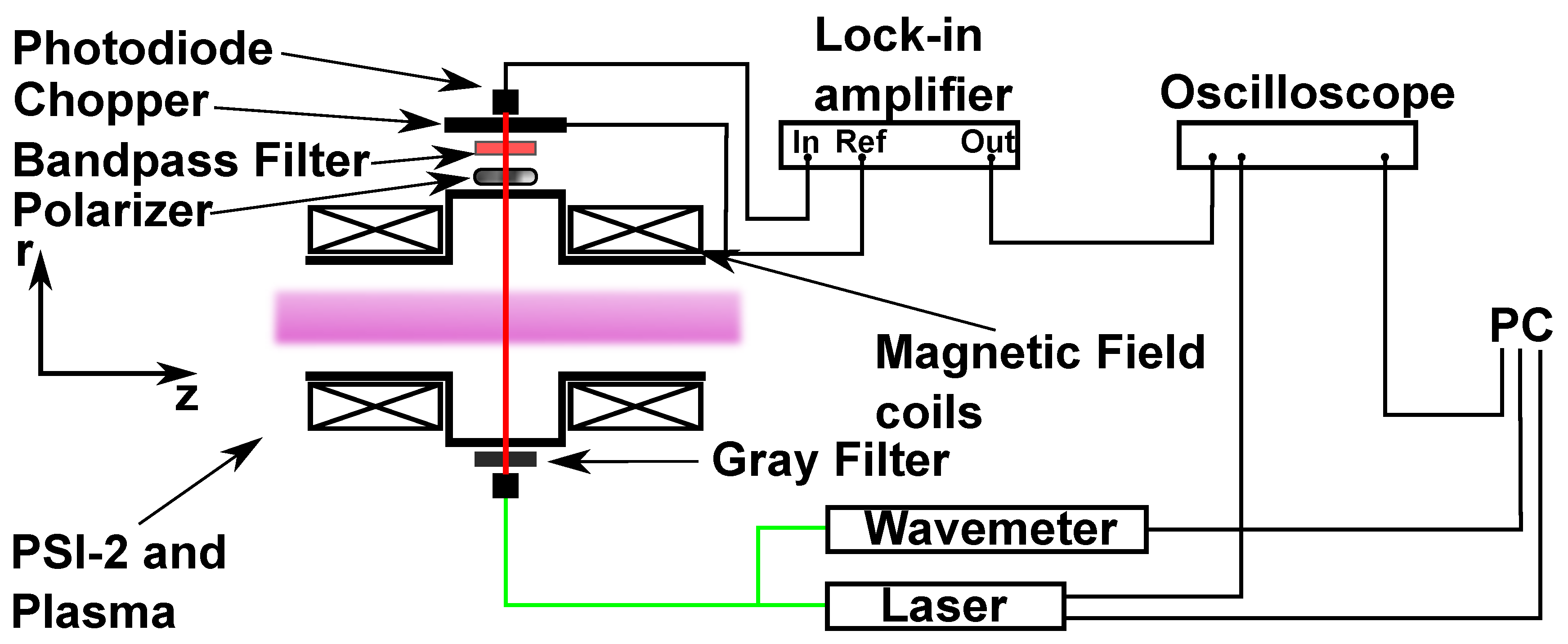
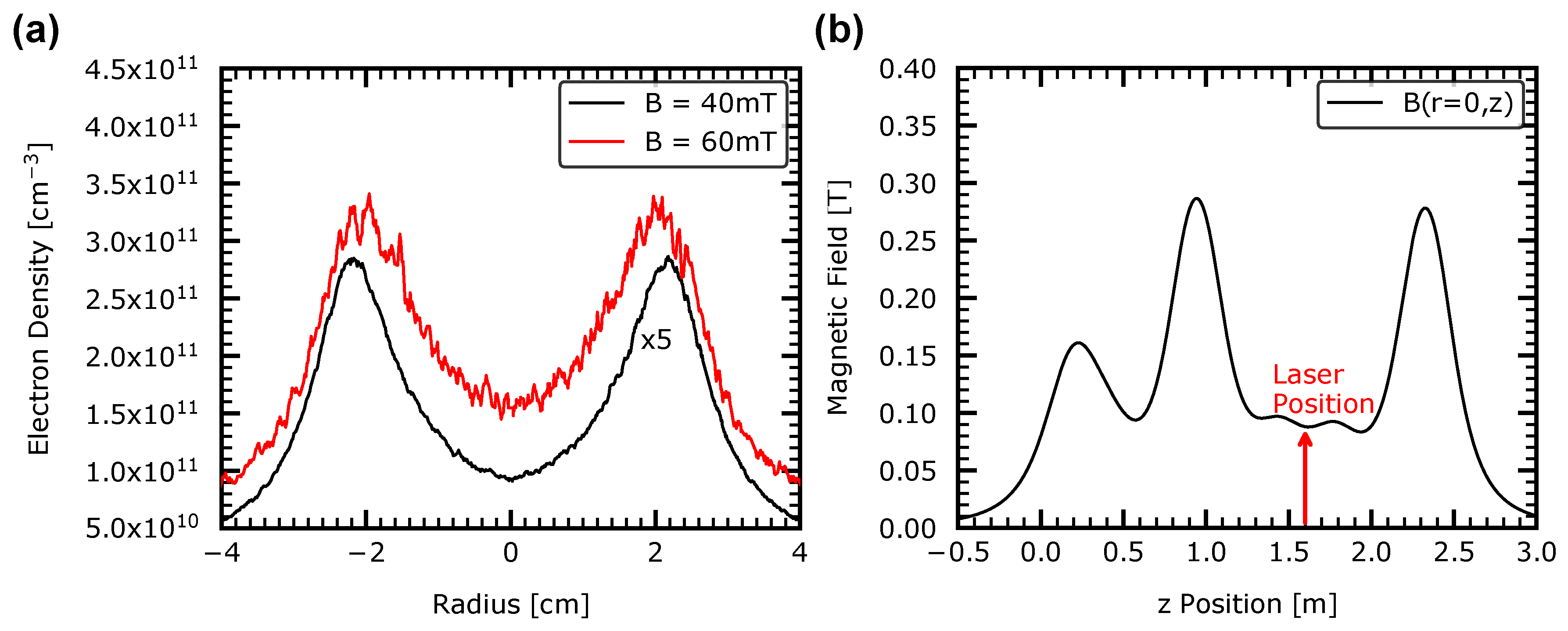
For the measurement of the transition, a TDLAS system is installed at the PSI-2, as shown schematically in Figure 1. The PSI-2 device has a hollow plasma profile with a cylindrical geometry that is a result of the source geometry. As an example of the plasma profile, the electron density for two magnetic field configurations is shown in Figure 2a. The laser beam path is positioned in a way that the absorption is measured through the center of the plasma column. The measurements were performed at a normal gas pressure between 0.01–0.02 Pa. The PSI-2 plasma is confined by six magnetic coils that produce a magnetic field in z-direction. A more detailed description of the PSI-2 device is given in [16]. The standard currents for the six coils are given in

Table 1. Geometry and standard settings of the magnetic coils of PSI-2 [20]. Note that coils 4 and 5 are connected in series.

Coil	1	2	3	4	5	6
$r_{min} \left[\mathrm{m}\right]$	$0.178$	$0.178$	$0.140$	$0.230$	$0.230$	$0.140$
$r_{max} \left[\mathrm{m}\right]$	$0.322$	$0.322$	$0.288$	$0.295$	$0.295$	$0.288$
$z_{min} \left[\mathrm{m}\right]$	$0.098$	$0.306$	$0.848$	$1.388$	$1.735$	$2.167$
$z_{max} \left[\mathrm{m}\right]$	$0.289$	$0.498$	$1.094$	$1.498$	$1.845$	$2.413$
winding N	600	600	335	81	81	335
$I_0 \left[\mathrm{A}\right]$	90	30	310	300	300	310

(values are taken from [20]). In the following, the standard current is shortened with $I_0$. The measurement is performed approx. 1.6 m away from the plasma source. At this position, the standard magnetic field can be calculated by the Biot–Savart law (Equation (1)) using the values given in Table 1: $B(r=0,z=1.6)=88 \mathrm{mT}$ [20].

$$\mathbf{B}\left(\mathbf{r}\right)={\displaystyle \sum _{i=1}^6}\int \frac{{\mu }_0}{4\pi }\frac{{\mathbf{j}}_i\times (\mathbf{r}-{\mathbf{r}}_i^{\prime })}{|\mathbf{r}-{\mathbf{r}}_i^{\prime }{|}^3}{d}^3{r}_i^{\prime },$$

(1)

where ${\mathbf{j}}_i$ is the current density of coil i and ${\mu }_0$ is the magnetic constant. The magnetic field along the z-axis is shown in Figure 2b. Two different magnetic field configurations were analyzed, namely $0.4I_0$ and $0.6I_0$, by varying the current in the coils. The Biot–Savart law describes the dependence of coil current and the magnetic field as linear. Thus the expected magnetic field should be $B\approx 35 \mathrm{mT}$ for $0.4I_0$ and $B\approx 53 \mathrm{mT}$ for $0.6I_0$.

The laser used in this experiment is a DLpro cw laser from Toptica (TOPTICA Photonics AG, 82166 Gräfelfing) with a nominal output power of $70 \mathrm{mW}$ at $763.5 \mathrm{nm}$ and a maximum current of 185 mA. The laser wavelength can be adjusted freely between 750 and 795 $\mathrm{nm}$, and a line width equals $110 \mathrm{kHz}$. During the measurement, the wavelength is scanned in a range of about $1 \mathrm{nm}$ with the frequency of $0.1 \mathrm{Hz}$ around a central wavelength by changing the grating position inside the laser. The grating is controlled by a piezo crystal. The laser beam is coupled into a single mode fiber and split up with a ratio of 99:1. One percent of the beam intensity is guided into a wavemeter (WS-6, produced by HighFinesse) for in situ wavelength monitoring. The precision of the wavemeter is $0.1 \mathrm{pm}$. The wavelength resolution of the TDLAS system is limited by the wavemeter. The other $99\%$ of the power is guided into the PSI-2 device using an additional $30 \mathrm{m}$ single mode optical fiber. The laser output power is measured with a power meter after the beam splitter and is determined to 10–20 $\mathrm{mW}$ by operating the laser at a current of $130 \mathrm{mA}$. The major power losses are due to the coupling between laser and fiber. Before the laser beam is guided into the PSI-2 device, a filter wheel with different gray filters is set into the optical path in order to control the laser power that is guided into the plasma. After the interaction with the plasma, a bandpass filter and a chopper wheel are positioned in the optical path. A polarization plate is also introduced between the vacuum window and the photo diode. The circular polarized $\sigma$ component ($\Delta m=\pm 1$) is observed using a linear polarizer with the axis being perpendicular to the z-axis of the PSI-2. The linear polarized $\pi$ component ($\Delta m=0$) is observed using the same linear polarizer with the axis being parallel to the z-axis of the PSI-2. The bandpass filter (Thorlabs FB760-10, CWL = $760\pm 2 \mathrm{nm}$, full-width-half-maximum (FWHM) = $10\pm 2 \mathrm{nm}$) is used to block the plasma radiation at all wavelengths except the laser wavelength of $763.5 \mathrm{nm}$. The chopper wheel chops the signal with a frequency of $1 \mathrm{kHz}$. The chopped beam intensity is measured with a photo diode (Thorlabs, PDA36A-EC-Si Switchable Gain Detector, 350–1100 $\mathrm{nm}$) right behind the chopper wheel. Then, it is converted into an electrical signal and analyzed with a dual lock-in amplifier (OrtoLock 9502). The linearity of the photo diode output signal was measured in the laboratory using the laser at a wavelength of $763.5106 \mathrm{nm}$ and a set of ND filters (Thorlabs FW212CNEB). The results of the measurements for different amplifications of the photo diode are shown in Figure 3. The linearity of the photo diode signal was demonstrated by changing the laser power from $6.1 \mathrm{mW}$ to $12 \mathsf{\mu }\mathrm{W}$. Only at low output signals below $100 \mathrm{mV}$, the photo diode demonstrated a higher signal, as expected. The results were confirmed by using three different sets of amplifications (40, 50, and $70 \mathrm{dB}$). 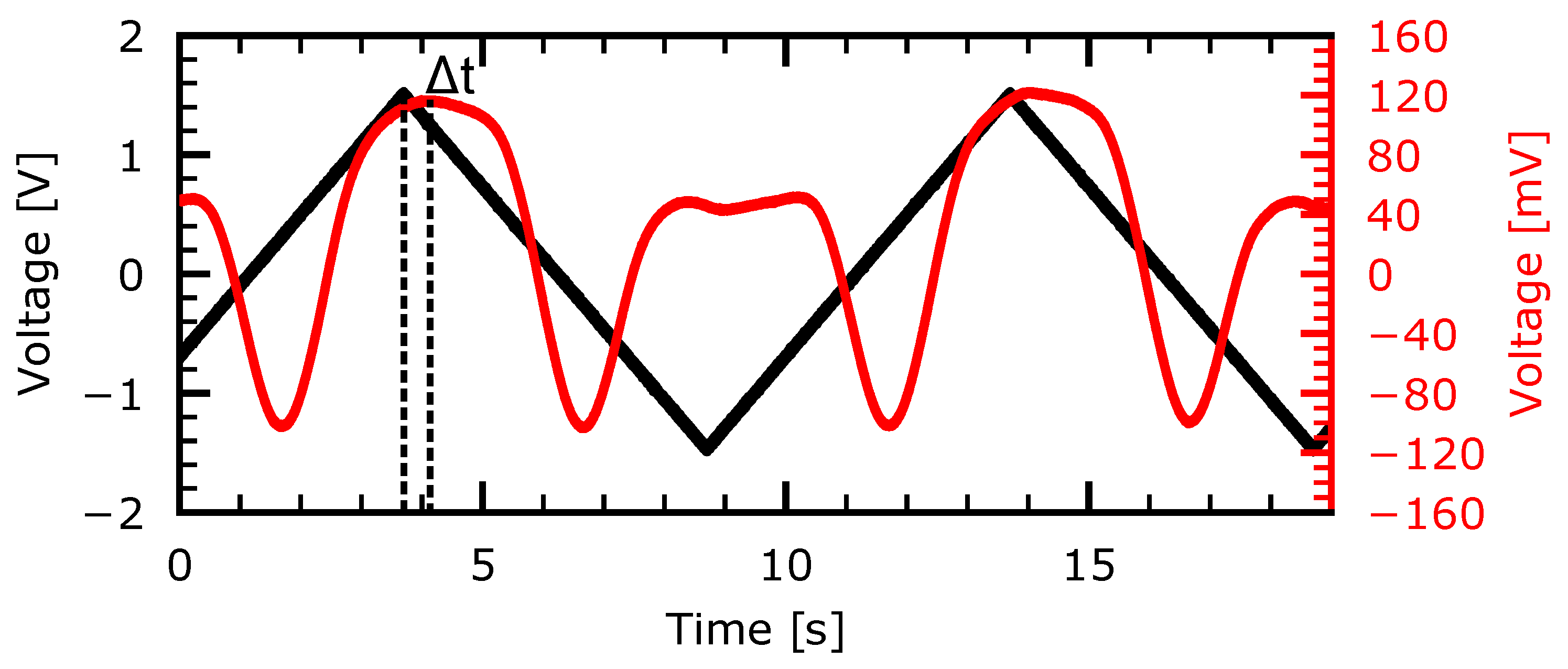For the $70 \mathrm{dB}$ gain, the signal was saturated for the filters with transmission above $50\%$ (1–4). For the reference signal of the lock-in amplifier, the frequency signal of the chopper wheel was used. The output of the lock-in amplifier as well as the voltage signal of the piezo crystal were measured with an oscilloscope (Figure 4). Together with the measured signal of the wavemeter, the x-axis of the oscilloscope can be recalculated in units of wavelength for further computation of the absorption signal. Note that due to the integration time of the lock-in amplifier, a time offset $\Delta t$ occurred between the absorption signal and the piezo voltage. The time offset $\Delta t$ ($\Delta t=300 \mathrm{ms}$) was corrected during the analysis of the spectrum. The ratio between the scanning period (5 s) and the integration time was 15, which should be sufficient to avoid large distortions in the obtained absorption line profile. For each spectrum, four different measurements were performed to eliminate the errors due to e.g., transmission losses in the optical path, as explained in detail in [11,12]:

• $L\left(\nu \right)$—Plasma on, Laser on
• $L_0\left(\nu \right)$—Plasma off, Laser on
• $P\left(\nu \right)$—Plasma on, Laser off
• $B\left(\nu \right)$—Plasma off, Laser off

The total transmittance of the signal can then be calculated (Equation (2)):

$$\frac{I\left(\nu \right)}{I_0\left(\nu \right)}=\frac{L\left(\nu \right)-P\left(\nu \right)}{L_0\left(\nu \right)-B\left(\nu \right)}$$

(2)

The experimental spectra shown in this work were calculated using only the measurements of $L\left(\nu \right)$ and $L_0\left(\nu \right)$. Furthermore, the spectra were corrected with regard to the linear background. The latter was induced by scanning the wavelength of the laser (see Figure 4).

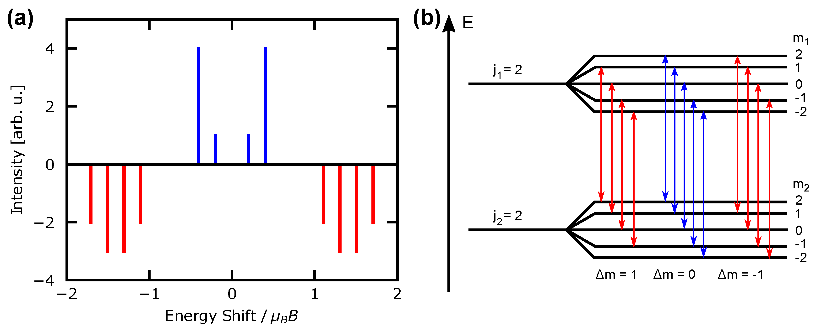
To calculate the magnetic field out of the absorption spectrum, the theoretical Zeeman spectrum of the line needs to be known. The laser wavelength is tailored for the transition from $1s_5(j_2=2)\to 2p_6(j_1=2)$ (the transition is given in Paschen notation). The relative intensities of the Zeeman lines $I_z$ (weak field) can be calculated using the Wigner 3-j symbols, assuming that all sublevels are equally populated [21]:

$$I_z\propto {\left(\begin{array}{ccc}{j}_1& 1& j_2\\ -m_1& m_1-m_2& m_2\end{array}\right)}^2,$$

(3)

where $j_1$ is the momentum quantum number of the upper level and $j_2$ of the lower level, and $m_1$ and $m_2$ are the corresponding magnetic quantum numbers. Possible transitions and the corresponding theoretical Zeeman pattern are shown in Figure 5. To fit the experimental spectrum, eight ($\sigma$ component) or five ($\pi$ component) Gaussian functions are used, each for one Zeeman component (note that the intensity of the Zeeman component of the transition $m_1=0\to m_2=0$ is 0):

$$I\left(\lambda \right)=\sum _i{A}_{i}exp\left(-\frac{{\left(\lambda -{\lambda }_i\right)}^2}{2{\sigma }_i^2}\right),$$

(4)

where $\lambda$ is the wavelength, $A_i$ is the amplitude, ${\lambda }_i$ is the center position, and ${\sigma }_i$ is the width of the Zeeman component i. All Zeeman components i are characterized by the same Doppler broadening, e.g., the temperature T, as a consequence of the constraint ${\sigma }_i={\sigma }_0$, is defined. Only the left component of Figure 5 (left) is fitted freely; for the other components, further constraints are defined. The amplitude of the Gauss functions is constrained by the ratio of the relative intensity given by Equation (3): $A_i=\frac{I_{z,i}}{I_{z,0}}{A}_0$, where $I_z$ is the theoretical relative intensity of the Zeeman pattern. The constraint for the central position follows from the energy-shift of the Zeeman splitting $\Delta E/E_0=\Delta \lambda /{\lambda }_0$, where $E_0$ and ${\lambda }_0$ are the energy or the wavelength of the field-free transition. The energy shift can be calculated as $\Delta E=(m_1{g}_1-m_2{g}_2){\mu }_{B}B$, where ${\mu }_B$ is the Bohr magneton and g is the Landé factor. The Landé factors are taken from the NIST database (for the upper level, $g_1=1.305$ and for the lower level, $g_2=1.506$) [22]. As a consequence, to fit the experimental data, only the amplitude $A_0$, the magnetic field B, and the temperature T are used as free parameters. For the temperature, the formula for Doppler broadening of spectral lines ${\lambda }_{1/2}^G={\lambda }_0\sqrt{8ln\left(2\right)\frac{kT}{M{c}^2}}$ is used [23] in SI units, where ${\lambda }_{1/2}^G$ is the full-width-half-maximum (FWHM) of the Gaussian function, ${\lambda }_0$ is the central wavelength of the line, k is the Boltzmann constant, T is the temperature of the light-absorbing species, M is the mass of the species, and c is the speed of light in vacuum. The FWHM of the Gaussian function can be calculated from $\sigma$ by ${\lambda }_{1/2}^G=2\sqrt{2ln\left(2\right)}\sigma$. Note that for the analysis of the absorption spectra, the hyperfine structure of Ar is neglected [24].

3. Results

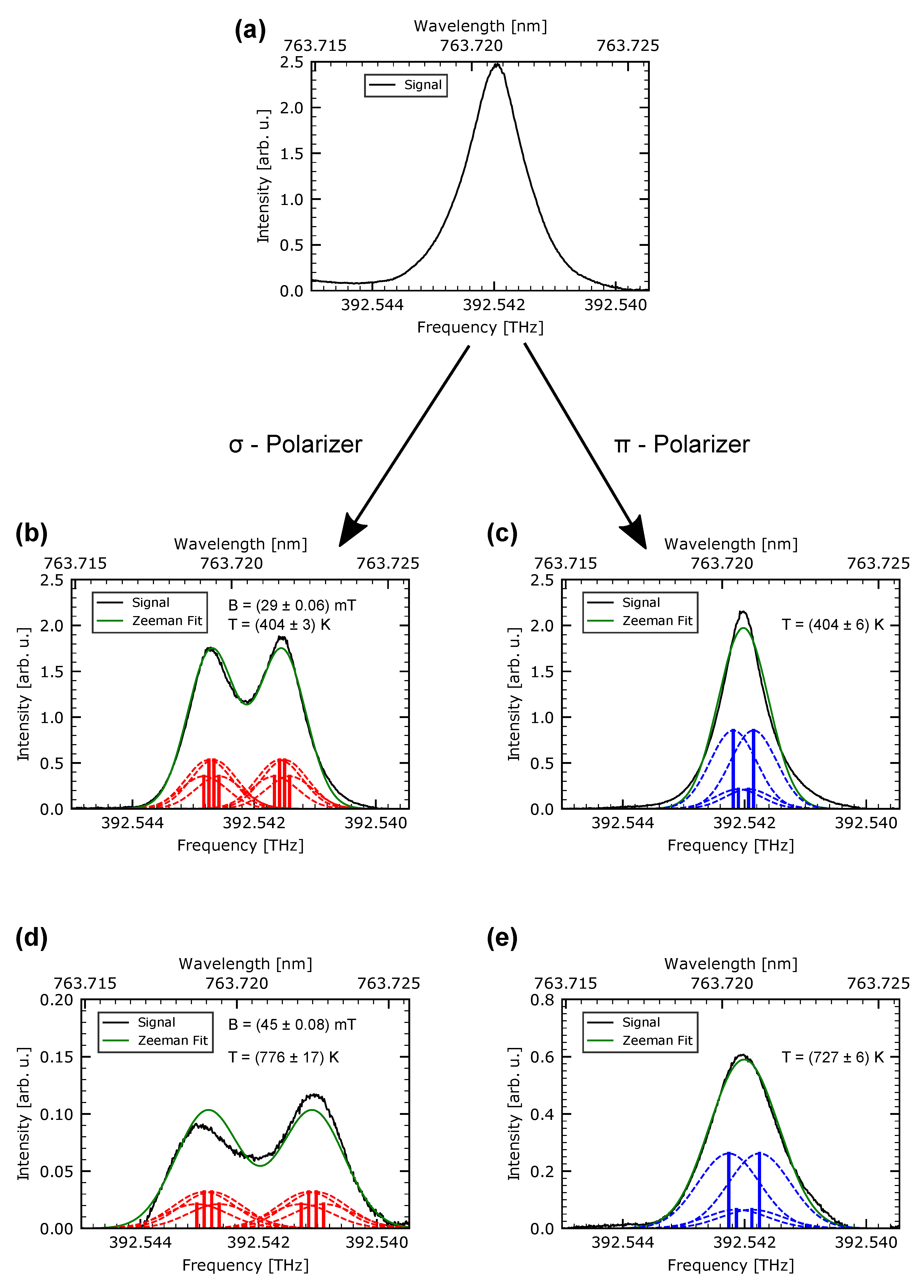
The following results were obtained by fitting the ratio $L\left(\nu \right)/L_0\left(\nu \right)$, as described in Section 2, either for the $\pi$ or the $\sigma$ component. We note that the obtained absorption spectra and results are line-integrated, and the magnetic field varies as a function of the position on the z-axis in the PSI-2. In Figure 6a, the obtained ratio $L\left(\nu \right)/L_0\left(\nu \right)$ at a magnetic field configuration of $I=0.4I_0$ is plotted. The measurement was performed without a polarization filter, thus the Zeeman splitting was not visible. However, when a polarization filter in front of the photo diode (Figure 1) was used, the observed signal split up into a $\sigma$ (Figure 6b) and a $\pi$ component (Figure 6c). The $\sigma$ spectrum was obtained by adjusting the polarizer in a perpendicular direction to the z-axis of the PSI-2 and showed two absorption peaks, whereas the $\pi$ spectrum where the polarization direction was adjusted parallel to the z-axis of the PSI-2 showed only one peak of absorption. This figure demonstrates the strong impact of the Zeeman effect on the line shape of the Ar I line. Neglecting the Zeeman effect in the PSI-2 for noble gases such as Ne, Ar, or Kr results in an overestimation of the derived gas temperature if the Zeeman effect is comparable or even larger than the Doppler broadening. In comparison to that for H or D lines, the Zeeman effect produced at most $10\%$ of the line width. Thus, for H or D lines in the PSI-2 device, the influence of the Zeeman effect on the determination of the temperature is negligible [19].

The $\sigma$ spectrum was fitted as explained in Section 2, where the magnetic field B was used as one fit parameter. The splitting for the $\sigma$ component consisted of eight instead of four components ($\pi$ component), and the splitting was larger, which reduced the errors of the fit considerably. The ratio $L\left(\nu \right)/L_0\left(\nu \right)$ is depicted in black, the green curve shows the fitted spectrum, and the red or blue dashed lines are single $\sigma$ or $\pi$ components. To fit the $\pi$ component, the obtained magnetic field of the $\sigma$ component was used and held constant. The temperature of both fits was compared to validate the fit of the $\pi$ component. Both components can describe the observed absorption spectrum well. The obtained magnetic field for the $0.4I_0$ setup was $B=(29\pm 0.06) \mathrm{mT}$, which is a deviation of $6 \mathrm{mT}$ from the expected value of $35 \mathrm{mT}$. For the case of $0.6I_0$, the obtained magnetic field was $B=(45\pm 0.08) \mathrm{mT}$, which deviates by $8 \mathrm{mT}$ from the expected value of $53 \mathrm{mT}$. The neutral gas temperature for $0.4I_0$ was determined to be $T_{Ar}=(404\pm 3) \mathrm{K}$ ($\sigma$ component) and $T_{Ar}=(404\pm 6) \mathrm{K}$ ($\pi$ component), and for $0.6I_0$, $T_{Ar}=(776\pm 17) \mathrm{K}$ ($\sigma$ component) and $T_{Ar}=(727\pm 6) \mathrm{K}$ ($\pi$ component). The errors for magnetic field B and temperature T were taken from the fitting routine.

4. Discussion

It is the first time that the TDLAS diagnostic is used to measure the magnetic field in a low density plasma. As described in Section 2, the transition $1s_5(j_2=2)\to 2p_6(j_1=2)$ of metastable Ar is used for the experiments. The fits are in good agreement with the experimental data. It is observed that an increase of the magnetic field by 50% leads to an increase in the splitting. The small asymmetry in the absorption spectrum (e.g., Figure 6) cannot be described by the fit because a symmetrical line profile is demanded. The asymmetry could be partially caused by the non-linear background of the obtained data but also the additional contribution of the charge-exchange between Ar ions and neutrals. The experimentally determined magnetic fields are systematically lower, and the discrepancy between the expected values in vacuum and those obtained experimentally is around $15\%$. Considering that a number of effects for the calculation of the theoretical value of the magnetic field are not considered, the agreement is rather good. On the one hand, the most probable reason for lower measured magnetic field values in comparison to the vacuum calculation is the collective motion of ions in the angular direction, which produces a magnetic field in the opposite direction compared to the external applied magnetic field. On the other hand, the obtained values of the magnetic field are derived from the line-of-sight integrated signal. The experimental values have to be analyzed for different lines-of-sight to derive the dependence on the observation angle. Eventually, using Abel inversion to obtain spatially resolved profiles of the magnetic field could lead to a better agreement. This will be investigated in the near future. In addition to the magnetic field, the temperature of the metastable Ar atoms was also determined. For the magnetic field of 35–53 $\mathrm{mT}$, the gas temperature was found to be around 400–800 $\mathrm{K}$. The comparison between the obtained temperature of the $\sigma$ and $\pi$ components shows that the temperatures are in the same order of magnitude, which validates both the magnetic field and the temperature determination. The two-fold increase in the gas temperature with magnetic field strength is probably related to an increase of the plasma density by a factor of five, as obtained by Langmuir probe measurements (Figure 2a). The TDLAS measurements provide data not only for magnetic field measurements, but also for gas rotation. Therefore, the integration time of the lock-in amplifier must be taken into account by analyzing the plasma rotation. For instance, the integration time of $300 \mathrm{ms}$ for the lock-in amplifier at the scanning time of $10 \mathrm{s}$ (Figure 4) results in a measured velocity of the atoms on the order of $0.5 \mathrm{km}/\mathrm{s}$. The wavelength calibration using an Ar lamp could be the most reliable solution to define the optimal integration time of the lock-in amplifier. Furthermore, the optical thickness of the absorption measurements was not analyzed. However, due to the weakening of the laser beam and the relatively low values of absorption, this effect is not expected to be significant under our conditions. The question about the optical thickness could be partially answered by also monitoring the intensity of other Ar I lines, such as $800.6157 \mathrm{nm}$, originating from the upper level of the absorption transition. Moreover, the experimental data will be extended by performing a radial scan of the plasma and compare the emission and absorption spectra of Ar at different experimental conditions. Finally, the TDLAS diagnostic could help to identify the density of metastable levels of Ar and their role in the plasma–solid interaction.