Abstract
In fluid turbulence, intermittency is the emergence of non-Gaussian tails in the distribution of velocity increments in small space and/or time scales. Intermittence is thus expected to gradually disappear as one moves from small to large scales. Here we study the turbulent-like intermittency effect experimentally observed in the distribution of intensity fluctuations in a disordered continuous-wave-pumped erbium-doped-based random fiber laser with specially-designed random fiber Bragg gratings. The intermittency effect is investigated as a crossover in the distribution of intensity increments from a heavy-tailed distribution (for short time scales), to a Gaussian distribution (for large time scales). The results are theoretically supported by a hierarchical stochastic model that incorporates Kolmogorov’s theory of turbulence. In particular, the discrete version of the hierachical model allows a general direct interpretation of the number of relevant scales in the photonic hierarchy as the order of the transitions induced by the non-linearities in the medium. Our results thus provide further statistical evidence for the interpretation of the turbulence-like emission previously observed in this system.
1. Introduction
The basic components of a conventional laser are an optical gain medium and an optical cavity. In such a laser, light can be generated by optically or electrically pumping the gain medium, where spontaneous emission occurs as a consequence of external excitation. The cavity, normally formed by mirrors, defines spatial modes and provides radiation feedback to the gain medium. Then, due to stimulated emission, light is amplified in the optical modes defined by the laser cavity. Above a certain pumping threshold, the overall gain of such photonic system overcomes its overall losses and laser radiation can be produced as a bright directional output beam. On the other hand, a random laser (RL) is a system which provides laser-like radiation but doesn’t rely on fixed mirrors, or a cavity, to provide optical feedback. This is achieved by exploring a multiple scattering mechanism, usually incorporated in the gain medium itself, which extends to the optical path of photons created by spontaneous emission inside the gain medium. This leads to an enhanced amplification of the emitted light due to stimulated emission, in a process called amplified spontaneous emission. As a result of the predominantly multimode character of the radiation emitted by a RL, its coherence properties are poorer than for a conventional laser. Besides this, there is strictly no light beam produced, as in a conventional laser. However, the intensity of the light coming out of a RL is still high, and these optical characteristics are useful for a myriad of applications. In imaging, the low spatial coherence results in the production of speckle patterns with lower visibility, and RLs can be used for producing smoother images [1]. The low temporal coherence makes RLs attractive for applications in optical coherence tomography, since for this imaging technique the shorter the light source coherence length, the better [2]. In diagnostics, the morphological change of a healthy, non scattering tissue, for example due to neoplasia, can lead to a tissue roughness capable of scattering light, and thus monitoring RL action in tissues can be an indication of several diseases [3].
From the point of view of basic science, photonics-based devices and processes have been exploited as important platforms for the observation of complex phenomena, such as turbulence [4] and spin glass [5,6], which have counterparts in natural events. Turbulence in photonics has been observed, for instance, in a Raman fiber laser [7] with a 770 m long highly dispersive fiber at 1550 nm, placed between two custom-designed fiber Bragg gratings (FBG) acting as the cavity mirrors. More recently, a turbulence-like hierarchy phenomenon has been demonstrated in a random fiber laser (RFL) [8], which differs from a conventional fiber laser in that the feedback is not provided by two static mirrors or two FBG but, instead, it arises from the multiple scattering of photons in a disordered medium. It thus forms an open complex disordered nonlinear system, which in the presence of gain leads to laser emission [9].
In Kolmogorov’s statistical approach to fluid turbulence, two concepts stand out: energy cascade and intermittency [10]. The energy cascade is the mechanism by which energy is transferred from large to small scales, thus creating a dynamical hierarchy. On the other hand, intermittency is the tendency of the distribution of velocity increments to develop heavy non-Gaussian tails. The intermittency effects are expected to fade away as we move from small to large scales. Here we complement our previous work on the hierarchical structure of the photonic turbulent regime observed in this RFL [8] by investigating the intermittency properties. In the photonic context, intermittency is characterized by the emergence of non-Gaussian tails in the distribution of increments of intensity in output spectra separated by short time scales. In this work, we show that intermittency gradually disappears as larger time separations between spectra are considered, yielding in this case a non-turbulent state with Gaussian distribution of intensity increments for large time scales. Our experimental results are theoretically supported by a hierarchical stochastic model that incorporates Kolmogorov’s theory of turbulence. In particular, by means of a discrete version of the hierarchical model we provide a general direct interpretation for the number of relevant scales in the photonic hierarchy as the order of the transitions induced by the non-linearities in the medium.
The RFL employed in this work is based on a specially-designed random FBG inscribed in an erbium (Er)-doped optical fiber, which is pumped by a continuous wave (CW) semiconductor laser. Thanks to the huge amount of emission spectra recorded—150,000—in the situations well below, near and well above threshold, this system could be characterized in detail and used to demonstrate photonic spin-glass behavior and Lévy-like statistics [11,12].
2. Results
2.1. Experimental Results
A home-assembled CW semiconductor pump laser operating at 1480 nm delivering up to 150 mW was used as optical pump for the Er-RFL, a polarization-maintaining Er-doped fiber (CorActive, peak absorption 28 dB/m @ 1530 nm, NA = 0.25, mode field diameter 5.7 m), in which the randomly distributed phase error grating was written [13], which acted as the scatterers. Using this procedure, improved randomness was achieved due to the very high number of scatterers (≫1000) implemented. For the present work, a fiber length of 30 cm was used and the measured threshold at 1480 nm CW pump was mW. Output powers of ∼1–2 mW were obtained for input powers ∼50–70 mW, a comfortable range for the measurements. The resolution-limited (by our instrument) Er-RFL linewidth was 0.2 nm. However, the number of longitudinal modes in the Er-RFL, measured using a speckle contrast technique, was found to be ∼200, thus demonstrating the longitudinal multimode character of the Er-RFL system [12]. The system Er-doped fiber plus CW pump laser was assembled along with input/output couplers to collect and analyze the emitted light.
The experimental observation of turbulent behavior in the Er-RFL system was obtained from the measurement of the output intensity fluctuations in a sequence of 150,000 emission spectra collected for three values of the excitation power P, namely below, near, and above the laser threshold [8]. The spectra for each excitation power were acquired with integration time ms.
Figure 1 displays the linewidth narrowing (blue) and emitted intensity (red) as a function of normalized excitation power , from which the RFL threshold can be clearly identified [11,12]. It is important to remark that the intensity fluctuations of the RFL system do not follow the pattern of those of the semiconductor pump laser, as evidenced from the comparative measurements of the standard deviation of maximum intensity for the pump laser and RFL, reported in [11,12]. Indeed, at excitation powers above the threshold the standard deviation (normalized by the average value of the maximum intensity) of the pump laser remained always close to zero, whereas that of the RFL reached values up to ∼ [11,12].
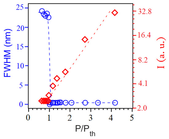
Figure 1.
Linewidth narrowing (blue) and emitted intensity (red) of the random fiber laser (RFL) system as a function of normalized excitation power . The evident change of behavior in both measurements identifies the RFL threshold. The measured threshold value was mW [11,12].
We display in Figure 2 a sample of 500 emission spectra (out of the whole set of 150,000 spectra) at each excitation power below [(a) ], near [(a) ], and above [(a) ] the RFL threshold [11,12].
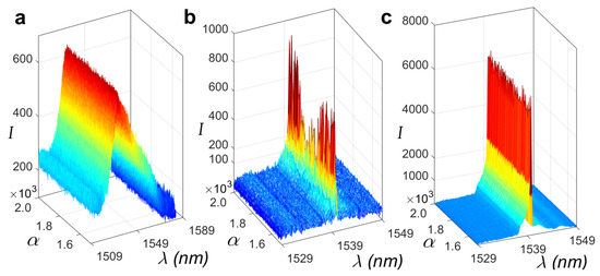
Figure 2.
Plots of 500 emission spectra at each excitation power below [(a) ], near [(b) ], and above [(c) ] the RFL threshold [11,12]. Intensity fluctuations are quite more intense near the threshold, if compared to those observed below and above. The value was chosen for the present analysis.
The spectra were obtained using a spectrometer with a liquid-N cooled infrared CCD camera providing a nominal 0.2 nm resolution at 1530.0 nm. We comment that the spectra peak at 1540.0 nm. It is noticeable that the intensity fluctuations below and above the threshold behave quite differently from those around the threshold. In particular, the special value was chosen for the analysis in this work, since in this regime the RFL system presents the coexistence of photonic turbulent and spin glass behaviors [8,14].
2.2. Theoretical Background
Our basic hypothesis is that the probability distribution of the experimental signal (see below) is a Gaussian at a local level (in time), with a slowly fluctuating variance . This means that we can write the signal’s local equilibrium distribution as a conditional Gaussian: . The marginal distribution is then obtained by compounding this local Gaussian with a background distribution of the fluctuating variance, thus
with being determined by the underlying turbulent dynamics. There are two universality classes of such models [15,16]: In one class has a power-law tail and in the other it shows a stretched-exponential behavior. Our experimental data is well fitted using the stretched-exponential class, and so we restrict the discussion to this case.
In fluid turbulence, the relevant statistical quantities (the signal) are the velocity increments between two points in the flow. By analogy, in photonic turbulence we may consider intensity increments between successive optical spectra,
with (shortest separation time scale between the spectra ) and k denotes the wavelength index. Thus, the object of our statistical analysis is the intensity increments between RL emission spectra and , always measured for the same wavelengths k in the spectra and . In the prelasing regime (), in which nonlinearities are irrelevant, the intensity increments are statistically independent and the probability distribution for a given wavelength, , , is a Gaussian. In contrast, when the excitation power is increased beyond the threshold, it has been shown in [8] that nonlinearities give rise to a turbulent emission in which the Gaussian form of the intensity increments distribution remains valid only at a local level, with a slowly fluctuating variance , for . Therefore, the local conditional distribution at the shortest time scale, , can be written for as
As pointed out above, in the statistical description of turbulence the non-Gaussian global form of can be obtained by compounding the above local Gaussian with a background distribution of variance fluctuations . Therefore, we may rewrite Equation (1) as
The complex dynamics (intermittency) of the turbulent state is thus captured by the background density and deriving it from a suitable statistical model is our next step.
2.2.1. Stochastic Model (H-Theory)
One important feature of the hierarchical multiscale theory of complex systems, the H-Theory [15,16], is that it allows to obtain an exact expression for the background density from the stationary solution of a set of stochastic differential equations that incorporates Kolmogorov’s hypothesis of turbulent cascades [15,16],
for , where N denotes the number of relevant intensity fluctuation time scales in the background variables. In our notation, the N-th hierarchy is assigned to the shortest time scale , that is, . The variable represents the fluctuating variance parameter at the respective scale in the hierarchy, with as the largest-scale average, and denote positive constants, and are independent Wiener processes. The first term in Equation (5) describes the deterministic coupling between adjacent scales, which leads to the relaxation towards , whilst the second term accounts for the non-linear couplings with the background variables at all scales, setting the ultimate source of intermittency. We remark that the form of these equations is dictated by the invariance under the scale transformation , along with the positivity requirement , , and some constraints on the moments of the stationary distribution [15,16].
Under the assumption of large time scales separation, , we write the density at the shortest scale as
where the conditional probability distribution arises from the stationary solution of Equation (5) in the form of a gamma density,
with . Remarkably, the multiple integral in Equation (6) has an analytical representation in terms of a Meijer G-function [17] which, with the use of the notation , is expressed as
where and we have introduced the vector notation and Since the first lower index of the Meijer G-function in Equation (8) is null, the parameters in the top row are not present, as indicated by the dash.
Finally, by substituting Equation (3) into the superposition integral (4), we obtain
which, by using Equation (8), allows the distribution of intensity increments at the shortest scale to be obtained explicitly,
We remark that the large- asymptotic limit of Equation (10) has the form of a heavy-tailed modified stretched exponential [17],
where , thus displaying important deviations from the Gaussian density, as expected for the photonic turbulent behavior of the short-scale distribution of intensity increments.
We also comment that when the empirical data contains some internal structure indicating the presence of clusters of statistically independent samples, it is sometimes useful to employ a more general family of distributions given by a discrete statistical mixture of multiscale distributions,
where the statistical weights satisfy and each is obtained from Equation (10) for the same number N of hierarchy scales and a specific set of internal parameters. In particular, in Reference [8] we apply the statistical mixture of two components ( in Equation (12)) to successfully explain all experimental results related to the turbulent laser emission in the RFL system.
2.2.2. Discrete Hierarquical Model
Although the dynamical stochastic model described above allows for a clear connection with fluid turbulence, it does not provide a direct interpretation of the discrete parameter N, i.e., the number of levels or relevant scales in the model hierarchy. In other words, it is not always clear which structure should play the role of the turbulent eddies in the complex dynamical system described by the H-theory, particularly in the photonic context. In order to address this issue, we introduce below a discrete model that makes direct contact with the central limit theorem (CLT) and provides a simple interpretation for the number N of hierarchical levels present in H-theory. A related approach, albeit restricted to the cases and of a two-dimensional random walk, can be found in Reference [18].
We start by defining X as a random variable, with denoting a set of M independent realizations of X. We also define the random variable Z via , and let . Then, the characteristic functions of and Z are related as follows:
In the standard form of the CLT, we consider M to be a large number, so that
where is the root-mean-square deviation of X. This characteristic function implies that is also Gaussian distributed, as expected from the CLT.
Let us now consider that M is a discrete random variable with probability . In this case, we may define a weighted averaged characteristic function,
Below we proceed by selecting from particular stationary solutions of well-known discrete stochastic processes. From these results, we will be able to make contact with the H-theory and the associated interpretation of the number of hierarchy scales N in the case of photonic turbulence in the RFL system.
(i) Poisson process ()
The Poisson process is described by the following master Equation [19],
which represents an interaction-free evolution in discrete space, with and a positive parameter. The solution is given by
where and the characteristic function is given by . If we rescale and take , we recover the expected result of the CLT, .
(ii) Pauli process ()
The master equation of the Pauli process is defined as [19]
where and , with being positive constants. The Pauli process contains dipole transitions [19], and its stationary solution reads , where and . The characteristic function is
Following the steps as in the previous case, if we rescale and take , we obtain
The corresponding distribution for the variable Y is thus
which is a particular case of Equation (10).
(iii) Negative binomial process ()
The negative binomial process is a generalization of the Pauli process that allows for the presence of bunches in the evolution of [19]. In this case, the stationary solution is
where and the parameter is the number of degrees of freedom. Notice that the binomial coefficient counts the number of partitions of M among states. The characteristic function reads
If we now rescale and take , we obtain
The corresponding distribution for the variable Y is
which is also a particular case of Equation (10). Notice that for we recover the results of the Pauli process.
We are now in position to state the general result for N arbitrary as follows. Consider a stochastic process with stationary distribution given by
where and . The integer parameter N gives the order of the transitions induced by the interactions described by the evolution of . In other words, there exists a non-vanishing coupling between and in the master equation. Observe that for (no correlations) and (dipole transitions) we recover the Poisson and negative binomial distributions, respectively. The corresponding distribution for the variable Y can be expressed as
which reproduces the exact stationary solution (10) of H-theory.
We can now interpret the parameter N in the H-theory description of photonic turbulence. In this context, if we consider to be a sum of M independent sources that contribute to the observed intensity increments and admit that M is proportional to the number of photons contributing to the photonic turbulent emission, then N might be understood as giving the order of the transitions induced by the non-linearities in the medium. Therefore, for the conventional coherent light of a laser one has , which implies a Gaussian distribution for the intensity increments. On the other hand, we may assign for chaotic light and for generic turbulent emission, which implies Equation (10) for the corresponding intensity increments distribution, in agreement with the results on the RFL photonic turbulent state reported in [8].
2.3. Intermittency in RFL Turbulent Emission
In fluid turbulence, intermittency is usually explained as being caused by fluctuations in the energy transfer rates or energy fluxes between adjacent scales and its detailed description is one of the goals of current research. A universal feature of intermittence is that its effect vanishes monotonically as we move from small to large scales. We shall verify this universal property in the RFL photonic turbulent state presented below.
We start the analysis by generating a matrix from the large dataset of intensity measurements at the excitation power , for (= 150,000) output spectra replicas (matrix rows) and 512 wavelengths indexed by k in the interval [1489.0 nm, 1591.4 nm] (matrix columns). We then perform a subtraction of replicas (rows) separated by units of time. In other words, we work with one intensity dataset for each wavelength indexed by k (i.e., for each column of the matrix), and also calculate the average over replicas (rows) for each k. In this procedure (see also Materials and Methods), each new matrix generated as above contains (150,000 − ) rows and 512 columns. We then perform the calculation of the distribution of the variable
for each given choice of measured at the wavelength 1539.8 nm around the peak emission (value of k corresponding to the matrix column 254).
Plots of such distributions are shown in Figure 3 [(a,b) ; (c,d) and (e) ]. In all cases, we notice an excellent agreement between the theoretical and experimental results for all values of . By applying the numerical procedure described above (see also Materials and Methods), we obtain a statistical mixture, defined as , where is given by (10) with fitting parameters , and . For the separation time between the RFL emission spectra, the distributions [(a)] and [(b)] with the best fit parameters , , , , and . On the other hand, for , the plots of [(c)] and [(d)], obtained for , , , , and . Remarkably, the results for a large separation in time [(e)] display the Gaussian profile of , in analogy to the nonturbulent pattern observed from the velocity increments of rather distant points in a turbulent fluid.
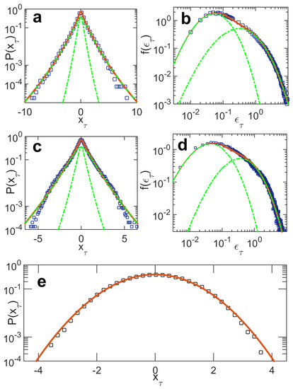
Figure 3.
Distributions of intensity increments and background density for RFL emission spectra separated by units of time that are (a,b) first neighbors , (c,d) second neighbors , and (e) distant neighbors . The theoretical results (red lines) adjust quite well to the experimental data (squares), with the mixture components shown in green dashed lines.
3. Discussion and Conclusions
The effect of intermittency (non-Gaussian tails in ) is large for and , and is essentially irrelevant for and (no intensity increments). Thus, for and the variable is Gaussian distributed, with no need to calculate from a superposition integral such as Equation (4) (this situation corresponds to set in the hierarchical model, in which in (1) is trivially given by a Dirac -function). For and intermittency effects are important, with large deviations from the Gaussian behavior being clearly observed. Nevertheless, the Gaussian form of the distribution of normalized intensity increments still remains valid at a local level, with a slowing fluctuating variance , so that the compound, or superposition integral, actually applies. In this case, the complex dynamics (intermittency) of the photonic turbulent state is captured by the background distribution and since it can be explicitly calculated from the hierarchical model in the form of a Meijer-G function, Equation (8), we have obtained , for , directly from the experimental data and compared with the theoretical result. The excellent agreement that was found is a good evidence of the consistency of the photonic turbulent phase in the RFL. Finally, the values obtained for , which were , and , indicate that intermittency is accompanied by an increase in the number of relevant scales in the hierarchy of the photonic turbulent state.
Combining the experimental evidences obtained in our previous works on the hierarchical structure of the photonic turbulence regime in RFL with the observation of the intermittency crossover effect in the present work, we conclude that the validity of our hierarchical stochastic model appears to stand on solid ground. The next logical step is to move towards non-equilibrium thermodynamics and introduce a small external perturbation in the turbulent phase in order to observe the subsequent relaxation of the system, which could be compared with the predictions of H-theory. Measurements of the entropy production in the relaxation process would also be very interesting.
4. Methods
The numerical procedure consists in dividing the experimental series , for and k around the peak wavelength, into overlapping intervals of size M, with the definition [8] of an estimator of the variance for each interval given by
where the local average reads
with the intervals labeled as . Therefore, for this choice of M a series of variance values is generated, from which the empirical distribution can be calculated. The mean value of such series is assigned to the parameter of the photonic hierarchical model. This procedure is actually similar to performing a running average process. Moreover, we associate each calculated variance with the value of the variable at the middle of the respective interval, thus generating an empirical conditional distribution in the form of a Gaussian function similar to Equation (3). Next, we numerically compound and , as indicated by a superposition integral such as Equation (4), and obtain the empirical distribution , , for this choice of the interval size M. The procedure is then repeated for other choices of M, and we select the value of M that leads to the best fit of the empirical distribution to the theoretical one in the form of a Meijer-G function similar to Equation (10), obtained from the hierarchical model for a given number N of relevant time scales for the intensity fluctuations. Lastly, a new value of N is chosen and the whole process is repeated. At the end, we compare the distributions and select the optimal pair of values N and M related to the best overall agreement between the theory results and the experimental data.
Author Contributions
The authors contributed equally to this work.
Funding
This research was funded by Conselho Nacional de Desenvolvimento Científico e Tecnológico—CNPq, Coordenação de Aperfeiçoamento de Pessoal de Nível Superior—CAPES, Fundação de Amparo à Ciência e Tecnologia do Estado de Pernambuco—FACEPE (Núcleo de Excelência em Nanofotônica e Biofotônica—Nanobio and Núcleo de Excelência em Modelagem de Processos e Fenômenos Físicos em Materiais e Sistemas Complexos), and Instituto Nacional de Fotônica—INFo (Brazilian agencies).
Conflicts of Interest
The authors declare no conflict of interest.
Abbreviations
The following abbreviations are used in this manuscript:
| RFL | Random Fiber Laser |
| FBG | Fiber Bragg Grating |
| CW | Continuous Wave |
References
- Redding, B.; Choma, M.A.; Cao, H. Speckle-free laser imaging using random laser illumination. Nat. Photon. 2010, 6, 355–359. [Google Scholar] [CrossRef] [PubMed]
- Cao, H. Random thoughts. Nat. Photon. 2013, 7, 164. [Google Scholar] [CrossRef]
- Polson, R.C.; Vardeny, Z.V. Random laser in human tissue. Appl. Phys. Lett. 2004, 85, 1289–1291. [Google Scholar] [CrossRef]
- Laurie, J.; Bortolozzo, U.; Nazarenko, S.; Residori, S. One-dimensional optical wave turbulence: Experiment and theory. Phys. Rep. 2012, 514, 121–175. [Google Scholar] [CrossRef]
- Ghofraniha, N.; Viola, I.; Di Maria, F.; Barbarella, G.; Gigli, G.; Leuzzi, L.; Conti, C. Experimental evidence of replica symmetry breaking in random lasers. Nat. Commun. 2015, 6, 6058. [Google Scholar] [CrossRef] [PubMed]
- Gomes, A.S.L.; Raposo, E.P.; Moura, A.L.; Fewo, S.I.; Pincheira, P.I.R.; Jerez, V.; Maia, L.J.Q.; de Araújo, C.B. Observation of Lévy distribution and replica symmetry breaking in random lasers from a single set of measurements. Sci. Rep. 2016, 6, 27987. [Google Scholar] [CrossRef] [PubMed]
- Turitsyna, E.G.; Smirnov, S.V.; Sugavanam, S.; Tarasov, N.; Shu, X.; Babin, S.A.; Podivilov, E.V.; Churkin, D.V.; Falkovich, G.; Turitsyn, S.K. The laminar-turbulent transition in a fibre laser. Nature Photon. 2013, 7, 783–786. [Google Scholar] [CrossRef]
- González, I.R.R.; Lima, B.C.; Pincheira, P.I.R.; Brum, A.A.; Macêdo, A.M.S.; Vasconcelos, G.L.; de Menezes, L.S.; Raposo, E.P.; Gomes, A.S.L.; Kashyap, R. Turbulence hierarchy in a random fibre laser. Nat. Commun. 2017, 8, 15731. [Google Scholar] [CrossRef] [PubMed]
- De Matos, C.J.S.; de Menezes, L.S.; Brito-Silva, A.M.; Gámez, M.A.M.; Gomes, A.S.L.; de Araújo, C.B. Random fiber laser. Phys. Rev. Lett. 2007, 99, 153903. [Google Scholar] [CrossRef] [PubMed]
- Frisch, U. Intermittency. In Turbulence: The Legacy of A. N. Kolmogorov; Cambridge University Press: New York, NY, USA, 1995; pp. 120–192. ISBN 0-521-45713-0. [Google Scholar]
- Lima, B.C.; Gomes, A.S.L.; Pincheira, P.I.R.; Moura, A.L.; Gagné, M.; Raposo, E.P.; de Araújo, C.B.; Kashyap, R. Observation of Lévy statistics in one-dimensional erbium-based random fiber laser. J. Opt. Soc. Am. B 2017, 34, 293–299. [Google Scholar] [CrossRef]
- Gomes, A.S.L.; Lima, B.C.; Pincheira, P.I.R.; Moura, A.L.; Gagné, M.; Raposo, E.P.; de Araújo, C.B.; Kashyap, R. Glassy behavior in a one-dimensional continuous-wave erbium-doped random fiber laser. Phys. Rev. A 2016, 94, 011801. [Google Scholar] [CrossRef]
- Gagné, M.; Kashyap, R. Demonstration of a 3 mW threshold Er-doped random fiber laser based on a unique fiber Bragg grating. Opt. Express 2009, 17, 19067–19074. [Google Scholar] [CrossRef] [PubMed]
- González, I.R.R.; Raposo, E.P.; Macêdo, A.M.S.; de Menezes, L.S.; Gomes, A.S.L. Coexistence of turbulence-like and glassy behaviours in a photonic system. Sci. Rep. 2018, 8, 2408. [Google Scholar] [CrossRef] [PubMed]
- Salazar, D.S.P.; Vasconcelos, G.L. Stochastic dynamical model of intermittency in fully developed turbulence. Phys. Rev. E 2010, 82, 047301. [Google Scholar] [CrossRef] [PubMed]
- Macêdo, A.M.S.; González, I.R.R.; Salazar, D.S.P.; Vasconcelos, G.L. Universality classes of fluctuation dynamics in hierarchical complex systems. Phys. Rev. E 2017, 95, 032315. [Google Scholar] [CrossRef] [PubMed]
- Mathai, A.M.; Saxena, R.K.; Haubold, H.J. H-function in science and engineering. In The H-Function: Theory and Applications; Springer Scence + Business Media: New York, NY, USA, 2009; pp. 45–71. ISBN 978-1-4419-0915-2. [Google Scholar]
- Jakeman, E.; Pusey, P.N. Significance of k distributions in scattering experiments. Phys. Rev. Lett. 1978, 40, 546. [Google Scholar] [CrossRef]
- Van Kampen, N.G. The master equation. In Stochastic Processes in Physics and Chemistry, 3rd ed.; Elsevier: Amsterdam, The Netherlands, 2007; pp. 96–133. ISBN 978-0-4445-2965-7. [Google Scholar]


© 2019 by the authors. Licensee MDPI, Basel, Switzerland. This article is an open access article distributed under the terms and conditions of the Creative Commons Attribution (CC BY) license (http://creativecommons.org/licenses/by/4.0/).