Testing Quantum Coherence in Stochastic Electrodynamics with Squeezed Schrödinger Cat States

Abstract

The interference pattern in electron double-slit diffraction is a hallmark of quantum mechanics. A long-standing question for stochastic electrodynamics (SED) is whether or not it is capable of reproducing such effects, as interference is a manifestation of quantum coherence. In this study, we used excited harmonic oscillators to directly test this quantum feature in SED. We used two counter-propagating dichromatic laser pulses to promote a ground-state harmonic oscillator to a squeezed Schrödinger cat state. Upon recombination of the two well-separated wavepackets, an interference pattern emerges in the quantum probability distribution but is absent in the SED probability distribution. We thus give a counterexample that rejects SED as a valid alternative to quantum mechanics.

1. Introduction

Over the past decades, there has been sustained interest in developing classical alternatives to quantum mechanics (QM) with the goal of solving the quantum-classical boundary problem. Despite the proposed classical alternatives [1,2,3], there is a lack of quantitative tests of such theories against QM, mostly because analytic solutions to concrete physical systems such as two-level atoms have not been found. Arguably one of the most developed classical alternatives is stochastic electrodynamics (SED) [4,5]. Studies of SED harmonic systems have found many examples that are in exact agreement with QM. These include the retarded van der Waals force [6], ground state distribution of harmonic oscillators [7,8], Landau diamagnetism [9,10], Planck spectrum of blackbody radiation [11,12], and Debye specific-heat law for solids [13]. Numerical studies of hydrogen have given some qualitative features [14,15] but have not led to a clear success [16,17]. Recently, it was further shown that parametric interaction can give rise to discrete SED excitation spectra that are in excellent agreement with QM predictions [18]. However, a major drawback to the generality of the SED approach is that none of the investigated effects involves quantum coherence. In light of this, some have proposed studying electron double-slit diffraction within the framework of SED as interference is a manifestation of quantum coherence [5,8,19]. Within the SED community, the proposed view of electron diffraction is that the double-slit poses boundary conditions that modify the classical zero-point electromagnetic field, and in turn, it acts as a guiding wave for free electrons [3,5,20,21]. The appeal of this idea is that the guiding field can be affected by both slits, while the particle passes through only one slit, similar to the idea that has pushed oil droplet analogues [22,23,24,25,26,27]. As appealing as the idea may sound, so far, there has been no concrete calculation or simulation demonstrating such an effect because of two major theoretical obstacles: (1) The effective spectrum of the zero-point field is unbounded for free electrons; and (2) the radiation damping of free electrons gives rise to runaway solutions.

Rather than focusing on the specific theoretical difficulties that are relevant to free electrons, we developed a paradigm that can be used as a direct test for quantum coherence in stochastic electrodynamics. Building on our previous results [8,18], we devised a laser excitation scheme to promote a ground-state quantum harmonic oscillator to a squeezed Schrödinger cat state [28,29,30]. The Schrödinger cat state of a harmonic oscillator is an analogy of the electron double-slit state, $|L\rangle +|R\rangle$, where $|L\rangle$ and $|R\rangle$ indicate the left and right electron slit states in the position space [19,31]. Comparing the QM probability distribution with that of SED harmonic oscillators, we observed some interesting similarities. Nevertheless, the interference pattern is missing in the SED probability distribution.

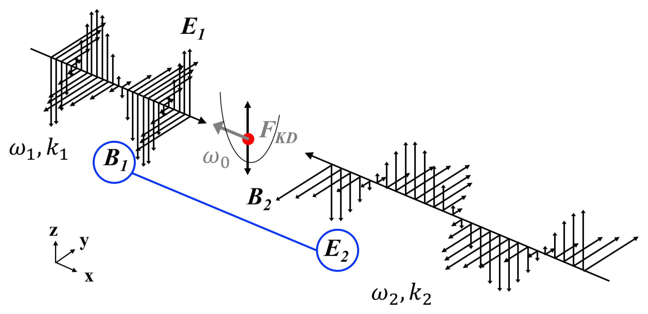
2. Kapitza–Dirac Force on Harmonic Oscillators

Let us consider the setup in Figure 1. Two counter-propagating laser fields propagate along the x-axis, and the electric fields are linearly polarized along the z-axis:

$$\begin{array}{cc}\hfill {\mathbf{E}}_1=& A_1{\omega }_{1}cos(k_{1}x-{\omega }_{1}t){\widehat{ϵ}}_z,\hfill \\ \hfill {\mathbf{E}}_2=& -A_2{\omega }_{2}cos(k_{2}x+{\omega }_{2}t){\widehat{ϵ}}_z,\hfill \end{array}$$

(1)

where ${\widehat{ϵ}}_z$ is the unit vector along the z-axis, $k_{1,2}={\omega }_{1,2}/c$ are the wave numbers, and $A_{1,2}$ are amplitudes of the corresponding vector potentials ${\mathbf{A}}_1=A_{1}sin(k_{1}x-{\omega }_{1}t){\widehat{ϵ}}_z$ and ${\mathbf{A}}_2=A_{2}sin(k_{2}x+{\omega }_{2}t){\widehat{ϵ}}_z$. The electric and magnetic components of the combined laser field are:

$$\begin{array}{c}\hfill E_z=A_1{\omega }_{1}cos(k_{1}x-{\omega }_{1}t)-A_2{\omega }_{2}cos(k_{2}x+{\omega }_{2}t),\\ \hfill B_y=-A_1{k}_{1}cos(k_{1}x-{\omega }_{1}t)-A_2{k}_{2}cos(k_{2}x+{\omega }_{2}t).\end{array}$$

(2)

Assuming that the particle is free in the direction of the electric field (i.e., the z-axis in Figure 1), the cross terms between the electric and magnetic components can give rise to a spatially modulated force in the direction of wave propagation (i.e., the x-axis in Figure 1). Herein, we term this force the Kapitza–Dirac (KD) force. The KD force can be derived using the following equations of motion:

$$\left\{\begin{array}{c}{\displaystyle m\frac{d{v}_z}{dt}=q{E}_z}\hfill \\ {\displaystyle F_x^{\left(\mathrm{KD}\right)}=q{v}_z{B}_y}\hfill \end{array}\right.,$$

(3)

where m and q are mass and charge of the particle. Now, there are two scenarios: (1) If frequencies of the two laser fields are identical (${\omega }_1={\omega }_2$), the KD force will be constant in time, which is also known as the pondermotive force [32], whereas (2) if the laser frequencies are different (${\omega }_1\ne {\omega }_2$), the KD force will oscillate in time with the sum and difference frequencies, ${\omega }_1+{\omega }_2$ and ${\omega }_1-{\omega }_2$. If the charge particle is confined by a harmonic potential $U\left(x\right)=m{\omega }_0^2{x}^2/2$ with a resonant frequency ${\omega }_0=({\omega }_1-{\omega }_2)/2$, the KD force that can resonantly drive the harmonic oscillator will be (see derivation in Appendix A):

$$F_{\mathrm{KD}}=\frac{q^2{A}_1{A}_2}{m}\left(\frac{k_1+k_2}{2}\right)sin\left((k_1+k_2)x\right)cos\left(({\omega }_1-{\omega }_2)t\right).$$

(4)

Accordingly, the corresponding time-varying KD potential is:

$$U_{\mathrm{KD}}=\frac{q^2{A}_1{A}_2}{2m}cos\left((k_1+k_2)x\right)cos\left(({\omega }_1-{\omega }_2)t\right).$$

(5)

We note that at any given time $t=t_0$, a trapping site in the KD potential $U_{\mathrm{KD}}(x,t_0)$ (i.e., a minimum in the potential) will turn into an unstable point after a quarter of the natural period $T_0/4=\pi /|{\omega }_1-{\omega }_2|$, where $T_0=2\pi /{\omega }_0$, since the potential polarity is reversed:

$$U_{\mathrm{KD}}(x,t_0+T_0/4)=-U_{\mathrm{KD}}(x,t_0).$$

(6)

This feature will later be used to coherently split the ground-state wavepacket of a quantum oscillator.

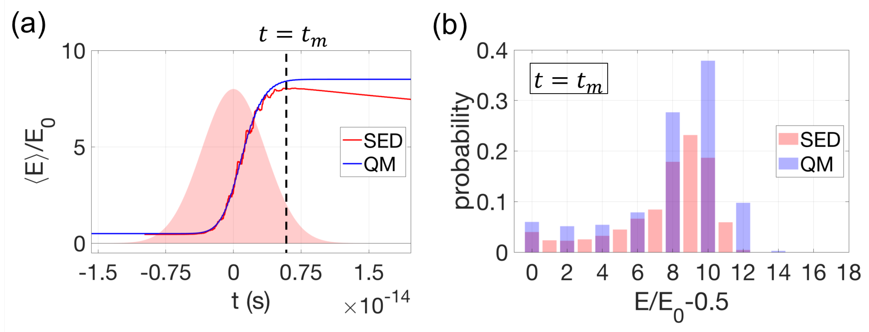
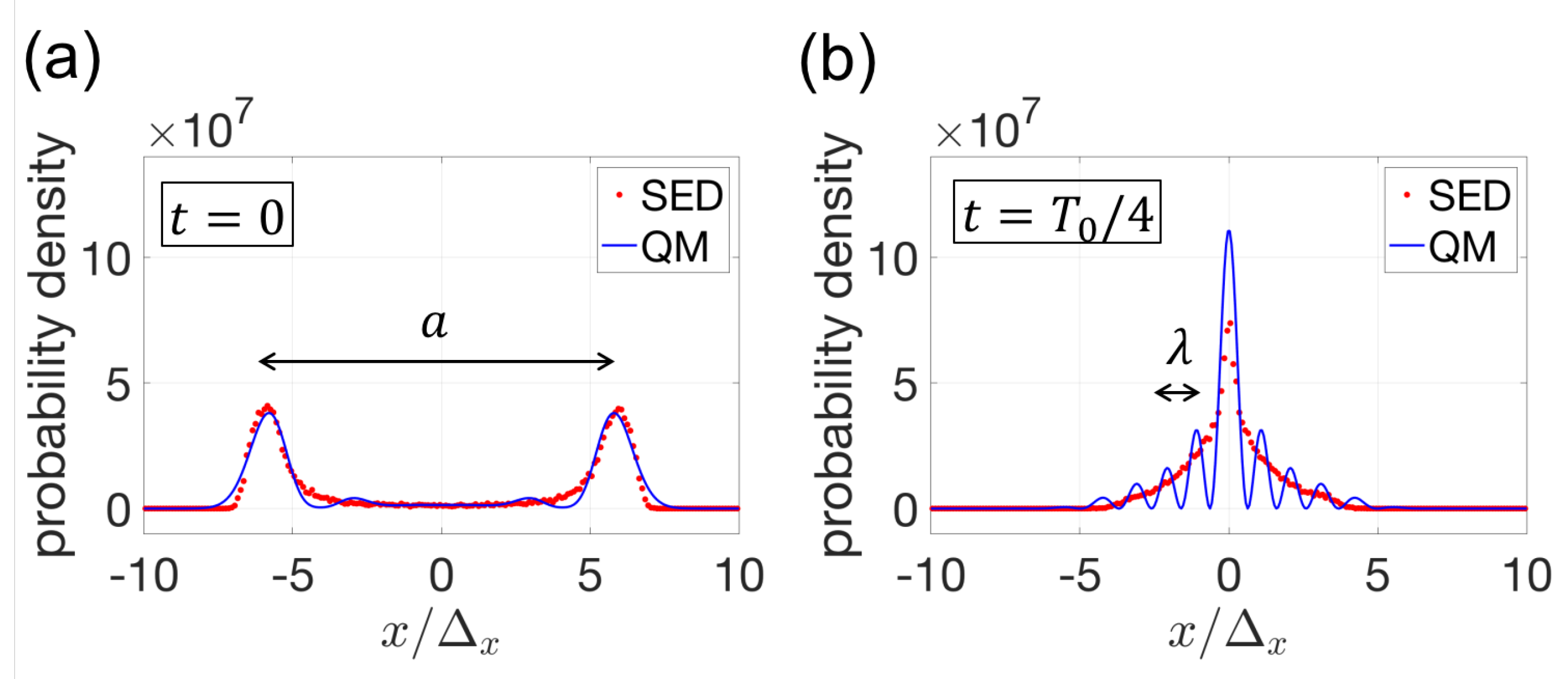
3. Generation of Squeezed Schrödinger Cat States

The KD effect for quantum harmonic oscillators can be modeled by adding the KD potential in Equation (5) to the unperturbed oscillator Hamiltonian. We replace the continuous-wave laser fields in Equation (1) with pulsed fields:

$$\begin{array}{cc}\hfill {\mathbf{E}}_1(x,t)& =A_1{\omega }_{1}cos(k_{1}x-{\omega }_{1}t)e^{-{(t/\tau )}^2}{\widehat{ϵ}}_z,\hfill \\ \hfill {\mathbf{E}}_2(x,t)& =-A_2{\omega }_{2}cos(k_{2}x+{\omega }_{2}t)e^{-{(t/\tau )}^2}{\widehat{ϵ}}_z,\hfill \end{array}$$

(7)

where $\tau$ is the pulse duration, in order to avoid indefinite sequential excitation of the oscillator’s ladder levels. Given the appropriate pulse amplitudes and durations, the final population distribution can have a peaked structure. The quantum Hamiltonian is thus:

$$\widehat{H}=\frac{m{\omega }_0}{2}{\widehat{x}}^2+\frac{{\widehat{p}}^2}{2m}+U_{KD}(\widehat{x},t)e^{-2{(t/\tau )}^2}.$$

(8)

The difference frequency of the laser fields is twice the oscillator’s resonant frequency ${\omega }_1-{\omega }_2=2{\omega }_0$, so the ground-state oscillator will be parametrically excited to the even-symmetry states $|n=2k\rangle$, which is a prerequisite for cat state generation because a cat state has an even symmetry. We obtained the QM result by numerically solving the Schödinger equation as in Reference [18]. The oscillator’s parameters are $m=9.11\times {10}^{-35}$ (kg), $q=1.60\times {10}^{-19}$ (C), and ${\omega }_0={10}^{16}$ (rad/s). The laser parameters are chosen to be ${\omega }_1=2.3{\omega }_0$, ${\omega }_2=0.3{\omega }_0$, $\tau =5\times {10}^{-15}$ (s), and $A_1=A_2=4.5\times {10}^{-8}$ (V·s/m). The mass is chosen at this unusual value in order to make the computational time for SED simulation more manageable [8]. In Figure 2b, the probability trajectory of the excited state is shown. Upon excitation, the ground-state wavepacket is coherently split into two wavepackets, so the oscillator is in a superposition of two macroscopically distinct states. The two wavepackets oscillate back and forth in the harmonic potential. As they recombine, interference fringes emerge in the probability distribution due to the quantum coherence between the two wavepackets. The quantum coherence is readily illustrated by the fringe structure in the oscillator’s Wigner function, as shown in Figure 2a. We note that one of the two quadrature uncertainties of each wavepacket, ${\sigma }_x\equiv \sqrt{\langle x^2\rangle -{\langle x\rangle }^2}$ (or ${\sigma }_p\equiv \sqrt{\langle p^2\rangle -{\langle p\rangle }^2}$), is smaller than the ground state uncertainty ${\Delta }_x=\sqrt{\hslash /2m{\omega }_0}$ (or ${\Delta }_p=\sqrt{\hslash m{\omega }_0/2}$), while their product remains the same, ${\sigma }_x{\sigma }_p=\hslash /2$, at all times (see Figure 2a). This implies that the state generated by the laser excitation is a squeezed Schrödinger cat state (that is, a superposition of two displaced squeezed states with opposite phases) [29,30].

For SED oscillators, we first prepared the classical ensemble in a ground state with the x and p probability distributions identical to those of a quantum oscillator (see details in Reference [8]). Under excitation of the same laser pulses, the equation of motion for the SED harmonic oscillator is:

$$m\frac{d^{2}x}{d{t}^2}=-m{\omega }_0^{2}x-m\mathrm{\Gamma }{\omega }_0^2\frac{dx}{dt}+q{E}_{vac}^{\left(x\right)}(x,t)+F_{\mathrm{KD}}(x,t)e^{-2{(t/\tau )}^2},$$

(9)

where ${\displaystyle \mathrm{\Gamma }\equiv \frac{2q^2}{3m{c}^3}\frac{1}{4\pi {ϵ}_0}}$ is the radiation damping coefficient. The zero-point field $E_{vac}^{\left(x\right)}(x,t)$ is configured according to Reference [8]. Apart from the damping term $m\mathrm{\Gamma }{\omega }_0^{2}dx/dt$ and the coupling to the zero-point field $E_{vac}^{\left(x\right)}(x,t)$, Equation (9) is formally equivalent to a quantum Heisenberg equation derived from the Hamiltonian in Equation (8). This suggests that the excitation dynamics in SED should be identical to QM, assuming (1) the pulse duration $\tau$ is much shorter than the damping time ${\tau }_d=2/\mathrm{\Gamma }{\omega }_0^2$, and (2) the KD force is much stronger than the fluctuating force from the zero-point field [8]:

$$\frac{q^2{A}_1{A}_2}{m}\left(\frac{k_1+k_2}{2}\right)\gg \frac{q}{2\pi }\sqrt{\frac{\hslash \mathrm{\Gamma }{\omega }_0^5}{{ϵ}_0{c}^3}}.$$

(10)

In our simulation, these two conditions are satisfied, and the excitation dynamics in SED and QM are the same as shown in Figure 3a, where the time evolutions of the expectation value of the QM energy and the ensemble average of the SED energy are compared. The two energy trajectories stay overlapped through most of the pulse and only deviate at the end of the excitation. Furthermore, the SED and QM energy distributions have similar shapes (see Figure 3b), despite the fact that the QM distribution is discrete and the SED distribution is continuous.

The probability trajectory of the SED oscillator ensemble along with its phase space distribution are shown in Figure 2c,d. The ensemble particle number is $N_p=3\times {10}^4$. The parametric interaction between the SED oscillator and the laser fields were simulated using the same method as in Reference [18]. Like the QM oscillator, upon excitation, the ground-state SED probability distribution also splits into two sub-ensembles that follow two distinct sinusoidal trajectories. The initial phase spectrum of the zero-point field, which is random and considered as the “hidden variable”, determines which trajectory a particle will follow in each trial. A detailed comparison between SED and QM probability distributions is given in Figure 4 for two time points: (1) When the two QM wavepackets are separated and (2) when they recombine. Although there are some overall similarities between the SED and QM distributions, there are no interference fringes in the SED probability distribution.

4. Discussion and Conclusions

While the zero-point electromagnetic field only introduces small radiative corrections to nonrelativistic QM, such as Lamb shifts, it drastically changes the particle dynamics in classical mechanics and leads to the reproduction of QM effects in some classical systems [6,7,8,9,11,12,13,18]. Our work aimed to investigate to what extent such a classical theory can reproduce QM features by comparing results obtained from SED, Equation (9), with those obtained from the QM Hamiltonian, Equation (8). The qualitative difference between the probability distributions of QM and SED in Figure 2 and Figure 4b establishes that SED in its traditional form does not support physical effects that involve quantum coherence [4,5]. The squeezed Schrödinger cat state used in this work is an analogy of the electron double-slit experiment [19]. The peak-to-peak separation a between the two wavepackets in Figure 4a determines the fringe periodicity $\lambda$ in Figure 4b through the relation $\lambda =2\pi \hslash /m{\omega }_{0}a$, which mimics the double-slit diffraction formula. Our analysis provides evidence that coherence-like behavior is absent in SED, and thus, we predict that SED electron double-slit diffraction, if ever calculated, will not show fringes.

On the other hand, our result helps to establish the validity range of SED. We note that the partial agreement between the SED and QM results stems from the formal resemblance between the SED equation of motion and the QM Heisenberg equation, assuming that the laser excitation pulses satisfy certain criteria. While x and p are independent dynamic variables in SED, the canonical commutation relation $[\widehat{x},\widehat{p}]=i\hslash$ makes them a Fourier pair in QM. This difference makes the distinction between QM and SED in terms of quantum coherence. Therefore, SED may be seen as the decoherence limit of QM [33]. Although the zero-point field bestows a special phase relation between x and p of a SED harmonic oscillator, which leads to the quantum ground-state distributions [7,8], the phase relation serves only as initial conditions and does not affect the dynamical evolution of x and p during laser excitation. Therefore, we speculate that any mechanism or theoretical operation that restores (or deteriorates) the Fourier relation between x and p for SED (or QM) will make the proper decoherence theory that bridges the gap between SED and QM.

References

1. De la Pe na, L.; Cetto, A.M. The Quantum Dice: An Introduction to Stochastic Electrodynamics; Springer: New York, NY, USA, 1996. [Google Scholar]
2. De la Pe na, L.; Cetto, A.M.; Valdes-Hernandez, A. Emerging Quantum: The Physics Behind Quantum Mechanics; Springer: New York, NY, USA, 2015. [Google Scholar]
3. Cavalleri, G.; Barbero, F.; Bertazzi, G.; Cesaroni, E.; Tonni, E.; Bosi, L.; Spavieri, G.; Gillies, G. Aquantitative assessment of stochastic electrodynamics with spin (SEDS): Physical principles and novel applications. Front. Phys. China 2010, 5, 107. [Google Scholar] [CrossRef]
4. Milonni, P.W. The Quantum Vacuum: An Introduction to Quantum Electrodynamics; Academic Press: Cambridge, MA, USA, 1994. [Google Scholar]
5. Boyer, T.H. Random electrodynamics: The theory of classical electrodynamics with classical electromagnetic zero-point radiation. Phys. Rev. D 1975, 11, 790. [Google Scholar] [CrossRef]
6. Boyer, T.H. Retarded van der Waals Forces at All Distances Derived from Classical Electrodynamics with Classical Electromagnetic Zero-Point Radiation. Phys. Rev. A 1973, 7, 1832. [Google Scholar] [CrossRef]
7. Boyer, T.H. General connection between random electrodynamics and quantum electrodynamics for free electromagnetic fields and for dipole oscillator systems. Phys. Rev. D 1975, 11, 809–830. [Google Scholar] [CrossRef]
8. Huang, W.C.; Batelaan, H.J. Dynamics Underlying the Gaussian Distribution of the Classical Harmonic Oscillator in Zero-Point Radiation. Comput. Methods Phys. 2013, 2013, 308538. [Google Scholar] [CrossRef]
9. Boyer, T.H. Diamagnetism of a free particle in classical electron theory with classical electromagnetic zero-point radiation. Phys. Rev. A 1980, 21, 66–72. [Google Scholar] [CrossRef]
10. Boyer, T.H. Understanding the Planck blackbody spectrum and Landau diamagnetism within classical electromagnetism. Eur. J. Phys. 2016, 37, 065102. [Google Scholar] [CrossRef]
11. Boyer, T.H. Derivation of the blackbody radiation spectrum from the equivalence principle in classical physics with classical electromagnetic zero-point radiation. Phys. Rev. D 1984, 29, 1096. [Google Scholar] [CrossRef]
12. Boyer, T.H. Scaling, scattering, and blackbody radiation in classical physics. Eur. J. Phys. 2017, 38, 045101. [Google Scholar] [CrossRef]
13. Blanco, R.; Franca, H.M.; Santos, E. Classical interpretation of the Debye law for the specific heat of solids. Phys. Rev. A 1991, 43, 693. [Google Scholar] [CrossRef] [PubMed]
14. Puthoff, H.E. Ground state of hydrogen as a zero-point-fluctuation-determined state. Phys. Rev. D 1987, 35, 3266–3269. [Google Scholar] [CrossRef]
15. Cole, D.C.; Zou, Y. Quantum mechanical ground state of hydrogen obtained from classical electrodynamics. Phys. Lett. A 2003, 317, 14–20. [Google Scholar] [CrossRef]
16. Nieuwenhuizen, T.M.; Liska, M.T.P. Simulation of the hydrogen ground state in stochastic electrodynamics. Phys. Scr. 2015, T165, 014006. [Google Scholar] [CrossRef]
17. Nieuwenhuizen, T.M. On the stability of classical orbits of the hydrogen ground state in Stochastic Electrodynamics. Entropy 2016, 18, 135. [Google Scholar] [CrossRef]
18. Huang, W.C.; Batelaan, H. Discrete excitation spectrum of a classical harmonic oscillator in zero-point radiation. Found. Phys. 2015, 45, 333–353. [Google Scholar] [CrossRef]
19. Bach, R.; Pope, D.; Liou, S.-H.; Batelaan, H. Controlled double-slit electron diffraction. New J. Phys. 2013, 15, 033018. [Google Scholar] [CrossRef]
20. Avenda no, J.; de la Pe na, L. Dynamic electron control using light and nanostructure. Phys. Rev. E 2004, 72, 066605. [Google Scholar]
21. Kracklauer, A.F. An Intutive Paragidm for Quantum Mechanics. Phys. Essays 1992, 5, 226. [Google Scholar] [CrossRef]
22. Wolchover, N. Famous Experiment Dooms Alternative to Quantum Weirdness. Quanta Magazine, 11 October 2018. [Google Scholar]
23. Couder, Y.; Fort, E. Single-particle diffraction and interference at a macroscopic scale. Phys. Rev. Lett. 2006, 97, 154101. [Google Scholar] [CrossRef]
24. Andersen, A.; Madsen, J.; Reichelt, C.; Ahl, S.R.; Lautrup, B.; Ellegaard, C.; Levinsen, M.T.; Bohr, T. Double-slit experiment with single wave-driven particles and its relation to quantum mechanics. Phys. Rev. E 2015, 92, 013006. [Google Scholar] [CrossRef]
25. Bohr, T.; Andersen, A.; Lautrup, B. Recent Advances in Fluid Dynamics with Environmental Applications; Springer: New York, NY, USA, 2016; pp. 335–349. [Google Scholar]
26. Batelaan, H.; Jones, E.; Huang, W.C.; Bach, R. Momentum exchange in the electron double-slit experiment. J. Phys. Conf. Ser. 2016, 701, 012007. [Google Scholar] [CrossRef]
27. Pucci, G.; Harris, D.M.; Faria, L.M.; Bush, J.W.M. Walking droplets interacting with single and double slits. J. Fluid Mech. 2018, 835, 1136–1156. [Google Scholar] [CrossRef]
28. Kienzler, D.; Flühmann, C.; Negnevitsky, V.; Lo, H.-Y.; Marinelli, M.; Nadlinger, D.; Home, J.P. Observation of quantum interference between separated mechanical oscillator wave packets. Phys. Rev. Lett. 2016, 116, 140402. [Google Scholar] [CrossRef]
29. Etesse, J.; Bouillard, M.; Kanseri, B.; Tualle-Brouri, R. Experimental generation of squeezed cat states with an operation allowing iterative growth. Phys. Rev. Lett. 2015, 114, 193602. [Google Scholar] [CrossRef]
30. Huang, K.; le Jeannic, H.; Ruaudel, J.; Verma, V.B.; Shaw, M.D.; Marsili, F.; Nam, S.W.; Wu, E.; Zeng, H.; Jeong, Y.-C.; et al. Optical synthesis of large-amplitude squeezed coherent-state superpositions with minimal resources. J. Phys. Rev. Lett. 2015, 115, 023602. [Google Scholar] [CrossRef]
31. Tonomura, A.; Endo, J.; Matsuda, T.; Kawasaki, T.; Ezawa, H. Demonstration of single-electron buildup of an interference pattern. Am. J. Phys. 1989, 57, 117. [Google Scholar] [CrossRef]
32. Batelaan, H. Colloquium: Illuminating the Kapitza-Dirac effect with electron matter optics. Rev. Mod. Phys. 2007, 79, 929–941. [Google Scholar] [CrossRef]
33. Sonnentag, P.; Hasselbach, F. Measurement of decoherence of electron waves and visualization of the quantum-classical transition. Phys. Rev. Lett. 2007, 98, 200402. [Google Scholar] [CrossRef]
Figure 1. Two counter-propagating laser fields with frequencies ω 1 and ω 2 collaboratively drive the harmonic oscillator with a spatially modulated Kapitza–Dirac force in the direction of wave propagation. The force has a modulation periodicity of 2 π c / ( ω 1 + ω 2 ) , and it oscillates at the difference frequency ω 1 ω 2 . A particle subject to the perturbation of the classical zero-point electromagnetic field can get pushed to either directions.
Atoms 07 00042 g001
Figure 2. Time evolution of quantum mechanics (QM) and stochastic electrodynamics (SED) probability distributions after laser excitation. (a) The Wigner function of the QM oscillator is plotted after the laser excitation. Positive values are color-coded in red, and negative values are in blue. Quantum coherence between the two well-separated squeezed states is manifested by the fringe structure in the center. The Wigner function rotates counter-clockwise at the oscillator’s resonant frequency ω 0 = 10 16 (rad/s). At the moment when the distribution is depicted, the position quadrature uncertainty σ x of the squeezed state is smaller than that of the ground state Δ x = / 2 m ω 0 . Meanwhile, the quadrature uncertainty product satisfies the Heisenberg relation σ x σ p = / 2 at all times. (b) The two wavepackets oscillate back and forth in the harmonic potential, giving rise to a double sinusoidal trajectory of the QM probability distribution. An interference pattern appears when the two wavepackets merge. (c) The phase space distribution of the SED oscillator shows two well-separated sub-ensembles. Each sub-ensemble has a squeezed structure that mimics the QM squeezed state shown in (a). (d) As the SED phase space distribution rotates counter-clockwise, the probability distribution bundles into two “macroscopic” trajectories. In each trial of the SED simulation, there is no knowledge which macroscopic trajectory a particle will follow unless the initial phase of the background zero-point field is known. No interference-like patterns are found in the SED probability distribution when the two macroscopic trajectories of distributions cross.
Atoms 07 00042 g002
Figure 3. The QM and SED energy distributions after laser excitation. (a) The ensemble average of the SED oscillator energy (red line) is compared with the expectation value of the QM oscillator energy (blue line) during the course of laser excitation. The shaded area (red) represents the excitation laser pulse e ( t / τ ) 2 . The pulse duration is τ = 5 × 10 15 (s), which is much smaller than the SED oscillator damping time τ d 3.2 × 10 13 (s). Therefore, damping has no significant effect on the oscillator’s dynamics during the excitation process. (b) Energy distributions of QM and SED oscillators are compared at t = t m when the SED energy reaches its maximum and the radiation damping starts to dominate. The QM energy distribution (blue bar) is discrete and occupies only even energy levels E 2 k = E 0 ( 2 k + 1 / 2 ) , where E 0 = ω 0 . The SED energy distribution (red bar) is continuous but has a similar width and average value as the QM distribution. This indicates that the excitation process is identical for QM and SED oscillators.
Atoms 07 00042 g003
Figure 4. Comparison between the QM and SED probability distributions at t = 0 and t = T 0 / 4 in Figure 2. (a) The agreement between QM and SED probability distributions is good when the two macroscopically distinct QM wavepackets are well-separated by a peak-to-peak distance a beyond the ground state width Δ x , a Δ x . (b) After a quarter of the natural period T 0 / 4 , the two QM wavepackets recombine in the harmonic potential. Interference fringes appear in the QM distribution (blue line) but not in the SED distribution (red dots). The fringe periodicity λ is determined by the wavepacket separation a in (a) through the relation λ = 2 π / m ω 0 a , which resembles the well-known double-slit diffraction formula. The SED probability distribution captures the outline of the QM distribution as if the quantum coherence between the two QM wavepackets is lost.
Atoms 07 00042 g004