Abstract
The accuracy of approximate automodel solutions for the Green’s function of the Biberman-Holstein equation for the Stark broadening of spectral lines is analyzed using the distributed computing. The high accuracy of automodel solutions in a wide range of parameters of the problem is shown.
1. Introduction
The Stark broadening of spectral lines is known to produce the long-tailed spectral line shapes of atom and ion radiation in plasmas (see, e.g., [1,2,3,4,5,6,7,8]). In the broad range of conditions in plasmas and gases, where the complete redistribution (CRD) in photon frequency within the resonance line shape is applicable, the radiative transfer is described by the Biberman-Holstein equation for the density of excited atoms [9,10] and characterized by the infinite mean-squared displacement of the initial perturbation [11] and, respectively, by the irreducibility of the integral equation, in space variables, to a differential one. This makes the respective radiative transfer a nonlocal (superdiffusive) one [12,13] (for the deviation from the CRD and the limits of its applicability see, e.g., [14,15,16]).
The latter makes the numerical simulation of radiative transfer in resonance spectral lines a formidable task. The simple models based on the domination of the long-free-path flights of the photons were suggested [17] and developed for the quasi-steady-state transport problem, now known as the escape probability methods (see [18,19,20]).
For the time-dependent superdiffusive transport, recently, a wide class of non-steady-state superdiffusive transport on a uniform background with a power-law decay, at large distances, of the step-length probability distribution function (PDF) was shown [21] to possess an approximate automodel solution. The solution for the Green’s function was constructed using the scaling laws for the propagation front (i.e., time dependence of the relevant-to-superdiffusion average displacement of the carrier) and asymptotic solutions far beyond and far ahead the propagation front. These scaling laws were shown to be determined essentially by the long free-path carriers (Lévy flights [22,23,24,25,26]). The validity of the suggested automodel solution was proved by its comparison with numerical solutions in the one-dimensional (1D) case of the transport equation with a simple long-tailed PDF with various power-law exponents and in the case of the Biberman-Holstein equation of the 3D resonance radiative transfer for various (Doppler, Lorentz, Voigt, and Holtsmark) spectral line shapes. The analysis of the limits of applicability of the automodel solution in the above-mentioned cases was continued in [27]. The full-scale numerical analysis of the limits of applicability was done in [28], using the massive computations of the exact solution of the transport equation with a simple long-tailed PDF with various power-law exponents. The comparison of these results with automodel solutions has shown high accuracy of automodel solutions in a wide range of space-time variables and enabled us to identify the limits of applicability of the automodel solutions.
It is important to note that the success of automodel solutions [21] for a wide class of non-stationary superdiffusive transport was achieved due to identification of the scaling laws in the case of radiative transfer in the Biberman-Holstein model in [11,12,13,17,21,29,30,31,32,33].
The Stark broadening of spectral lines is, itself, a highly complicated problem (see, e.g., [34] for the efforts, based on the quantum kinetic theory approach to the line broadening, to eliminate the remaining discrepancy of theory and experiment). The allowance for radiative transfer effects under conditions of the Stark broadening of spectral lines substantially complicates the diagnostics of the medium’s parameters (see, e.g., the case of steady-state transport in inhomogeneous plasmas [35]). In light of these issues, the automodel solutions of the time-dependent Green’s function of the radiative transfer equation in homogeneous media, considered in the present paper, may serve as reliable benchmarks for radiative transfer models in various applications.
Here we extend the approach [28] to the case of the Green’s function of the 3D Biberman-Holstein equation for the Voigt spectral line shape, assuming the contribution of the impact Stark broadening to the Lorentz component of the Voigt line shape (Section 2.2.2). Additionally, the results for the case of Holtsmark line shape are presented (Section 2.2.3). The main equations are given in Section 2.1, and conclusions are made in Section 3.
2. Results
2.1. Main Equations
2.1.1. Biberman–Holstein Equation
The Biberman–Holstein equation [9,10] for radiative transfer in a uniform medium of two-level atoms/ions has been obtained from the system of equations for spatial density of excited atoms, F(r, t), and spectral intensity of resonance radiation. This system is reduced to a single equation for F(r, t), which appears to be an integral equation, non-reducible to a differential diffusion-type equation:
where τ is the lifetime of the excited atomic state with respect to spontaneous radiative decay; σ is the rate of the collisional quenching of excitation; q is the source of excited atoms, different from populating by the absorption of resonant photons (e.g., collisional excitation). The kernel G is determined by the (normalized) emission spectral line shape εv and the absorption coefficient kv. In homogeneous media, G depends on the distance between the points of emission and absorption of the photon:
The analytical solution of Equation (1) with a point instant source, q(r, t) = δ(r)δ(t), i.e., the Green’s function, was obtained in [11] with the help of the Fourier transform:
where:
The homogeneity of the medium implies that τ and σ are constants. The latter makes the role of quenching easily accounted for by the time exponent exp(–σt), so in what follows we omit the account of this process, i.e., in fact, for convenience we take σ = 0. Hereafter we use the dimensionless time, assuming the normalization by τ.
Equation (3) for r ≠ 0 may be transformed to take the following form:
Let us consider two cases where the Stark broadening plays a dominant role in the resonance radiative transfer in the Biberman–Holstein model, namely, the case of the Voigt spectral line shape, assuming the contribution of the impact Stark broadening to the Lorentz component of the Voigt spectral line shape (Section 2.1.2), and the case of the static Stark broadening in the Holtsmark model (Section 2.1.3).
2.1.2. Exact Solution for Voigt Spectral Line Shape
The line shape εν is taken in the form [36]:
where:
Here is the full width at half maximum (FWHM) of the Doppler line shape, and is the FWHM of the Lorentz line shape. The coefficient is determined by the normalization condition, . For the Stark broadening of the spectral line shape one may use the well-known formulae for the impact broadening, e.g., in the monographs [1,2], and learn the progress in the recent surveys [37,38].
The respective absorption coefficient kν(a) has the form:
where n0 is the density of absorbing atoms, λ, the wavelength of a photon, , statistical weight of the i-th level. Using Equation (3.466.1) in [39], may be expressed in the form:
where erf(x) is the error function:
Let us turn in Equation (5) to dimensionless variables ρ = k0r and P = p/k0, and use Equations (6) and (10) for εν and kν. This gives:
2.1.3. Exact Solution for Holtsmark Spectral Line Shape
For Holtsmark spectral line shape the functions εν and kν, which enter the function J(p), for linear Stark effect may be expressed in the form (cf. [3]):
where N is the density of the perturbing particles, and is the Holtsmark function:
Turning in Equation (5) to dimensionless variables ρ = k0r and P = p/k0, and using Equations (17) and (18) for εν and kν, we obtain:
2.2. Approximate Automodel Solution and Verification for Accuracy
2.2.1. General Equations
The approximate automodel solution [21] has the form:
where G is the kernel of the Biberman-Holstein equation, g is an unknown function with the following asymptotics:
For the propagation front, , we used in [21,28] the function which appears to be close to the time dependence of the mean displacement:
Alternatively, one may use another function which appears to work better in the case of spectral line shape which is a convolution of two essentially different line shapes (e.g., for Voigt line shape):
where:
The relation between g and the exact solution of Equation (1), fexact, is described by the following equation:
where G−1 is the function reciprocal to the G function, ρ ≡ k0|r – r0|, k0 is the absorption coefficient for photons at the frequency, corresponding to the line shape center:
where the functions t(ρ, s) and ρ(t, s) are determined by the relation:
To prove the automodel solution one has to show weak dependence (independence) of QG1 and QG2 functions on, respectively, the space coordinate and time. The results of the validation of the automodel solution and the reconstruction of function g from comparison of function (21) with computations of the Green’s function for the Voigt and Holtsmark line shapes are given in what follows.
2.2.2. Automodel Solution for the Voigt Spectral Line Shape
The convolution of two line shapes with essentially different wings, an exponential one, for the Doppler case, and a power-law one, for the Lorentz case, makes the superdiffusive radiative transfer very sensitive to the contribution of the power-law wings of spectral line to the resulting long-tailed PDF. This is illustrated with the Figure 1 where the dependence of the exponent in the exact solution (Equation (15)) is shown. It is seen that even a small fraction of the Lorentz line shape in the Voigt line shape produces strong effects at large distances (for small values of p, respectively).

Figure 1.
Dependence of the expression (1 – J(P, a)), where J is given by Equation (16) on the variable P for various values of a which is the Lorentz-to-Doppler width ratio in the Voigt spectral line shape.
We illustrate the results of accuracy analysis with three figures. First, the functions QG2(s,t) (Equation (29)) are shown for different values of t in the range from tmin = 30 to tmax = 106. Further, the normalized functions QG2(s,t)/{QG2}av(s), where subscript av denotes averaging over time from tmin = 30 to tmax = 108, and the relative errors of the automodel solution fauto(ρ,t)/fexact(ρ,t) are shown for the same range of time.
The results of analysis for various values of the Voigt parameter a are shown in Figure 2.
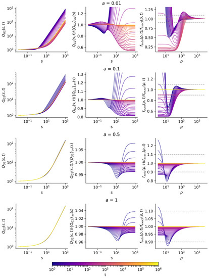
Figure 2.
The result of accuracy analysis of automodel solution for various values of the Voigt parameter and the propagation front ρ = ρfr taken in the form of Equation (24), for different values of t in the range from tmin = 30 to tmax = 106: (left) Functions QG2(s,t) (29); (center) normalized functions QG2(s,t)/{QG2}av(s), where subscript av denotes averaging over time from tmin = 30 to tmax = 108; and (right) relative errors of the automodel solution fauto(ρ,t)/fexact(ρ,t).
For applications it is of interest to determine the limits of applicability of the automodel solutions with a certain accuracy. To this end, in Figure 3 we show the level lines of the relative deviation of the automodel solution from the exact one, for the results from Figure 2.
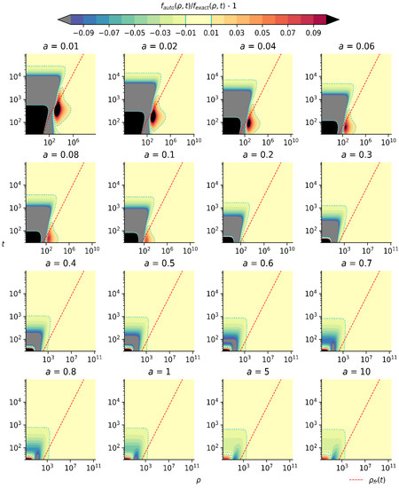
Figure 3.
The level lines of the relative deviation of the automodel solution from the exact one, for the results from Figure 2.
It is seen that for the Lorentz-dominated line shapes, i.e., moderate and large values of the Voigt parameter a, the accuracy of automodel solution is high in almost the entire space of variables {ρ, t}, quite similar to the case [21,28] of the superdiffusive transport for a 1D model PDF with the power-law wings. However, for a small a, the accuracy dramatically falls down in the essential part of the space of variables {ρ, t}. This failure stimulated searching for improving the accuracy by using the propagation front (Equation (25)). The respective results are shown in Figure 4 and Figure 5.
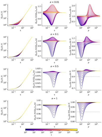
Figure 4.
The same as in Figure 2, but for the propagation front ρ = ρfr taken in the form of Equation (25).
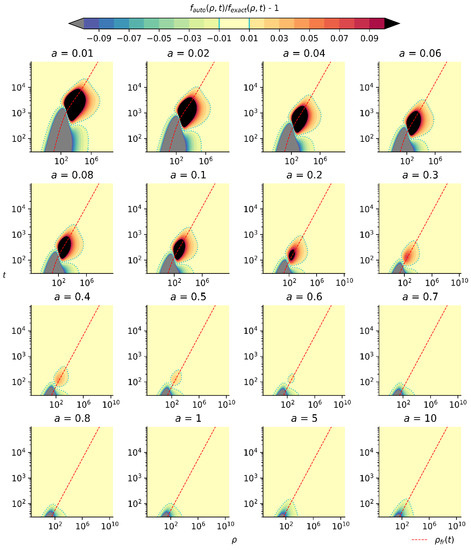
Figure 5.
The same as in Figure 3, but for the propagation front ρ = ρfr taken in the form of Equation (25).
Figure 3 and Figure 5 show that the automodel solution with the propagation front ρ = ρfr (Equation (25)) substantially improves the accuracy in the regions of the failure of the automodel solution with the propagation front (Equation (24)). This issue points to the possibility to further improve the accuracy by the variation of the definition of the propagation front and further verification of the accuracy of the respective automodel function via calculations of the exact solution in a limited part of the space of variables {ρ, t} (not in the entire space, only in the region around the propagation front).
2.2.3. Automodel Solution for the Holtsmark Spectral Line Shape
Here we append the results [21,27] of analyzing the automodel solution for the Holtsmark line shape with the results for the accuracy of automodel solution. Figure 6 shows the behavior of the automodel function QG2 (29) and the relative deviation of the automodel solution from the exact one in the range from tmin = 40 to tmax = 103, with the time step equal to 20, for 40 ≤ t ≤ 500, and 50, for 500 < t ≤ 1000.


Figure 6.
The result of accuracy analysis of automodel solution for the propagation front ρ = ρfr taken in the form of Equation (24), for different values of t in the range from tmin = 40 to tmax = 103 with the time step equal to 20, if 40 ≤ t ≤ 500. and 50, if 500 < t ≤ 1000: (a) functions QG2(s,t) (29); (b) normalized functions QG2(s,t)/{QG2}*(s,t), where {QG2}*(s,t) is equal to QG2(s,t = 160), for small s, and QG2(s,t = 103), for large s; (c) relative error of the automodel solution fauto(ρ,t)/fexact(ρ,t); and (d) the same in the 3D view.
The results show that, similarly to the 1D transport for a model step-length PDF with power-law wings [21,28], the accuracy of automodel solution is reasonably good for the propagation front (Equation (24)).
3. Discussion
The history of the research on the superdiffusive transport suggests that it is not possible to guess the “hidden” self-similarity from the general form of the transport equation, including the Biberman-Holstein equation, or from its analytical solutions in certain cases like the analytic solution [11] of the Biberman-Holstein equation. The approximate automodel (self-similar) solution [21] has been found thanks to:
- a hint from physics (namely, analysis of the kinetics of elementary excitation carriers); and
- interpolation of asymptotic solutions and solving an inverse problem which requires numerical simulations to verify the accuracy of the automodel solution and determine the limits of its applicability.
Obtaining automodel (self-similar) solutions in the entire space of independent variables requires mass numerical simulations, however, their total volume is significantly reduced due to the self-similarity of the solution.
The Stark broadening of spectral lines, including the contribution of the impact of Stark broadening to the Lorentz component of the Voigt line shape and the Holsmark broadening, produce the step-length probability distribution function (PDF) which makes the transport superdiffusive. The accuracy of approximate automodel solutions for the Green's function of the Biberman-Holstein equation for the Stark broadening of spectral lines is analyzed using the distributed computing. The high accuracy of automodel solutions in a wide range of parameters of the problem is shown. Massive computing experiments are conducted to verify automodel solutions. The Everest distributed computing platform and the cluster at the NRC ‘Kurchatov Institute’ are used. The results, obtained with distributed computing, verified the high accuracy of automodel solutions in a wide range of space-time variables and enabled us to identify the limits of applicability of automodel solutions.
The sensitivity of the automodel solution to the definition of the front propagation scaling is shown for the line shape with two quite different line broadening mechanisms, and the improvement of the accuracy of the automodel solution is achieved via generalization of the definition of the propagation front.
The present progress in describing the radiative transfer for infinite velocity of carriers, Equation (1), may be extended to the case of a finite velocity [40,41] (which includes the case of the resonance radiative transfer in astrophysics), where the exact solution and the asymptotics were also obtained [42].
4. Materials and Methods
Distributed computations have been done on the cluster at NRC “Kurchatov Institute” (http://ckp.nrcki.ru/) by means of the Everest (http://everest.distcomp.org/), a computing platform for publication, execution, and composition of applications running across distributed computing resources [43]. A generic Everest application, the so-called Parameter Sweep, (http://everest.distcomp.org/docs/ps) [44], was used to run a number of independent tasks at the cluster via a special Everest agent installed on the cluster. The calculation of exact and automodel solutions for a single value of parameter a in the Voight line shape (6) was an independent task. The values of a were taken in the range from 0.01 to 10, evenly spaced on a log scale, that yields 28 tasks. Since the two different expressions for the propagation front were considered (see Equations (24) and (25)) the total number of independent tasks was 56.
In order to obtain functions g(s), the exact solutions fexact(ρ,t) were calculated. The values of t were evenly spaced on a log scale in the range from tmin = 30 to tmax = 108. The values of s were also evenly spaced on a log scale. Depending on the value of a, the lower limit for s was set in the range from 0.00003 (small a) to 0.005 (large a) while the upper limit was set to 1000 for all values of a. The respective values of ρ are defined by the t and s numerical meshes, using Equation (30).
All analytic expressions of Equations (6)–(30) have been implemented in the form of a Python program, using the NumPy and SciPy, well-known scientific libraries (www.scipy.org).
In addition, direct comparison of the automodel (Equation (21)) and exact (Equation (15)) solutions of the transport Equation (1), the range of variables in the two-dimensional space, {time, space coordinate}, where the automodel solution is accurate within certain error bars around the exact solution was identified.
Author Contributions
All authors contributed equally to this work.
Funding
This research was partially funded by Russian Foundation for Basic Research (RFBR), grant numbers 18-07-01269 А, 17-07-00950 А, 18-07-01175 A.
Acknowledgments
This work has been carried out using computing resources of the federal collective usage center Complex for Simulation and Data Processing for Mega-science Facilities at NRC “Kurchatov Institute” (ministry subvention under agreement RFMEFI62117X0016), http://ckp.nrcki.ru/. The authors are grateful to A.V. Demura, V.S. Lisitsa, and E.A. Oks for helpful discussions, and A.P. Afanasiev for the support of collaboration between the NRC “Kurchatov Institute” and the Center for Distributed Computing (http://distcomp.ru) of the Institute for Information Transmission Problems (Kharkevich Institute) of Russian Academy of Science.
Conflicts of Interest
The authors declare no conflict of interest. The funders had no role in the design of the study; in the collection, analyses, or interpretation of data; in the writing of the manuscript, and in the decision to publish the results.
References
- Griem, H.R. Principles of Plasma Spectroscopy; Cambridge University Press: Cambridge, UK, 1997. [Google Scholar]
- Sobel’man, I.I. troduction to the Theory of Atomic Spectra; Pergamon Press: Oxford, UK, 1972. [Google Scholar]
- Kogan, V.I.; Lisitsa, V.S.; Sholin, G.V. Broadening of spectral lines in plasmas. In Reviews of Plasma Physics; Kadomtsev, B.B., Ed.; Consultants Bureau: New York, NY, USA, 1987; Volume 13, pp. 261–334. [Google Scholar]
- Lisitsa, V.S. New results on the Stark and Zeeman effects in the hydrogen atom. Sov. Phys. Usp. 1987, 30, 927–951. [Google Scholar] [CrossRef]
- Bureyeva, L.A.; Lisitsa, V.S. A Perturbed Atom; CRC Press: Boca Raton, FL, USA, 2000; ISBN 978-9058231383. [Google Scholar]
- Oks, E. Stark Broadening of Hydrogen and Hydrogenlike Spectral Lines in Plasmas: The Physical Insight; Alpha Science International: Oxford, UK, 2006; ISBN 978-1842652527. [Google Scholar]
- Oks, E. Diagnostics Of Laboratory And Astrophysical Plasmas Using Spectral Lines Of One-, Two-, and Three-Electron Systems; World Scientific: Hackensack, NJ, USA, 2017; ISBN 978-981-4699-07-5. [Google Scholar]
- Demura, A.V. Beyond the Linear Stark Effect: A Retrospective. Atoms 2018, 6, 33. [Google Scholar] [CrossRef]
- Biberman, L.M. On the diffusion theory of resonance radiation. Sov. Phys. JETP 1949, 19, 584–603. [Google Scholar]
- Holstein, T. Imprisonment of Resonance Radiation in Gases. Phys. Rev. 1947, 72, 1212–1233. [Google Scholar] [CrossRef]
- Veklenko, B.A. Green’s Function for the Resonance Radiation Diffusion Equation. Sov. Phys. JETP 1959, 9, 138–142. [Google Scholar]
- Biberman, L.M.; Vorob’ev, V.S.; Yakubov, I.T. Kinetics of Nonequilibrium Low Temperature Plasmas; Consultants Bureau: New York, NY, USA, 1987; ISBN 978-1-4684-1667-1. [Google Scholar]
- Abramov, V.A.; Kogan, V.I.; Lisitsa, V.S. Radiative transfer in plasmas. In Reviews of Plasma Physics; Leontovich, M.A., Kadomtsev, B.B., Eds.; Consultants Bureau: New York, NY, USA, 1987; Volume 12, p. 151. [Google Scholar]
- Starostin, A.N. Resonance radiative transfer. In Encyclopedia of Low Temperature Plasma. Introduction Volume; Fortov, V.E., Ed.; Nauka/Interperiodika: Moscow, Russia, 2000; Volume 1, p. 471. (In Russian) [Google Scholar]
- Sechin, A.Y.; Starostin, A.N.; Zemtsov, Y.K.; Chekhov, D.I.; Leonov, A.G. Resonance radiation transfer in dense dispersive media. J. Quant. Specrrosc. Radiat. Transf. 1997, 58, 887–903. [Google Scholar] [CrossRef]
- Bulyshev, A.E.; Demura, A.V.; Lisitsa, V.S.; Starostin, A.N.; Suvorov, A.E.; Yakunin, I.I. Redistribution function for resonance radiation in a hot dense plasma. Sov. Phys. JETP 1995, 81, 113–121. [Google Scholar]
- Biberman, L.M. Approximate method of describing the diffusion of resonance radiation. Doklady Akademii nauk SSSR Series Physics 1948, 49, 659. (In Russian) [Google Scholar]
- Napartovich, A.P. On the τeff method in the radiative transfer theory. High Temp. 1971, 9, 23–26. [Google Scholar]
- Kalkofen, W. Methods in Radiative Transfer; Kalkofen, W., Ed.; Cambridge University Press: Cambridge, UK, 1984; ISBN 0-521-25620-8. [Google Scholar]
- Rybicki, G.B. Escape Probability Methods. In Methods in Radiative Transfer; Kalkofen, W., Ed.; Cambridge University Press: Cambridge, UK, 1984; Chapter 1; ISBN 0-521-25620-8. [Google Scholar]
- Kukushkin, A.B.; Sdvizhenskii, P.A. Automodel solutions for Lévy flight-based transport on a uniform background. J. Phys. A Math. Theor. 2016, 49, 255002. [Google Scholar] [CrossRef]
- Shlesinger, M.; Zaslavsky, G.M.; Frisch, U. (Eds.) Lévy Flights and Related Topics in Physics; Springer-Verlag: Berlin, Germany, 1995; ISBN 978-3-662-14048-2. [Google Scholar]
- Mandelbrot, B.B. The Fractal Geometry of Nature; W. H. Freeman: New York, NY, USA, 1982; ISBN 0-7167-1186-1189. [Google Scholar]
- Eliazar, I.I.; Shlesinger, M.F. Fractional motions. Phys. Rep. 2013, 527, 101–129. [Google Scholar] [CrossRef]
- Dubkov, A.A.; Spagnolo, B.; Uchaikin, V.V. Lévy flight superdiffusion: An introduction. Int. J. Bifurc. Chaos 2008, 18, 2649–2672. [Google Scholar] [CrossRef]
- Klafter, J.; Sokolov, I.M. Anomalous diffusion spreads its wings. Phys. World 2005, 18, 29–32. [Google Scholar] [CrossRef]
- Kukushkin, A.B.; Sdvizhenskii, P.A. Accuracy analysis of automodel solutions for Lévy flight-based transport: From resonance radiative transfer to a simple general model. J. Phys. Conf. Series 2017, 941, 012050. [Google Scholar] [CrossRef]
- Kukushkin, A.B.; Neverov, V.S.; Sdvizhenskii, P.A.; Voloshinov, V.V. Numerical Analysis of Automodel Solutions for Superdiffusive Transport. Int. J. Open Inf. Technol. 2018, 6, 38–42. [Google Scholar]
- Kogan, V.I. A Survey of Phenomena in Ionized Gases (Invited Papers). In Proceedings of the ICPIG’67, Vienna, Austria, 27 August–2 September 1968; p. 583. (In Russian). [Google Scholar]
- Kogan, V.I. Encyclopedia of Low Temperature Plasma. Introduction Volume; Fortov, V.E., Ed.; Nauka/Interperiodika: Moscow, Russia, 2000; Volume 1, p. 481. (In Russian) [Google Scholar]
- Abramov, Y.Y.; Napartovich, A.P. Transfer of resonance line radiation from a point source in the half-space. Astrofizika 1969, 5, 187–202. (In Russian) [Google Scholar]
- Kukushkin, A.B.; Sdvizhenskii, P.A. Scaling Laws for Non-Stationary Biberman-Holstein Radiative Transfer. In Proceedings of the 2014 41st EPS Conference on Plasma Physics, Berlin, Germany, 23–27 June 2014. [Google Scholar]
- Kukushkin, A.B.; Sdvizhenskii, P.A.; Voloshinov, V.V.; Tarasov, A.S. Scaling laws of Biberman-Holstein equation Green function and implications for superdiffusion transport algorithms. Int. Rev. Atom. Mol. Phys. 2015, 6, 31–41. [Google Scholar]
- Iglesias, C.A. Electron broadening of isolated lines with stationary non-equilibrium level populations. High Energy Density Phys. 2005, 1, 42–51. [Google Scholar] [CrossRef]
- Olson, G.L.; Comly, J.C.; La Gattuta, J.K.; Kilcrease, D.P. Stark broadened profiles with self-consistent radiation transfer and atomic kinetics in plasmas produced by high intensity lasers. J. Quant. Spectrosc. Radiat. Transf. 1994, 51, 255–261. [Google Scholar] [CrossRef]
- Frish, S.E. Optical Spectra of Atoms; Fizmatgiz: Moscow-Leningrad, Russia, 1963. (In Russian) [Google Scholar]
- Sahal-Bréchot, S.; Dimitrijevi’c, M.S.; Ben Nessib, N. Widths and shifts of isolated lines of neutral and ionized atoms perturbed by collisions with electrons and ions: An outline of the semiclassical perturbation (SCP) method and of the approximations used for the calculations. Atoms 2014, 2, 225–252. [Google Scholar] [CrossRef]
- Stamm, R.; Hannachi, I.; Meireni, M.; Godbert-Mouret, L.; Koubiti, M.; Marandet, Y.; Rosato, J.; Dimitrijević, M.S.; Simić, Z. Stark Broadening from Impact Theory to Simulations. Atoms 2017, 5, 32. [Google Scholar] [CrossRef]
- Gradshtein, I.S.; Ryzhik, I.M. Tables of Integrals, Sums, Series and Products; Fizmatgiz: Moscow, Russia, 1963; 1100p. (In Russian) [Google Scholar]
- Zaburdaev, V.; Denisov, S.; Klafter, J. Lévy walks. Rev. Mod. Phys. 2015, 87, 483. [Google Scholar] [CrossRef]
- Zaburdaev, V.Y.; Chukbar, K.V. Enhanced superdiffusion and finite velocity of Lévy flights. J. Exp. Theor. Phys. 2002, 94, 252–259. [Google Scholar] [CrossRef]
- Kulichenko, A.A.; Kukushkin, A.B. Superdiffusive Transport of Biberman-Holstein Type for a Finite Velocity of Carriers: General Solution and the Problem of Automodel Solutions. Int. Rev. Atom. Mol. Phys. 2017, 8, 5–14. [Google Scholar]
- Sukhoroslov, O.; Volkov, S.; Afanasiev, A. A Web-Based Platform for Publication and Distributed Execution of Computing Applications. In Proceedings of the 14th International Symposium on Parallel and Distributed Computing (ISPDC), Limassol, Cyprus, 29 June–2 July 2015; pp. 175–184. [Google Scholar]
- Volkov, S.; Sukhoroslov, O. A Generic Web Service for Running Parameter Sweep Experiments in Distributed Computing Environment. Procedia Comput. Sci. 2015, 66, 477–486. [Google Scholar] [CrossRef]


© 2018 by the authors. Licensee MDPI, Basel, Switzerland. This article is an open access article distributed under the terms and conditions of the Creative Commons Attribution (CC BY) license (http://creativecommons.org/licenses/by/4.0/).