Abstract
Constructing accurate Potential Energy Surfaces (PES) is a central task in molecular modeling, as it determines the forces governing nuclear motion and enables reliable quantum dynamics simulations. While ab initio methods can provide accurate PES, they are computationally prohibitive for extensive applications. Alternatively, analytical physics-based models such as the Morse potential offer efficient solutions but are limited by their rigidity and poor generalization to excited states. In recent years, neural networks have emerged as powerful tools for determining PES, due to their universal function approximation capabilities, but they require large training datasets. In this work, we investigate hybrid-residual modeling approaches that combine physics-based potentials with neural network corrections, aiming to leverage both physical priors and data adaptability. Specifically, we compare three hybrid models—APHYNITY, Sequential Phy-ML, and PhysiNet—in their ability to reconstruct the potential energy curve of the ground and first excited states of the hydrogen molecule. Each model integrates a simplified physical representation with a neural component that learns the discrepancies from accurate reference data. Our findings reveal that hybrid models significantly outperform both standalone neural networks and pure physics-based models, especially in low-data regimes. Notably, APHYNITY and Sequential Phy-ML exhibit better generalization and maintain accurate estimation of physical parameters, underscoring the benefits of explicit physics incorporation.
1. Introduction
Potential energy surfaces (PES) play a crucial role in determining the electronic forces applied to the nuclei as a function of internuclear distances. They are fundamentally important in computational studies at the atomic scale, as a reliable potential energy surface is one of the prerequisites for accurate quantum dynamics simulations. It can be directly derived through ab initio electronic structure calculations during dynamic simulations, but an analytical PES constructed by fitting or interpolating a few individual energy points is far more efficient. The fitting of these potential energy surfaces relies on physically meaningful potential functions. Although these models offer certain advantages, they are limited by their specific functional forms, which often restrict their numerical accuracy—especially when modeling excited states rather than ground states [1,2].
More complex models based on physics have recently been developed, notably the Morse/Long-Range (MLR) model [3,4], which is a physics-motivated potential model for atom–atom interactions. It is flexible enough to fit the intermediate range region, while ensuring realistic behavior at both short and long distances. Its extended version, the multidimensional MLR model (mdMLR) [5], has been highly successful in fitting potential energy surfaces for atom–molecule and molecule–molecule systems with spectroscopic accuracy.
Today, with advances in artificial intelligence, many machine learning (ML) approaches, particularly those based on neural networks (NN), have gained increasing prominence in the construction of PES [6], due to their universal approximation capability [7,8]. As a result, numerous high-precision ML-based PES have been developed for quantum dynamic simulations of small molecules and vibrational spectroscopy calculations [9,10,11,12,13]. A commonly used approach involves employing separate machine learning models for each electronic state, as reported in numerous studies [14,15,16,17,18]. However, this approach has certain limitations, particularly, inaccuracies in predicting the relative positions of different states. To overcome these limitations, an alternative approach is to learn the energy gaps between states [19]. However, this method can lead to cumulative errors, especially when multiple states are considered simultaneously. A more promising alternative would be to train a single model capable of predicting all potential energy surfaces simultaneously, which could potentially improve the overall accuracy [20,21].
Compared to physics-based models, ML-based PES models often require a larger number of fitting points to learn the asymptotic behavior of the curve and provide accurate extrapolation performance beyond the training data region. A common solution is to use a transition function to linearly connect the ML potential with a predetermined asymptotic potential [22]. However, this approach is sensitive to the position of the crossing point. Another solution is to integrate the ML model into a physics-based function, for example, by adjusting the physical parameters using a neural network [23,24,25]. The challenge then lies in finding a robust flexible physical function that is well suited to the asymptotic behavior of the simulated system. If physical models fail to accurately represent the overall interaction energy, additional efforts are required to compensate for the discrepancies between the chosen physical function and the ab initio energies. Another kind of approach, the so-called -ML, consists of using two electronic structure methods: a low-level one and a high-level one. ML models are then trained to learn the difference between the two electronic structure methods, thus reducing the number of high-level structure calculations [26,27,28].
In this context, hybrid methods emerge as an alternative to traditional approaches based solely on physics or exclusively on machine learning. By explicitly integrating fundamental physical laws into the structure of machine learning models, these methods combine the rigor of physical knowledge with the flexibility and generalization capabilities of neural networks. This synergy enables more accurate and robust predictions, which is particularly advantageous in the complex framework of potential energy surface modeling.
In this work, we have implemented and tested several such hybrid models [29,30] to predict the potential energy curve for the ground state and the first excited state of the hydrogen molecule ().
The article is structured as follows. In the first section, we introduce the theoretical framework of hybrid models, explaining their operating principles and the specificity of each model. The second section is dedicated to presenting our results concerning the prediction of potential energy curve for the ground state and the first excited state of the molecule. Finally, we conclude with a summary of our findings.
2. Methodology
2.1. Decomposition into Physics-Based and Data-Driven Terms
We consider the case where the potential of a diatomic molecule is partially known through a simplified physical model. Hybrid models take advantage of this knowledge while compensating for its limitations with data-driven adjustments. The physical model belongs to a known family, but its unknown parameters must be estimated from the data. In our study, we assumed a Morse potential for the physical model:
where is the dissociation energy, a controls the width of the potential well, is the equilibrium bond length, and is a constant energy shift. These parameters are not known a priori and are fitted from the observed data.
The data-driven model is a neural network composed of four fully connected layers. It takes a single input neuron and passes through hidden layers with i = 50, j = 24, and k = 12 neurons, each followed by a ReLU activation function. The final output layer has one neuron. Xavier initialization is applied to the weights to improve the stability and convergence of the training.
represents the input layer (i.e., the internuclear distance r). corresponds to the output of the neuron in the second layer, while denotes the output of the neuron in the third layer. Similarly, refers to the output of the neuron in the fourth layer. Finally, is a single neuron that provides the output of the neural network.
The final prediction of the hybrid model is decomposed into two components, such that and are the predictions of the physical and data-driven models, respectively. The parameters and correspond to the physical model and the data-driven model, respectively.
This decomposition is not strictly defined. The potential energy surface can be fully captured by the data-driven component with a deep neural network or almost entirely by the physical model, if the network is too limited. This ambiguity weakens the robustness and generalization. To mitigate this, we aim to estimate the physical model parameters accurately while ensuring the data-driven component captures only the unmodeled discrepancies. As shown below, maximizing ’s contribution is crucial for accurate predictions.
There are two ways to perform this decomposition. The first consists in letting the model freely learn the balance between the physical and data-driven components, relying solely on the data. The second more guided approach imposes constraints to force the model to accurately estimate the physical model parameters and to maximize its contribution to the final prediction. This latter strategy allows for better exploitation of the physics-based potential.
There are two approaches to training the hybrid model. The first approach consists of a single-step training, where the physical model and the neural network are optimized simultaneously (Figure 1). The second approach involves a two-step training process (Figure 2): first, the parameters of the physical model are estimated from the data, and then, in a separate step, the neural network is trained to capture the discrepancies not modeled by the physical model.
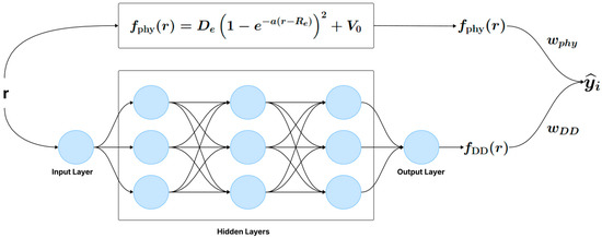
Figure 1.
One-step hybrid model (e.g., APHYNITY, PhysiNet).
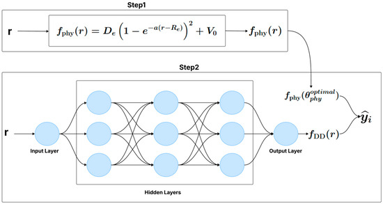
Figure 2.
Two-step hybrid model (e.g., Sequential Phy-ML).
2.2. Training, Hybrid Models, and Parametrization
2.2.1. Training
Training the hybrid models involves estimating the parameters of both the physical component () and the data-driven neural network (). Depending on the chosen approach, this optimization is performed either simultaneously or in two successive steps. In the one-step models, both sets of parameters are jointly updated using backpropagation, where the gradient of the combined loss function is computed and propagated through the entire model, allowing concurrent refinement of and (Algorithm 1). In contrast, the two-step model follows a sequential scheme: it first optimizes the physical parameters independently by minimizing a dedicated loss and subsequently fixes them to train the neural network on the residual error using standard backpropagation (Algorithm 2). These optimization procedures are described in detail in Section 2.2.2 and Section 2.2.3.
To achieve this, we use a finite dataset containing discrete values of potential energy (u.a.), corresponding to internuclear distances r (Å). These distances are uniformly discretized with a resolution of , covering the range .
| Algorithm 1 Training of the one-step models |
|
| Algorithm 2 Training of the two-step model |
|
2.2.2. One-Step Models
The one-step models apply the hybrid modeling principle in a single step, as presented in Algorithm 1. In the following sections, we describe the implementation of each model using this approach: APHYNITY and PhysiNet.
denotes the learning rate, which controls the step size of the gradient descent updates, while is the total number of training iterations. To determine the optimal values of both and for each training data size and for each potential energy curve considered, we performed a grid search over predefined ranges. The selected values aim to ensure stable and efficient convergence of the training process. The specific values used in each case are reported in Appendix A. L denotes the loss function (see each method below for its definition).
APHYNITY model
APHYNITY [29] was initially developed to address a widespread issue across many scientific fields: forecasting complex dynamical phenomena in situations where only partial knowledge of the underlying dynamics is available. Purely data-driven approaches are often insufficient in such cases, while purely physics-based models, being overly simplistic, tend to introduce significant errors. APHYNITY offers a rigorous hybrid approach that combines an incomplete physical model (formulated through differential equations) with a neural component that learns only the aspects not captured by the physics. In our work, we adapted this framework to our specific need for predicting potential energy surfaces.
APHYNITY implements the hybrid model principle in a single step, as shown in Algorithm 1, and taking = = 1, as follows:
The loss function L serves two purposes: it minimizes the overall error of the combined model , which measures the accuracy of the combined prediction , and it strengthens the influence of the physical model through a penalty term scaled by .
The parameter plays a crucial role in balancing the contributions of the physical and neural components of the model. Increasing strengthens the influence of the penalty term associated with the physical model , encouraging the training process to stay closer to the prior physical knowledge. Conversely, a smaller value of allows the neural component more flexibility to correct discrepancies not captured by the physical model. In this study, was empirically adjusted based on the training batch size (see Appendix A). This tuning helps to strike an optimal trade-off between adherence to the physical model and adaptability to the data.
PhysiNet model
PhysiNet [30] was initially developed to address the challenge of accurately modeling newly designed physical systems, where available data are limited, and physics-based models are often only approximate. The original goal of PhysiNet was to combine these two modeling paradigms in a hybrid approach that leverages their respective strengths. We later adapted PhysiNet to our specific context of predicting potential energy curves.
PhysiNet implements the hybrid model principle in a single step, as shown in Algorithm 1. Here, and are weighting coefficients that balance the contributions of the physics-based model and the data-driven model, respectively. These weights are initialized at 0.99 and 0.01 and are adjusted over epochs to optimize predictions, ensuring an adaptive balance between the two approaches. To achieve this, the model is trained using the following loss function:
2.2.3. Two-Step Model
Sequential model
This hybrid model follows a two-step approach, as described in Algorithm 2. The hyperparameters and represent the learning rates used in the two sequential training steps. Specifically, is the learning rate for optimizing the parameters of the physical model during the first phase, while is used in the second phase to train the neural network that corrects the residual error. These values were tuned using a grid search procedure to ensure the optimal convergence for both components of the model. The selected values for and are reported in Appendix A.
In the first phase, the parameters of the physical model are optimized to minimize the error between the physical model’s predictions and the target values . This optimization is performed by minimizing the following loss function:
Once the optimal physical parameters are obtained, they are kept fixed, and a neural network is trained to refine the predictions by minimizing the remaining residual error. The loss function used in this second phase is defined as follows:
3. Evaluation
Before evaluating the models quantitatively, we first illustrate the target potential energy curves used in this study (Figure 3). These include the ground state and the first excited state energy curves of , which serve as the reference for model predictions. The curves were computed using full configuration interaction as implemented in the GAMESS-US ab-initio program [31]. The aug-cc-pVDZ basis set was employed [32,33]. The codes and ab initio potential energy curves are available here:1.
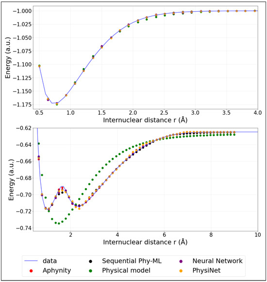
Figure 3.
Model predictions of PECs: ground state (top panel) and first excited state; (bottom panel). (The training was performed using 20% of the data).
We mention here that we employ adiabatic potential energy curves. The first excited state clearly exhibits an avoided crossing with a higher excited state. A diabatic representation would be necessary to perform meaningful molecular dynamics simulations. However, our aim is to investigate how hybrid models perform to predict a complex potential energy curve. The adiabatic representation is therefore sufficient.
The colored points represent the predicted energies obtained from the models described in the previous section. These models were trained using only 20% (corresponding to 32 points) of the available data. For comparison, Appendix B provides similar plots where the models were instead trained on 40% (corresponding to 64 points) of the data, illustrating the impact of additional training information on the prediction accuracy.
3.1. Root Mean Square Error
We evaluate the model predictions on the potential energy surface by computing the Root Mean Square Error (RMSE), which measures the difference between the predicted and actual values.
To evaluate the models’ performance as a function of the training dataset size, the models were trained on increasing fractions of the dataset: 5%, 10%, 15%, 20%, 25%, 30%, 35%, and 40% (corresponding to 8, 16, 24, 32, 40, 48, 56, and 64 data points, respectively), with each training run being independent. Importantly, each data subset is cumulative: for example, the 40% dataset includes all data points present in the smaller subsets. The remaining data, not used for training, were set aside for testing.
For each data fraction, training was repeated using different random initializations (Seed = 2, 4, 10, 22, 23, 28, 29, 30, 32, 42, 52) to assess the models’ robustness to randomness. Performance analysis is based on comparing the median RMSE values 2 across training batches, providing a reliable evaluation of each model’s performance.
To better understand the variability and consistency of the model performance across multiple training runs, we compute also the first and third quartiles (3 and 4). These statistical measures provide insights into the dispersion of the prediction errors, allowing us to assess how stable or sensitive the model is to different random initializations. A narrow gap between these quartiles indicates consistent performance across training runs, while a wider gap suggests greater variability.
All statistical analyses were conducted using Python 3.6 programming. They are defined as below:
3.2. Franck–Condon Factors
In addition to the statistical evaluation based on the RMSE, we also calculated the Franck–Condon factors (FCf) to assess the quality of the PECs. This approach goes beyond a simple numerical comparison between predicted and actual values by considering the physical relevance of the obtained curves. Thus, the use of Franck–Condon factors provides an additional validation, ensuring that the predicted curves accurately reflect the expected molecular properties.
The Franck–Condon factors measure the overlap between two vibrational wavefunctions corresponding to different electronic states of a molecule. A high FCf indicates strong overlap between the wavefunctions, making the transition more likely, while a low FCf suggests a less probable transition. They are given by
In our case, we have considered the following: the first vibrational wavefunction of the ground state and one vibrational wavefunction of the first excited state. The Franck–Condon factors depend strongly on the accuracy of the potential energy curves. They, therefore, provide a global estimate of the accuracy of the latter computed within each model.
In this study, we used the potential energy curves generated by the models with different random seeds (2, 4, 10, 22, 23, 28, 29, 30, 32, 42, 52) to compute the k Franck–Condon factors for each run. The accuracy of the predicted potential energy curves was evaluated by comparing the FCf values obtained from each seed with the corresponding reference values, using the as the performance metric:
To provide a robust evaluation of the Franck–Condon factors predicted by each model, we compute the mean square error between the predicted and reference FCf values for each random seed and report the median of these MSE values (), along with the first () and third () quartiles. These statistics offer insight into the stability and variability of the FCf predictions across different random initializations.
4. Results
4.1. Evaluation Using RMSE on the Testing Set
We analyze and discuss below the results obtained for the reconstruction of the potential energy curve of for the ground state and the first excited state. We mention here that each state is considered separately.
We compare the median RMSE values for five models—APHYNITY, Sequential Phy-ML, PhysiNet, a neural network, and the Morse potential—used to predict the potential energy as a function of the internuclear distance. Figure 4 corresponds to the ground state, while Figure 5 shows the results for the first excited state.
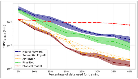
Figure 4.
as a function of the training set size for the ground state of .
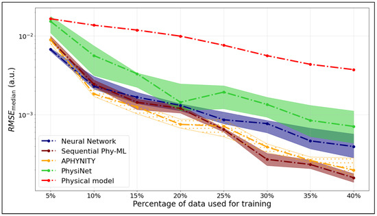
Figure 5.
as a function of the training set size for the first excited state of .
The x-axis represents the percentage of the dataset used for training, while the y-axis shows the values calculated on the testing data. The hatched areas around the curves indicate the interquartile range ( to ), which describes the variability of the models’ performance across these runs.
We observed for the potential energy curve of the ground state that the hybrid models, APHYNITY and Sequential Phy-ML, exhibit performance comparable to that of the physical model when trained on the smallest dataset (5%), relying primarily on the prior knowledge it provides. However, as more data become available, they surpass not only the physical model but also the neural network. This progression highlights their ability to leverage both physical knowledge and statistical learning. The PhysiNet model exhibits performance comparable to that of the neural network when trained on a small dataset, relying primarily on statistical learning. However, as the dataset expands, it utilizes the available information more effectively. By incorporating the prior knowledge from the physical model, it ultimately surpasses the prediction quality of the neural network.
For the potential energy curve of the first excited state, we observe a general decrease in as the percentage of training data increases, which is expected. The physical model consistently underperforms compared to the others, showing significantly higher RMSE values. In contrast, the APHYNITY, Sequential Phy-ML, and neural network models exhibit comparable and much better performance, especially beyond 30% of the training data, with a slight advantage for the Sequential Phy-ML model at higher data percentages. During the prediction of the first excited state curve, both hybrid models—APHYNITY and Sequential Phy-ML—show performance similar to that of the neural network when training is performed on less than 25% of the data. This can be explained by the fact that the physical model does not provide a sufficient prior, as it presents only a single minimum, whereas the target curve has two. Consequently, the hybrid models require more training data to adjust the discrepancy between the physical model and the target curve, compared to the ground state.
4.2. Evaluation Using on the Test Set
Figure 6 shows the evolution of the mean square error computed on the Franck–Condon factors () as a function of the percentage of data used for training, for different models. Each curve represents the median across different random seeds. The shaded areas correspond to the interquartile range, i.e., the region between the first () and third () quartiles.
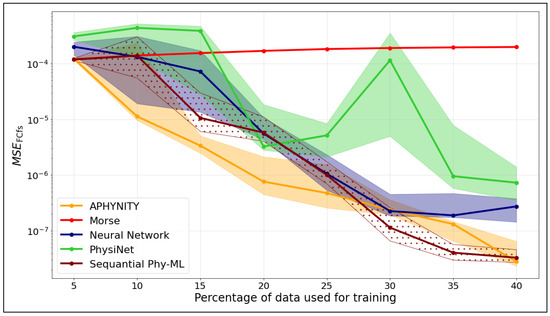
Figure 6.
as a function of the training set size of .
We observe that the Franck–Condon factors obtained from the APHYNITY model consistently have a lower than those obtained from the neural network, regardless of the training set size.
The Sequential Phy-ML model requires more data to accurately construct the eigenvectors used in the calculation of the Franck–Condon factors. From a training set representing 30% of the data, we observe that the Franck–Condon factors obtained with the Sequential Phy-ML model exhibit a lower than those obtained from the neural network.
In comparison, the Morse model shows stable but limited improvement with increasing data, which is expected given its analytical formulation. PhysiNet performs well at low data fractions but displays notable variability, particularly between 25% and 30%. The neural network model shows steady improvement as more data are provided, yet its performance remains less consistent than that of the hybrid approaches.
4.3. Comparison of the Obtained Physical Parameters
Table 1 shows the deviation between the physical parameters (De, a, and Re) estimated using hybrid-residual models (APHYNNITY, Sequential Phy-ML, and PhysiNet) and the values obtained from the Morse model. These deviations are reported for different training data sizes (ranging from 5% to 40%) and allow us to assess the ability of the models to recover the physical parameters with varying amounts of data. For each model and configuration, the errors are reported for three different random seeds (2, 22, and 42) to evaluate the variability due to the random initialization of the neural network.

Table 1.
Deviation of the estimated physical parameters from the physical model values.
Among the three hybrid models studied, APHYNITY and the Sequential Phy-ML model stand out for their ability to reliably predict the physical parameters of the Morse potential, even when the training dataset is limited in size. This can be attributed to the way these two approaches explicitly incorporate the physical model into the training process. In particular, APHYNITY applies a direct penalty on the error of the physical model, which strongly constrains the predictions to remain close to the underlying physical reality. Similarly, the Sequential Phy-ML model first optimizes the physical parameters independently, before training a neural network on the residual error. This two-step process helps maintain a good approximation of the physical parameters.
In contrast, PhysiNet performs significantly worse when it comes to predicting the physical parameters. Although this model also adopts a hybrid approach, it does not constrain the physical component during training. The weights assigned to the physical and neural components are adjusted adaptively, but this flexibility can quickly lead to a weakened influence of the physical model, especially if the neural network overcorrects the errors. As a result, the physical parameters may drift toward unrealistic values.
5. Conclusions
This paper presented a comparative study of three hybrid models—APHYNITY, Sequential Phy-ML, and PhysiNet—which combine physical knowledge with machine learning for the reconstruction of potential energy curves. The ground and first excited states of the hydrogen molecule are used as examples to illustrate the methods and results. The two different potential energy curves provide a benchmark for the hybrid approaches and allow deeply understanding the capabilities and limitations of the methods. They, therefore, provide useful and general insights into the use of hybrid approaches for predicting potential energy surfaces.
The main findings are as follows:
- When only a limited amount of data is available, hybrid models outperform purely neural network approaches, thanks to the structural guidance provided by the physical model. However, in cases where the physical model is not very informative, hybrid models only become competitive once a sufficient volume of data is provided.
- The use of Franck–Condon factors as an evaluation criterion confirmed that hybrid models, particularly APHYNITY and Sequential Phy-ML, produce curves that are more physically consistent than those generated by neural networks.
These results highlight the value of hybrid approaches for accurately modeling complex molecular systems. It should be noted that the computational costs for training the models are fairly low. The calculations were performed on a standard laptop (Intel Core i5, 8 GB of RAM). Each training takes between a few seconds and half an hour depending on the method and size of the training dataset. Furthermore, the training computational costs, as well as the performance of each model, should not depend significantly on the molecular system under consideration. Indeed, the methods we investigated rely only on the shape of the potential energy curves. Similar results should therefore be obtained for other diatomic molecules or for bond stretching modes of poly-atomic molecules. Covalent bonds are usually well described by a Morse potential. For ionic bonds or Van der Waals interactions, the hybrid approaches should still provide accurate results thanks to the data-driven part. However, the use of other physics-based potentials would be more efficient.
Future directions may include adapting these models to larger systems, for example triatomic molecules, as well as the use of different physics-based models (i.e., other than a Morse potential) or exploring the use of Physics-Informed Neural Networks (PINNs) for reconstructing potential energy curves.
Author Contributions
Conceptualization, K.E.H., N.T. and N.S.; methodology, K.E.H., N.T. and N.S.; software, K.E.H.; validation, K.E.H., N.T. and N.S.; formal analysis, K.E.H., N.T. and N.S.; investigation, K.E.H.; data curation, K.E.H.; writing—original draft preparation, K.E.H. and N.S.; writing—review and editing, K.E.H., N.T. and N.S.; supervision, N.T. and N.S.; project administration, N.T. and N.S.; funding acquisition, N.T. and N.S. All authors have read and agreed to the published version of the manuscript.
Funding
This research received no external funding.
Institutional Review Board Statement
Not applicable.
Informed Consent Statement
Not applicable.
Data Availability Statement
The codes and ab initio potential energy curves are available here: https://github.com/Kaoutar142/Combining-Physics-and-ML-for-predicting-interatomic-potentials.git.
Acknowledgments
This work was supported by the Sorbonne Center for Artificial Intelligence (SCAI), an institute dedicated to artificial intelligence within the Sorbonne University Alliance, funded by the excellence initiative IDEX SUPER under the ANR reference: 11-IDEX-0004. N.S. acknowledges support from the COST Action CA20129 MultIChem.
Conflicts of Interest
The authors declare no conflicts of interest.
Appendix A
Table A1.
Training parameters for ground state (APHYNITY).
Table A1.
Training parameters for ground state (APHYNITY).
| Training Data Size | Learning Rate | Penalty Factor | Number of Epochs |
|---|---|---|---|
| 5% | 0.0015 | 2 | 500,000 |
| 10% | 0.00098 | 6 | 500,000 |
| 15% | 0.001 | 6 | 500,000 |
| 20% | 0.00098 | 6 | 500,000 |
| 25% | 0.0007 | 3 | 1,200,000 |
| 30% | 0.0007 | 3 | 1,200,000 |
| 35% | 0.0007 | 3 | 1,200,000 |
| 40% | 0.0007 | 4 | 1,400,000 |
Table A2.
Training parameters for first excited state (APHYNITY).
Table A2.
Training parameters for first excited state (APHYNITY).
| Training Data Size | Learning Rate | Penalty Factor | Number of Epochs |
|---|---|---|---|
| 5% | 0.001 | 1 | 200,000 |
| 10% | 0.00098 | 6 | 200,000 |
| 15% | 0.00098 | 6 | 400,000 |
| 20% | 0.0009 | 6 | 400,000 |
| 25% | 0.0006 | 6 | 700,000 |
| 30% | 0.0006 | 6 | 700,000 |
| 35% | 0.00062 | 6 | 700,000 |
| 40% | 0.0007 | 4 | 900,000 |
Table A3.
Training parameters for ground state (PhysiNet).
Table A3.
Training parameters for ground state (PhysiNet).
| Training Data Size | Learning Rate | Number of Epochs |
|---|---|---|
| 5% | 0.00001 | 200,000 |
| 10% | 0.00001 | 200,000 |
| 15% | 0.00001 | 400,000 |
| 20% | 0.00001 | 400,000 |
| 25% | 0.000009 | 900,000 |
| 30% | 0.000009 | 900,000 |
| 35% | 0.000009 | 900,000 |
| 40% | 0.000009 | 900,000 |
Table A4.
Training parameters for first excited state (PhysiNet).
Table A4.
Training parameters for first excited state (PhysiNet).
| Training Data Size | Learning Rate | Number of Epochs |
|---|---|---|
| 5% | 0.00001 | 900,000 |
| 10% | 0.00001 | 900,000 |
| 15% | 0.00001 | 900,000 |
| 20% | 0.00001 | 900,000 |
| 25% | 0.000009 | 1,400,000 |
| 30% | 0.000009 | 1,400,000 |
| 35% | 0.000009 | 1,400,000 |
| 40% | 0.000009 | 1,400,000 |
Table A5.
Training parameters for ground state (Sequential Phy-ML).
Table A5.
Training parameters for ground state (Sequential Phy-ML).
| Training Data Size | Learning Rate | Number of Epochs |
|---|---|---|
| All size | 0.01 | 100,000 |
| All size | 0.0005 | 900,000 |
Table A6.
Training parameters for first excited state (Sequential Phy-ML).
Table A6.
Training parameters for first excited state (Sequential Phy-ML).
| Training Data Size | Learning Rate | Number of Epochs |
|---|---|---|
| All size | 0.01 | 100,000 |
| 5% to 20% | 0.001 | 100,000 |
| 20% to 40% | 0.00092 | 400,000 |
Appendix B

Figure A1.
Model predictions of PECs: ground state (Top panel) and first excited state (Bottom panel). (The training was performed using 40% of the data).
Figure A1.
Model predictions of PECs: ground state (Top panel) and first excited state (Bottom panel). (The training was performed using 40% of the data).

Notes
| 1 | Available online: https://github.com/Kaoutar142/Combining-Physics-and-ML-for-predicting-interatomic-potentials.git (accessed on 13 October 2025). |
| 2 | corresponds to the RMSE for which 50% of the training runs yield an error that is less than or equal to it, while the other 50% yield an error that is greater than or equal to it. This measure provides a more representative evaluation of the model’s overall performance across all trials. |
| 3 | The first quartile corresponds to the RMSE value below which 25% of the training runs fall. In other words, 25% of the RMSE values are less than or equal to this value, while 75% are greater. |
| 4 | The third quartile corresponds to the RMSE value below which 75% of the training runs fall. That is, 75% of the RMSE values are less than or equal to this value, while 25% are greater. |
References
- Ramakrishnan, R.; Hartmann, M.; Tapavicza, E.; von Lilienfeld, O.A. Electronic spectra from TDDFT and machine learning in chemical space. J. Chem. Phys. 2015, 143, 084111. [Google Scholar] [CrossRef]
- Pronobis, W.; Schütt, K.T.; Tkatchenko, A.; Müller, K.-R. Capturing intensive and extensive DFT/TDDFT molecular properties with machine learning. Eur. Phys. J. 2018, 91, 178. [Google Scholar] [CrossRef]
- Roy, R.L.; Henderson, R.D.E. A new potential function form incorporating extended long-range behaviour: Application to ground-state Ca2. Mol. Phys. 2018, 105, 663–677. [Google Scholar] [CrossRef]
- Roy, R.L.; Haugen, C.C.; Tao, J.; Li, H. Long-range damping functions improve the short-range behaviour of ’MLR’ potential energy functions. Mol. Phys. 2011, 109, 435–446. [Google Scholar] [CrossRef]
- Zhai, Y.; Li, H.; Roy, R.L. Constructing high-accuracy intermolecular potential energy surface with multi-dimension Morse/Long-Range model. Mol. Phys. 2018, 116, 843–853. [Google Scholar] [CrossRef]
- Behler, J. Neural network potential-energy surfaces in chemistry: A tool for large-scale simulations. Phys. Chem. Chem. Phys. 2011, 13, 17930–17955. [Google Scholar] [CrossRef]
- Hornik, K.; Stinchcombe, M.; White, H. Multilayer feedforward networks are universal approximators. Neural Netw. 1989, 2, 359–366. [Google Scholar] [CrossRef]
- Barron, A.R. Universal Approximation Bounds for Superpositions of a Sigmoidal Function. IEEE Trans. Inf. Theory 1993, 39, 930. [Google Scholar] [CrossRef]
- Manzhos, S.; Carrington, T., Jr. Neural Network Potential Energy Surfaces for Small Molecules and Reactions. Phys. Chem. Chem. Phys. 2021, 121, 10187–10217. [Google Scholar] [CrossRef]
- Dral, P.O. Quantum Chemistry in the Age of Machine Learning. J. Phys. Chem. Lett. 2020, 11, 2336–2347. [Google Scholar] [CrossRef]
- Jiang, B.; Li, J.; Guo, H. High-Fidelity Potential Energy Surfaces for Gas-Phase and Gas–Surface Scattering Processes from Machine Learning. J. Phys. Chem. Lett. 2020, 13, 5120–5131. [Google Scholar] [CrossRef]
- Meuwly, M. Machine Learning for Chemical Reactions. Chem. Rev. 2021, 121, 10218–10239. [Google Scholar] [CrossRef]
- Deringer, V.L.; Bartók, A.P.; Bernstein, N.; Wilkins, D.M.; Ceriotti, M.; Csányi, G. Gaussian Process Regression for Materials and Molecules. Chem. Rev. 2021, 121, 10187–10217. [Google Scholar] [CrossRef]
- Ye, S.; Hu, W.; Li, X.; Zhang, J.; Zhong, K.; Zhang, G.; Luo, Y.; Mukamel, S.; Jiang, J. A neural network protocol for electronic excitations of N-methylacetamide. Natl. Libr. Med. 2019, 116, 11612–11617. [Google Scholar] [CrossRef] [PubMed]
- Chen, W.K.; Liu, X.Y.; Fang, W.H.; Dral, P.O.; Cui, G. Deep Learning for Nonadiabatic Excited-State Dynamics. J. Phys. Chem. Lett. 2018, 9, 6702–6708. [Google Scholar] [CrossRef] [PubMed]
- Dral, P.O.; Barbatti, M.; Thiel, W. Nonadiabatic Excited-State Dynamics with Machine Learning. J. Phys. Chem. Lett. 2018, 9, 5660–5663. [Google Scholar] [CrossRef] [PubMed]
- Hu, D.; Xie, Y.; Li, X.; Li, L.; Lan, Z. Inclusion of Machine Learning Kernel Ridge Regression Potential Energy Surfaces in On-the-Fly Nonadiabatic Molecular Dynamics Simulation. J. Phys. Chem. Lett. 2018, 9, 2725–2732. [Google Scholar] [CrossRef]
- Westermayr, J.; Gastegger, M.; Menger, M.F.S.J.; Mai, S.; González, L.; Marquetand, P. Machine learning enables long time scale molecular photodynamics simulations. Chem. Sci. 2019, 10, 8100–8107. [Google Scholar] [CrossRef]
- Dral, P.O.; Barbatti, M. Molecular excited states through a machine learning lens. Nat. Rev. Chem. 2021, 5, 388–405. [Google Scholar] [CrossRef]
- Westermayr, J.; Marquetand, P. Deep learning for UV absorption spectra with SchNarc: First steps toward transferability in chemical compound space. J. Chem. Phys. 2020, 153, 154112. [Google Scholar] [CrossRef]
- Westermayr, J.; Faber, F.A.; Christensen, A.S.; von Lilienfeld, O.A.; Marquetand, P. Neural networks and kernel ridge regression for excited states dynamics of CH2NH2: From single-state to multi-state representations and multi-property machine learning models. Mach. Learn. Sci. Technol. 2020, 1, 025009. [Google Scholar] [CrossRef]
- Li, A.; Guo, H. A full-dimensional global potential energy surface of H3O+(ã3A) for the OH+(3Σ−) + H2(1Σg+) → H(2S) + H2O+(2B1) reaction. J. Phys. Chem. A 2014, 118, 11168–11176. [Google Scholar] [CrossRef]
- Stoppelman, J.P.; McDaniel, J.G. Physics-based, neural network force fields for reactive molecular dynamics: Investigation of carbene formation from [EMIM+][OAc−]. Chem. Phys. 2021, 155, 104112. [Google Scholar] [CrossRef]
- Bereau, T.; DiStasio, R.A., Jr.; Tkatchenko, A.; von Lilienfeld, O.A. Non-covalent interactions across organic and biological subsets of chemical space: Physics-based potentials parametrized from machine learning. Chem. Phys. 2018, 148, 241706. [Google Scholar] [CrossRef]
- Konrad, M.; Wenzel, W. CONI-Net: Machine Learning of Separable Intermolecular Force Fields. J. Chem. Theory Comput. 2021, 17, 4996–5006. [Google Scholar] [CrossRef]
- Ramakrishnan, R.; Dral, P.O.; Rupp, M.; von Lilienfeld, O.A. Big Data Meets Quantum Chemistry Approximations: The Δ-Machine Learning Approach. J. Chem. Theory Comput. 2015, 11, 2087–2096. [Google Scholar] [CrossRef]
- Westermayr, J.; Gastegger, M.; Schütt, K.T.; Maurer, R.J. Perspective on integrating machine learning into computational chemistry and materials science. J. Chem. Phys. 2021, 154, 230903. [Google Scholar] [CrossRef]
- Li, S.; Xie, B.B.; Yin, B.W.; Liu, L.; Shen, L.; Fang, W.H. Construction of Highly Accurate Machine Learning Potential Energy Surfaces for Excited-State Dynamics Simulations Based on Low-Level Data Sets. J. Phys. Chem. A 2024, 128, 5516–5524. [Google Scholar] [CrossRef]
- Yin, Y.; Guen, V.L.; Dona, J.; de Bézenac, E.; Ayed, I.; Thome, N.; Gallinari, P. Augmenting Physical Models with Deep Networks for Complex Dynamics Forecasting. J. Stat. Mech. Theory Exp. 2021, 2021, 124012. [Google Scholar] [CrossRef]
- Sun, C.; Shi, V.G. PhysiNet: A Combination of Physics-based Model and Neural Network Model for Digital Twins. Int. J. Intell. Syst. 2021, 37, 5443–5456. [Google Scholar] [CrossRef]
- Schmidt, M.W.; Baldridge, K.K.; Boatz, J.A.; Elbert, S.T.; Gordon, M.S.; Jensen, J.H.; Koseki, S.; Matsunaga, N.; Nguyen, K.A.; Su, S.; et al. General atomic and molecular electronic structure system. J. Comput. Chem. 1993, 14, 1347–1363. [Google Scholar] [CrossRef]
- Dunning, T.H. Gaussian basis sets for use in correlated molecular calculations. I. The atoms boron through neon and hydrogen. J. Chem. Phys. 1989, 90, 1007–1023. [Google Scholar] [CrossRef]
- Kendall, R.A.; Dunning, T.H.; Harrison, R.J. Electron affinities of the first-row atoms revisited. Systematic basis sets and wave functions. J. Chem. Phys. 1992, 96, 6796–6806. [Google Scholar] [CrossRef]


Disclaimer/Publisher’s Note: The statements, opinions and data contained in all publications are solely those of the individual author(s) and contributor(s) and not of MDPI and/or the editor(s). MDPI and/or the editor(s) disclaim responsibility for any injury to people or property resulting from any ideas, methods, instructions or products referred to in the content. |
© 2025 by the authors. Licensee MDPI, Basel, Switzerland. This article is an open access article distributed under the terms and conditions of the Creative Commons Attribution (CC BY) license (https://creativecommons.org/licenses/by/4.0/).