Abstract
Recent advancements in studying long chains of unstable nuclei have revitalised interest in investigating the hyperfine anomaly. Hyperfine anomaly is particularly relevant for determining nuclear magnetic dipole moments using hyperfine structures where it limits the accuracy. This research paper focuses on the calculation of the differential Breit-Rosenthal effect for the , and states in Pb, utilising the multi-configurational Dirac-Hartree-Fock code, GRASP2018. The findings show that the differential Breit-Rosenthal effect is typically less than , which is often much smaller than the Bohr-Weisskopf effect. The differential Breit-Rosenthal effect for the state is one order of magnitude smaller than the rest, which is why this state seems to be insensible to the hyperfine anomaly.
1. Introduction
Nuclear magnetic moments play a crucial role in understanding the fundamental structure of the nucleus. They have significant implications not only in basic nuclear research but also in various other research fields such as atomic physics, chemistry, and solid-state physics. The electric quadrupole moment is associated with the nuclear charge distribution’s shape, while the magnetic dipole moment relates to the angular momentum of the nucleus.
Throughout the years, diverse techniques have been developed to determine experim- ental values of nuclear moments for both stable and unstable nuclei [1]. For magnetic dipole moment determination, many methods require corrections for the effects of the medium on an applied magnetic field, like diamagnetism, Knight shift, and the hyperfine anomaly (hfa) [2,3]. The corrections introduce limitations to the uncertainty of the experimental values. In this study, we specifically focus on the corrections resulting from the non-point-like nature of the nucleus, i.e., the hyperfine anomaly.
The hyperfine anomaly, , is normally defined as:
where the ratio of measured hyperfine structure constants (a) for two isotopes is compared with the independently measured ratio of nuclear magnetic dipole moments () and nuclear spins (I) for isotopes 1 and 2.
While anomalies in the first order can usually be disregarded for electrons with total angular momentum j > 1/2 due to vanishing wavefunctions at the nucleus, higher-order electronic correlations can lead to substantial anomalies in certain cases, such as in states [3].
The hyperfine anomaly is composed of two parts: the Bohr-Weisskopf effect (BW-effect) [2,4,5], related to the magnetization distribution in the nucleus, and the Breit-Rosenthal effect (BR-effect) [6,7,8,9], associated with the extended charge distribution of the nucleus.
Bohr and Weisskopf [4] considered the influence of the finite size of the nucleus, i.e., the distribution of magnetization on the hyperfine structure. They showed that the magnetic dipole hyperfine interaction constant (a) for an extended nucleus is generally smaller than the value expected for a point nucleus. The hyperfine interaction constant is expressed as:
where is the BW-effect, and is the hyperfine interaction constant for a point-like nucleus.
The Breit-Rosenthal effect (BR-effect) arises from the extended charge distribution of the nucleus [6,7,8,9], and its absolute value can reach up to 25%. Thus, the hyperfine interaction constant (a) can be written as:
To compare isotopes of an element and focus on the differential effect, we express the hfa as:
In this context, we are particularly interested in the differential Breit-Rosenthal effect (BR-anomaly) (), which is considered to be relatively small, around for isotope pairs. However, when studying long chains of isotopes, significant changes in nuclear charge distribution, especially at shape transitions, become relevant, underscoring the importance of systematic investigations of the differential BR-effect.
While the hyperfine anomaly (hfa) and the Bohr-Weisskopf effect have received some attention in the last two decades, the Breit-Rosenthal effect (BR-effect) has been less explored since Rosenberg and Stroke’s work in 1972 [9]. They calculated the BR-effect using diffuse and Hofstadter-type charge distributions for isotope pairs () in various elements. However, our focus lies in coupling the BR-anomaly () to the change in charge radius () to apply it across long chains of isotopes. The desired form to express the BR-anomaly is:
where the change in charge radius can be obtained from tables [10] or isotope shift studies.
This work is a continuation of the calculations of the BR-effect completed by Heggset and Persson in the states in Hg [11].
The objectives of this study are twofold. First, we aim to expand the data set of differential BR-effect as a function of changes in nuclear charge radius in heavy atoms, building on the results of Heggset et al. [11]. Second, we seek to explore the effect of extending the configuration expansion in Multi-Configurational Dirac-Hartree-Fock (MCDHF) calculations on the BR-anomaly, as this seemed to be relatively independent on the size of the expansions in Hg [11]. This will shed light on the extent of expansions required in the calculations for other heavy atoms.
2. MCDHF Method
The computations in this study were carried out using the Multi-Configurational Dirac-Hartree-Fock package, known as GRASP2018 [12]. This package is based on a combination of the MCDHF (Multi-Configurational Dirac-Hartree-Fock) and RCI (Relativistic Configuration Interaction) methods [13,14]. In this paper, we follow the procedure laid out in [12,15] and by Heggset et al. [11]. A detailed description of the calculations can be found in the master’s thesis of the first author [16].
The specific focus of this study lies on the spectroscopic states , and in Pb, with Pb () used as the reference isotope. The calculations utilized the tabulated values for the nuclear radius, with R = 5.4943(14) fm [10], and the nuclear moment, with a value of = 0.5925839(9) [17]. The experimental values used (Table 1) were taken from [18].

Table 1.
Magnetic hyperfine structure constants a of the Pb states.
Fermi Distribution
The charge distribution of the nucleus can be modelled in various ways. Rosenberg and Stroke [9] employed both a simple model with a homogeneous charge distribution and a Hofstadter distribution. A widely used and realistic model is the two-parameter Fermi distribution ([19] p. 27), which offers additional flexibility in calculations:
where c represents the half-density radius, and b is related to the so-called skin thickness t by . GRASP2018 enables the use of a two-parameter Fermi distribution to approximate the nuclear charge distribution.
The shape of the nuclear distribution, including the skin thickness, may be characterized by the expansion of moments of the distribution. Consequently, changes in nuclear size can be described using . However, given that the differential Breit-Rosenthal effect is expected to be small in comparison to the differential Bohr-Weisskopf effect and the uncertainty in the experimental data, it should be adequate to consider only the first term () and the skin thickness (t) in the expansion.
3. Calculations
Computations were mostly performed with the even parity and odd parity configurations together, although some single configuration calculations were also performed. When performing both configurations together, all spectroscopic orbitals achieved convergence together.
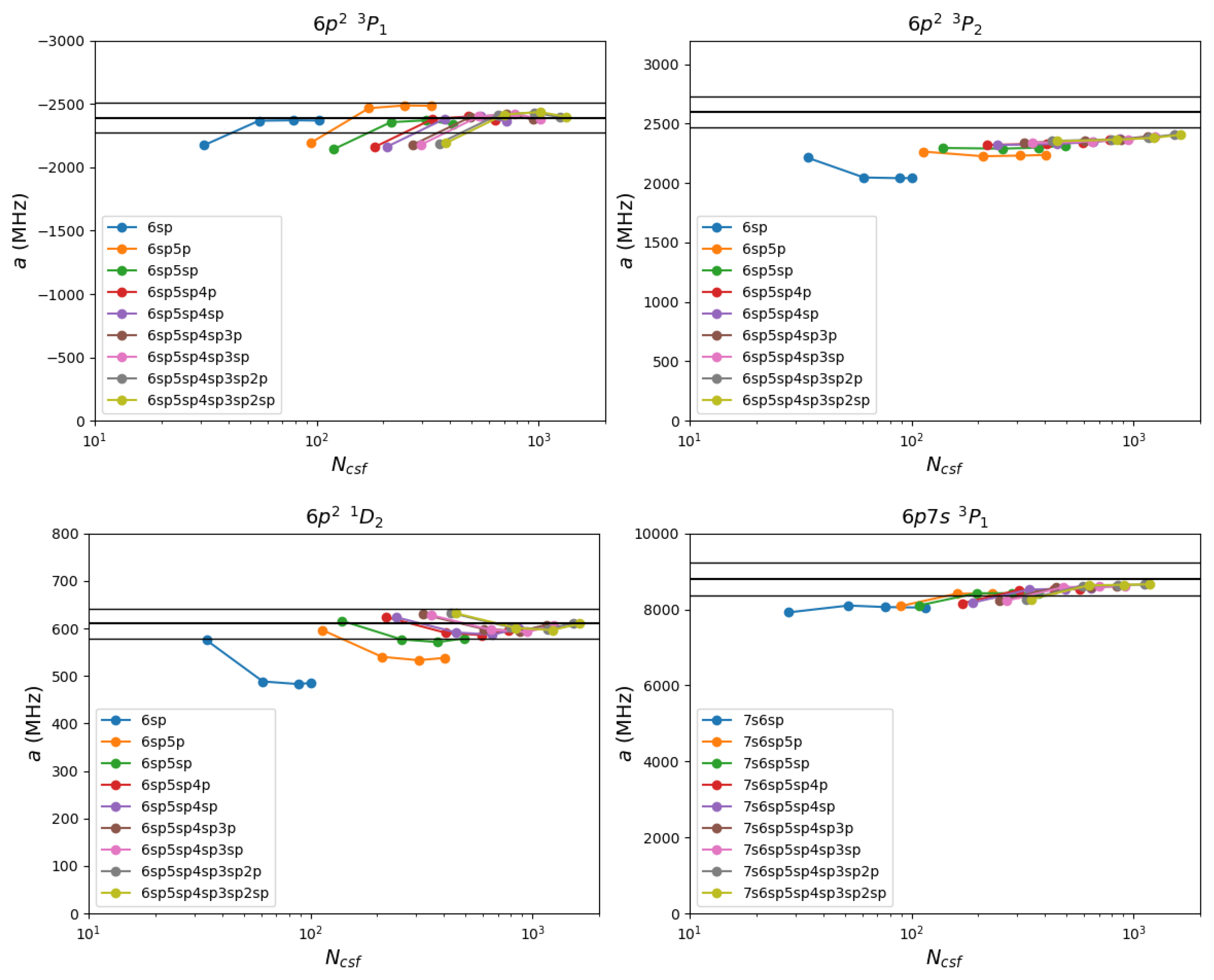
In the calculations, the active orbital sets were introduced layer-by-layer with optimiz- ation of each layer before the next was introduced. With subsequent smaller contributions of active orbitals, the total number of layers was limited to four layers ({8s 7p 6d 5f}, {9s 8p 7d 6f}, {10s 9p 8d 7f} and {11s 10p 9d 8f}) in the calculations as the contribution of additional layers is expected to be small. This can be observed in Figure 1.
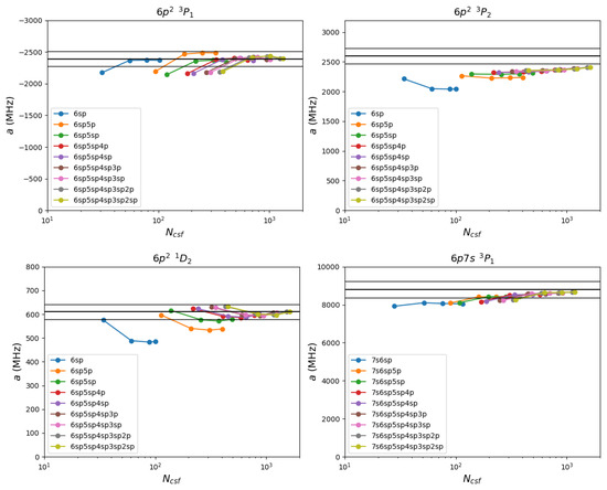
Figure 1.
Unrestricted single substitutions allowed. Each data series corresponds to one set of active peel subshells and the four data points in each series correspond to the first, …, fourth virtual layer. The horizontal black lines in each graph indicate the experimental value of a for the given state and a interval around the experimental value which serves as a guide to the eye of the quality of the calculation.
The hyperfine interaction is described by one-particle operators, so only CSFs corresp- onding to single (S) substitutions need to be included in the ASF expansion to first approximation [20]. Therefore, the bulk of the hyperfine structure was expected to be obtained in the calculations based on S substitutions. Substitutions from all active subshells were allowed to the four layers of virtual orbitals. The calculations started with small valence subshells , and before the core subshells were introduced in subsequent runs, in the order , , …, , .
After the optimization of each layer, the hyperfine structure constants were calculated. The results are presented in Figure 1.
As the active set was increased, a convergence toward the experimental a-value for all states was achieved. The results were excellent in and , good in and somewhat off in . This is an indication that correlation beyond the first approximation represented by single substitutions is of importance in the latter state. For all four states the final expansion, generated by allowing single excitations from to four layers of active orbitals gave the most accurate calculated a-value. The deviation from the experimental value of a for all states with single substitutions is given in Table 2.
Table 2.
Deviation in a-values for the expansion generated by single excitations from to four virtual layers, compared to the experimentally measured value . Here, .
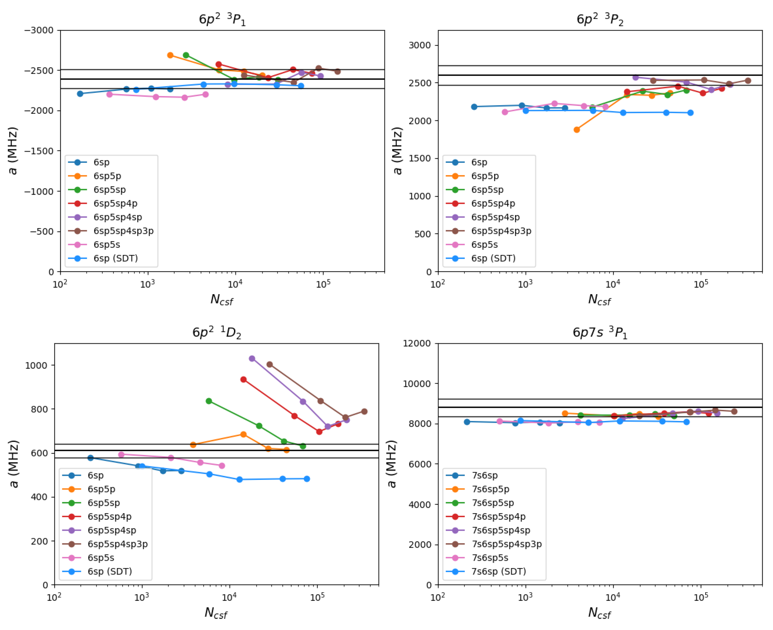
Since correlation effects are important, the calculations were expanded to also include double (D) substitutions. The procedure of S substitutions was repeated with D substitutions including valence-valence (vv), core-valence (cv) and core-core (cc) substitutions. The calculated a values as the active set increases are given in Figure 2.
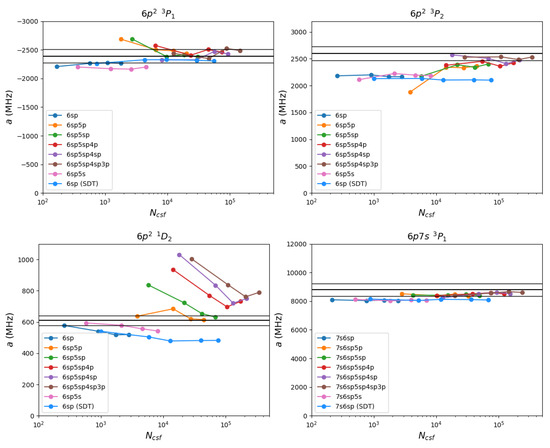
Figure 2.
Unrestricted single and double substitutions allowed, except one series with unrestricted single, double and triple substitutions. Each data series corresponds to one set of active peel subshells and the four (five) data points in each series correspond to the first, …, fourth (fifth) virtual layer. The horizontal black lines in each graph indicate the experimental value of a for the given state, and and a interval around the experimental value which serves as a guide to the eye of the quality of the calculation.
The calculations based on SD substitutions led to convergence towards the experimental value and yielded quite good results in all states except . The deviation between the experimental and calculated values of a using the biggest expansion is given in Table 3.
Table 3.
Deviation in a-values for the expansion generated by unrestricted SD excitations from to four virtual layers, compared to the experimentally measured value . Here, .
In SD excitations from core subshells cause an overestimation of the hyperfine structure which was not caused by single substitutions alone, showing the importance of cv and/or cc correlation. This trend is visible from activation of 5 s but recovers by the fourth virtual layer.
In terms of accuracy, only in was an improvement in the calculations based on single and double substitutions observed compared to the calculations based on single substitutions, indicating that vv and cv correlation is of importance in this state. It should also be noted that the state is sensitive to these correlations.
To test the higher order of correlations a calculation on unrestricted single, double and triple (SDT) substitutions were performed, only involving the valence , and orbitals. This was motivated by the rapidly increasing number of CSFs in the expansion, which was deemed unfeasible in this study. In this case we allowed an extra (fifth) virtual layer in the calculation. The results are included as a single series in Figure 2.
Including T substitutions did not alter the calculated a values substantially. This is in agreement with expectations, as CSFs generated by T substitutions correspond to higher-order corrections. Overall, the calculations based on SDT substitutions and only valence orbitals gave quite poor results, indicating that core polarization should be included. This is certainly the case for the and states. Table 4 shows the deviation between the calculated a-values for the expansion generated by SDT excitations from to five layers, relative to the experimental value.
Table 4.
Deviation in a-values for the expansion generated by SDT excitations from to five virtual layers, compared to the experimentally measured value . Here, .
Expansions for Calculations of the Breit-Rosenthal Effect
From the results of the calculations of the a-constant, the values obtained for the and are quite stable while the and varies for different expansions. The use of an extended core for triple substitutions might improve the values for these states, but this was not deemed sensible in this study. The main focus of this study is on the calculation of the Breit-Rosenthal effect and based on the results we choose to use five different expansions to investigate how much the different expansions affect the Breit-Rosenthal effect. This is to answer how large the expansions need to be to give a sensible value of the Breit-Rosenthal effect. The five expansions selected were:
- Unrestricted SD excitations allowed from .
- Unrestricted SDT excitations allowed from .
- Unrestricted SD excitations allowed from .
- Unrestricted SD excitations allowed from .
- Unrestricted S excitations allowed from .
4. Variations in Nuclear Radius
The calculations were performed over the range of all experimental values of the rms radii of lead isotopes given by Angeli and Marinova [10] and presently unmeasured isotopes. That is the range of deviation in the mean squared radius from the 207Pb reference isotope is between and , as calculated with the relation ([10] p. 2).
The calculations of the hfs constants followed the described procedure using the new nuclear parameters (radii). The obtained a for every value of was compared to the value for the reference isotope. With the obtained values of , the BR effect was approximated by the proportionality constant in the linear fit.
With all expansions and virtual layers a total of 20 values of were calculated using a linear regression with a no-intercept model, forcing the fit through the origin. In this model, was calculated as
where the sum is over the values corresponding to the set of nuclear radii.
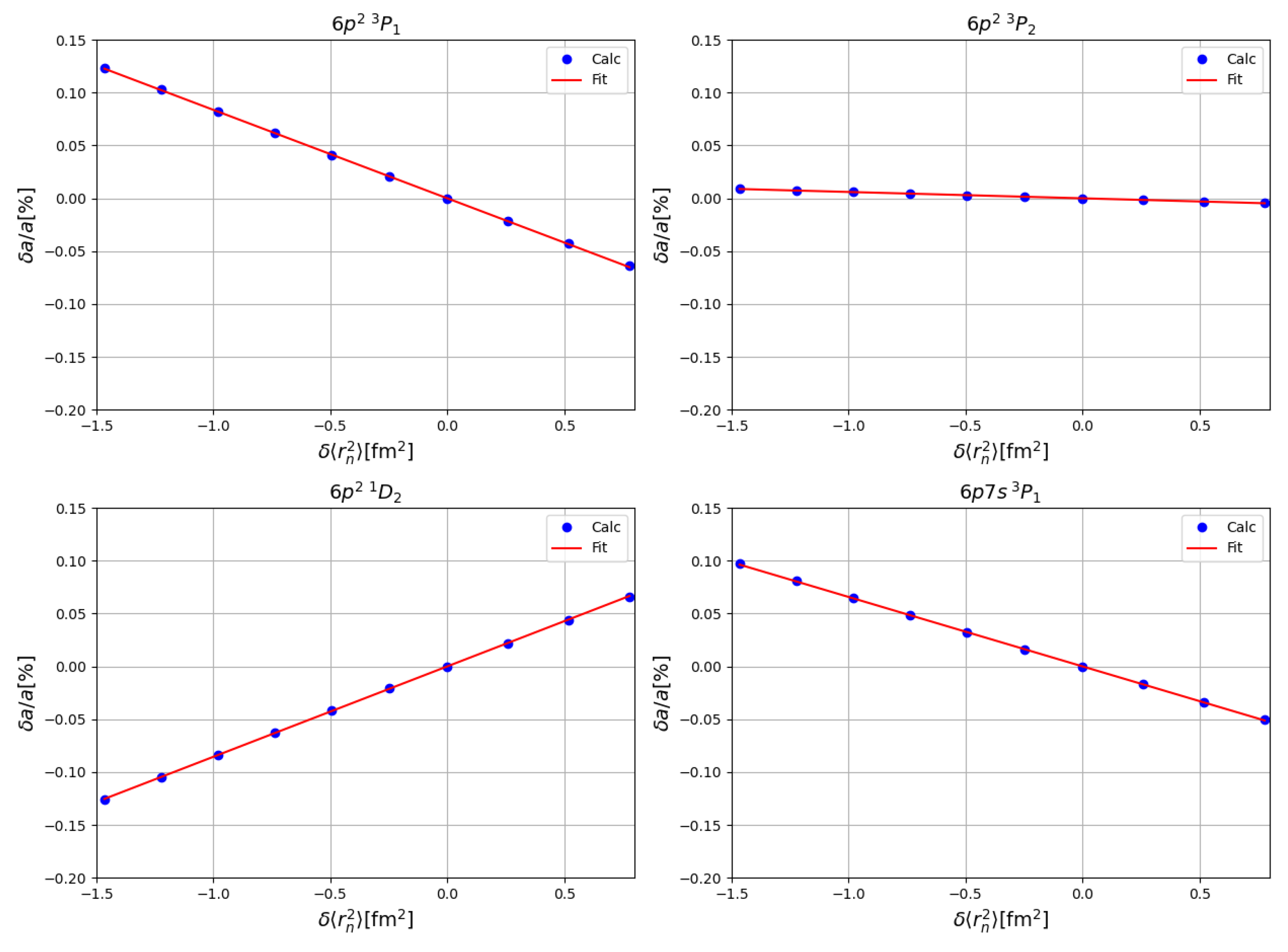
In Figure 3 an example is presented. Here, the data for the expansion created by allowing SD substitutions from the subshells is presented, alongside the calculated linear fit for each state.
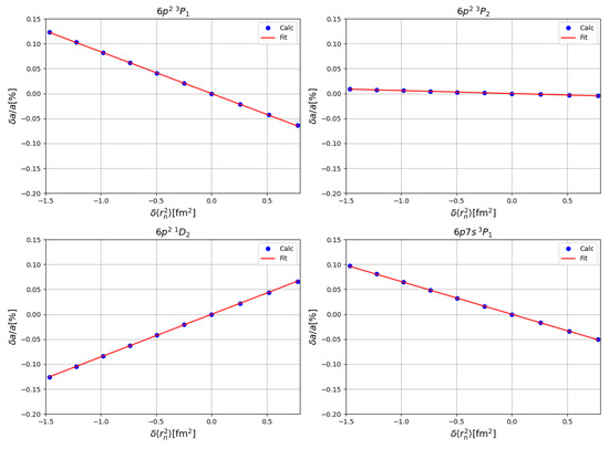
Figure 3.
Relative change in the hfs constant against deviation in the mean squared radius of the nuclear Fermi charge distribution from the reference nucleus with hfs constant . Based on the expansion generated with SD excitations from the subshells to four virtual layers. The red line represents the linear fit.
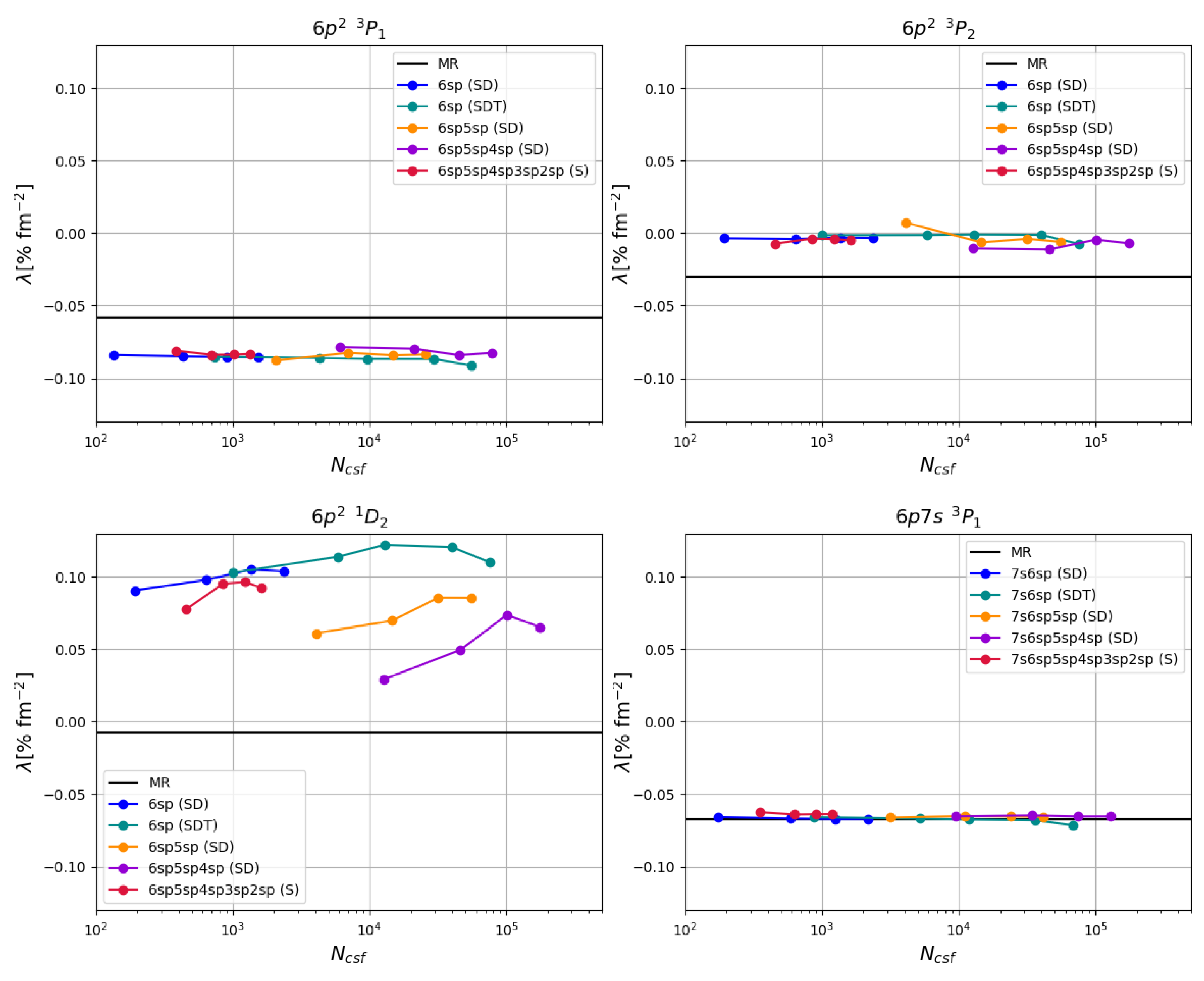
The constants for the BR effect are presented in Figure 4. The calculated proportionality constants change as the active set is increased. In addition, the value of calculated with the multireference CSFs is included for comparison. The coefficient of correlation for the obtained -values was except for SDT excitations from with .
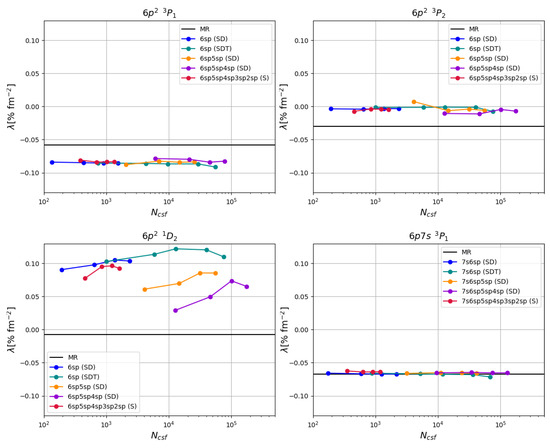
Figure 4.
The proportionality constant in the linear fit for the BR effect. Each data series corresponds to one set of active peel subshells and the four data points in each series correspond to one, …, four virtual layers. The horizontal black line in each plot indicates the value of calculated with only the multireference CSFs.
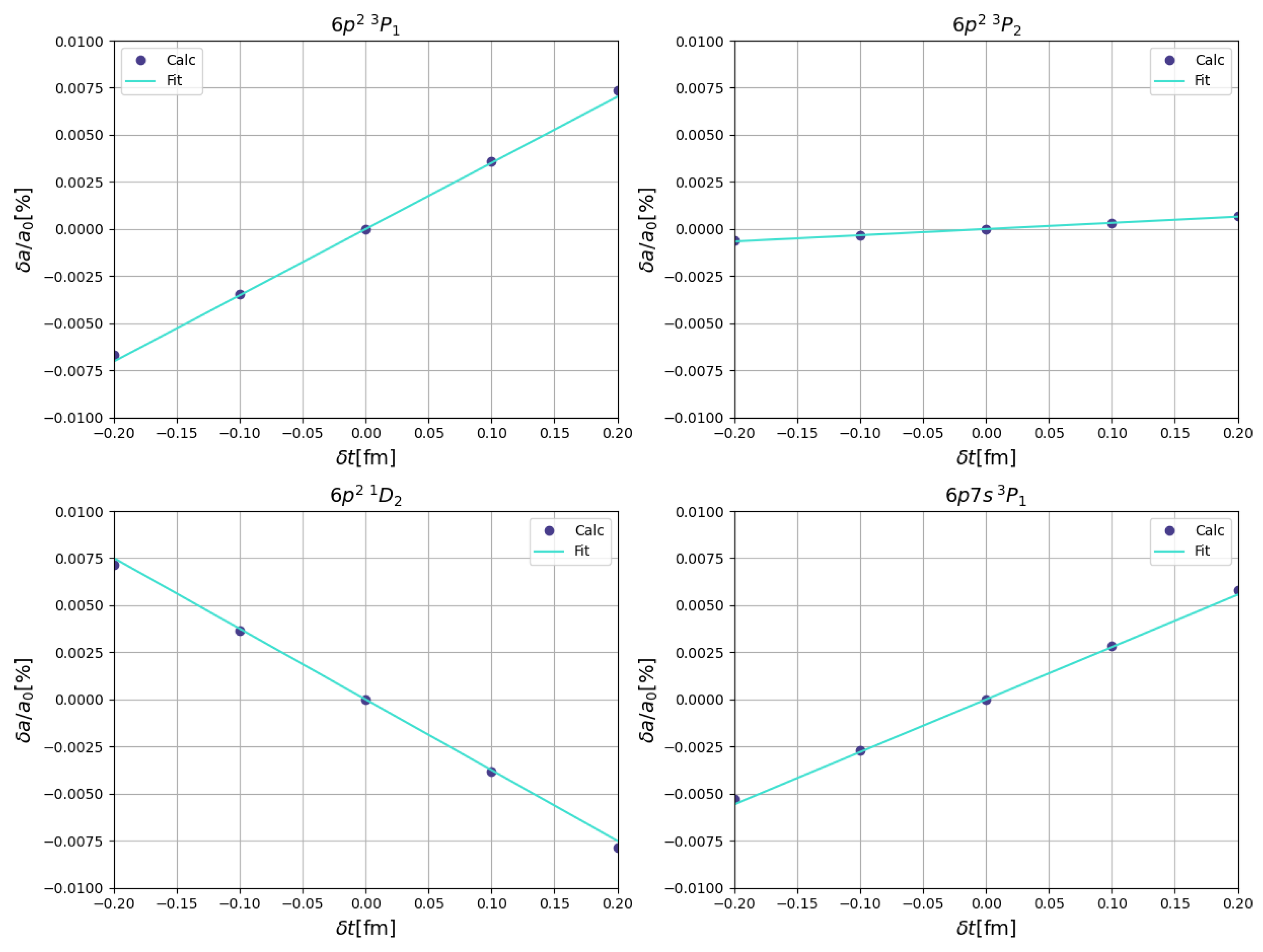
Variation in Skin Thickness
The effects of deformation can be investigated by studying the effect of a varying skin thickness t, that is, the diffuseness parameter b. The effect is expected to be small so the calculation was only performed for single excitations from to four virtual layers. In the calculations, the nuclear skin thickness varied by fm and fm from the default value fm. These deviations correspond to one and two standard deviations in the skin thickness obtained for nuclei with nucleon number by fitting to scattering data [19].
The relative change in the calculated hfs constant a is presented in Figure 5. The proportionality constant in the linear fit is used for the skin thickness. In units of , the values , , and were obtained, with corresponding coefficients of correlation for all states.

Figure 5.
Relative change in the hfs constant against variation in the skin thickness of the nuclear Fermi charge distribution from the reference nucleus with hfs constant , based on the expansion generated with S excitations from to four virtual layers. The straight line is the linear fit .
5. Discussion
5.1. Variation in Radius
Calculations of the proportionality constant for the BR effect were performed for 20 CSF expansions of various sizes. For the and states, the obtained values of were all in the , and , respectively. Including only the values calculated at the fourth virtual layer, these intervals are reduced to and in units of with no relative error of greater than ≈5% and ≈7%, respectively. This limitation is justified since all corresponding series of a-calculations in the 207Pb reference isotope achieved convergence towards the experimental value at the fourth virtual layer in both and . In addition, the expansion including valence-only correlations, gave values at the lower part of the interval while expansions adding core correlations yielded values in the upper part. Since the latter expansions could more accurately reproduce the experimental value of a, it was deemed sensible to recommend values slightly toward the higher end of the intervals as the more probable -values. That is, and are recommended. The uncertainties are given as about twice the range of the -values.
In it was found that the BR effect is practically non-existent, with a tendency for a small negative value. The calculated values of in units of range in the interval . Since this state did not converge toward the experimental a in the 207Pb reference isotope as the active set was increased, it is questionable to put more weight on the fourth virtual layer. Since all the expansions underestimated a, and a clear trend with an undershoot of a was observed, the higher the corresponding value of . To limit the number of calculated -values based on different expansions only those yielding a calculated a within of the experimental value are used. This reduces the interval to , as only three expansions achieved this accuracy (SD excitations from to one, two and four virtual layers, respectively). It should be noted that the series corresponding to SD excitations from and S excitations from approached the experimental a-value, although not reaching the accuracy limit. The corresponding -values also converged towards a similar range. Thus, the value is recommended. The uncertainty is chosen as twice the interval in question. This is a remarkably low value and similar to the finding in the state in potassium [21]. The explanation for this is not known and should be investigated in detail. It may indicate that the hyperfine anomaly due to the BR- and BW-effect is almost zero in since their behaviour is very similar.
In the final state, , all obtained values of were , with the greatest value being over four times the smallest. It should be noted that takes the opposite sign, compared to expectations. These were also the most scattered results obtained, including considerable deviation in within each series. This is in accord with being the state with the greatest range of calculated a-values in 207Pb. One should notice that only five of the 20 obtained -values were based on expansions that yielded a calculated a within of the experimental value. By using these five, the interval reduces to . If only those within of the experimental are included, further reducing interval to , with only two expansions. In the series including cv and cc correlation, there is some indication of convergence towards a value in the same range, but these results are inconclusive. It might be important to perform more comprehensive calculations adding further virtual layers may be performed to see if the calculated -values converge. Due to these facts, the value is recommended as the uncertainty may be large.
5.2. Expansions
From the calculations using different expansions, it is clear that the sensitivity varies. In the case of the and states the -values hardly change, even if the state differs from the multireference CSF. While the and states are more sensitive, even if the values show tendencies to converge. How well the calculated a-values compare to the experimental values seems to be a good indicator of the validity of the -value. This indicates that basing calculations of the BR-correction on an ASF that accurately reproduces the experimentally obtained value of the hfs constant a is important. This is especially important in , where the vast range of obtained -values dramatically reduced when removing expansions corresponding to inaccurate a-values. Moreover, and has the most consistent calculated a-values near the experimental value in the 207Pb isotope, and also the most consistent calculated . The same behaviour is seen within the different series: where there were larger changes in the calculated a, also gives larger changes in the calculated .
5.3. Comparisons with Other Calculations
The results of the systematic study by Rosenberg and Stroke [9] can not be directly compared to our results as they calculated the s- and electron contributions to the BR-effect between isotope-pairs, not taking mixing of other electrons into account. Extrapolating their values to Pb gives the same order of magnitude, for the and states. Gustavsson and Mårtensson-Pendrill [22] reported values in Tl (Z = 81) of and for the and electrons, respectively. While Heggset and Persson [11] found and in the configuration in Hg. The values are in the same order as our results indicating that our results are reasonable.
5.4. hfa in Pb and BR-Anomaly
The calculated -values in combination with nuclear charge radii gives the BR-anomaly which can be compared with experimental hfa. This will give an indication of how important a correction due to the BR-anomaly can be. In the case of Pb, the hyperfine anomaly is only known in four isotopes [3,18] as shown in Table 5 with compared to for the reference isotope . Since the BR-effect is only expected to be of major importance when the BW-effect is small, that is when the spins of the nuclei are the same [2,3], we observe that the BR-correction is negligible relative to .
Table 5.
Experimental hyperfine anomaly in Pb isotopes and calculated BR-correction.
The values of and errors when taking the hfa between the isotopes are much larger than the value of the BR-correction, why it is safe to assume that the BR-effect can be neglected in Pb until experiments on the hfs with higher accuracy are performed.
6. Conclusions
The differential Breit-Rosenthal effect for the , and states in Pb has been calculated. The recommended values are given in Table 6. Our investigation indicates that the quality of the value of the differential Breit-Rosenthal effect is related to how well the calculation of the a-factor correlates with the experimental value which indicates that it might not be sufficient to perform calculations with small expansions if the experimental a-factor is not well reproduced, but the size of the expansions must be adapted for the specific situation. It is found that the accuracy of the experimental values of the hfa in Pb does not allow for a comparison with the calculations, but it seems like the BR-effect can be neglected.
Table 6.
Recommended values of the differential Breit-Rosenthal effect.
Author Contributions
Conceptualization, J.R.P.; methodology, M.K.K. and J.R.P.; software, M.K.K.; validation, J.R.P.; formal analysis, M.K.K. and J.R.P.; investigation, M.K.K. and J.R.P.; data curation, M.K.K. and J.R.P.; writing—original draft preparation, M.K.K. and J.R.P.; writing—review and editing, M.K.K. and J.R.P.; visualization, M.K.K.; supervision, J.R.P.; project administration, J.R.P. All authors have read and agreed to the published version of the manuscript.
Funding
This research received no external funding.
Data Availability Statement
The data presented in this study are available on request from the corresponding author. The data are not publicly available due to legal reasons.
Conflicts of Interest
The authors declare no conflict of interest.
References
- Otten, E.W. Nuclear radii and moments of unstable isotopes. In Treatise on Heavy Ion Science; Springer: Berlin/Heidelberg, Germany, 1989; pp. 517–638. [Google Scholar]
- Büttgenbach, S. Magnetic Hyperfine Anomalies. Hyperfine Interact. 1984, 20, 1–64. [Google Scholar] [CrossRef]
- Persson, J. Table of hyperfine anomaly in atomic systems—2023. At. Data Nucl. Data Tables 2023, 154, 101589. [Google Scholar] [CrossRef]
- Bohr, A.; Weisskopf, V. The influence of nuclear structure on the hyperfine structure of heavy elements. Phys. Rev. 1950, 77, 94. [Google Scholar] [CrossRef]
- Fujita, T.; Arima, A. Magnetic hyperfine structure of muonic and electronic atoms. Nucl. Phys. A 1975, 254, 513–541. [Google Scholar] [CrossRef]
- Rosenthal, J.E.; Breit, G. The isotope shift in hyperfine structure. Phys. Rev. 1932, 41, 459. [Google Scholar] [CrossRef]
- Crawford, M.; Schawlow, A. Electron-nuclear potential fields from hyperfine structure. Phys. Rev. 1949, 76, 1310. [Google Scholar] [CrossRef]
- Ionesco-Pallas, N. Nuclear Magnetic Moments from Hyperfine Structure Data. Phys. Rev. 1960, 117, 505. [Google Scholar] [CrossRef]
- Rosenberg, H.; Stroke, H. Effect of a diffuse nuclear charge distribution on the hyperfine-structure interaction. Phys. Rev. A 1972, 5, 1992. [Google Scholar] [CrossRef]
- Angeli, I.; Marinova, K.P. Table of experimental nuclear ground state charge radii: An update. At. Data Nucl. Data Tables 2013, 99, 69–95. [Google Scholar] [CrossRef]
- Heggset, T.; Persson, J.R. Calculation of the Differential Breit–Rosenthal Effect in the 6s6p 3P1,2, States of Hg. Atoms 2020, 8, 86. [Google Scholar] [CrossRef]
- Fischer, C.F.; Gaigalas, G.; Jönsson, P.; Bieron, J. GRASP2018—A Fortran 95 version of the general relativistic atomic structure package. Comput. Phys. Commun. 2019, 237, 184–187. [Google Scholar] [CrossRef]
- Fischer, C.F.; Godefroid, M.; Brage, T.; Jönsson, P.; Gaigalas, G. Advanced multiconfiguration methods for complex atoms: I. Energies and wave functions. J. Phys. B At. Mol. Opt. Phys. 2016, 49, 182004. [Google Scholar] [CrossRef]
- Grant, I.P. Relativistic Quantum Theory of Atoms and Molecules: Theory and Computation; Springer Science & Business Media: Berlin/Heidelberg, Germany, 2007; Volume 40. [Google Scholar]
- Bieroń, J.; Froese Fischer, C.; Gaigalas, G.; Grant, I.P.; Jönsson, P. A Practical Guide to GRASP2018—A Collection of Fortran 95 Programs with Parallel Computing Using MPI; Technical Report; Computational Atomic Structure Group: San Francisco, CA, USA, 2018. [Google Scholar]
- Karlsen, M.K. Calculation of the Breit-Rosenthal Effect in Pb I. Master’s Thesis, NTNU, Trondheim, Norway, 2023. [Google Scholar]
- Stone, N. Table of nuclear magnetic dipole and electric quadrupole moments. At. Data Nucl. Data Tables 2005, 90, 75–176. [Google Scholar] [CrossRef]
- Persson, J. Hyperfine structure and hyperfine anomaly in Pb. J. Phys. Commun. 2018, 2, 055028. [Google Scholar] [CrossRef]
- Elton, L.R.B. Nuclear Sizes; Oxford University Press: London, UK, 1961; Volume 561. [Google Scholar]
- Froese-Fischer, C.; Brage, T.; Johnsson, P. Computational Atomic Structure: An MCHF Approach; CRC Press: Boca Raton, FL, USA, 1997. [Google Scholar]
- Demidov, Y.A.; Kozlov, M.G.; Barzakh, A.E.; Yerokhin, V.A. Bohr-Weisskopf effect in the potassium isotopes. Phys. Rev. C 2023, 107, 024307. [Google Scholar] [CrossRef]
- Gustavsson, M.G.; Mårtensson-Pendrill, A.M. Four decades of hyperfine anomalies. In Advances in Quantum Chemistry; Elsevier: Amsterdam, The Netherlands, 1998; Volume 30, pp. 343–360. [Google Scholar]
Disclaimer/Publisher’s Note: The statements, opinions and data contained in all publications are solely those of the individual author(s) and contributor(s) and not of MDPI and/or the editor(s). MDPI and/or the editor(s) disclaim responsibility for any injury to people or property resulting from any ideas, methods, instructions or products referred to in the content. |
© 2024 by the authors. Licensee MDPI, Basel, Switzerland. This article is an open access article distributed under the terms and conditions of the Creative Commons Attribution (CC BY) license (https://creativecommons.org/licenses/by/4.0/).