Stark Broadening of Lyman-α in the Presence of a Strong Magnetic Field

Abstract

Stark broadening of Lyman-$\alpha$ of a hydrogen-like atom in the presence of a strong magnetic field is analyzed. The shape of the central ($\pi$) component of the Lorentz–Zeeman triplet is expressed analytically, taking into account the plasma coupling and microfield dynamic effects. It is shown that in a sufficiently strong magnetic field, the broadening of this component, contrary to the broadening of the lateral ($\sigma$) ones, is independent of the magnetic field and, therefore, can be used for the plasma density diagnostics. Comparison with computer simulations at conditions typical for tokamak divertors and white dwarf atmospheres shows a very good agreement.

1. Introduction

Hydrogen atom is the simplest and best understood atomic system. It was the first real physical object to which the quantum mechanical description—first of the “old” Bohr’s theory [1], then the modern quantum mechanics [2]—was applied and tested against.

The simplest transition in hydrogen or a hydrogen-like ion is Lyman-$\alpha$ ($n=2\to n=1$, where n is the principal quantum number). Nevertheless, this transition represents a challenge for some models of plasma line broadening [3]. The reason is a strong influence of the ion dynamic effect, and in particular the directionality of the ion microfields [4] on the shape of the central Stark component of this line. Because of this effect, the Stark broadening of Lyman-$\alpha$ changes from the impact broadening [5] in the high-temperature/low-density regime to the so-called rotation broadening [6] in a low-temperature/high-density plasma, in a stark contrast to the majority of spectral lines that converge to the quasistatic lineshape [5].

In the presence of a sufficiently strong magnetic field, Lyman-$\alpha$ assumes a familiar Zeeman triplet pattern. However, its central ($\pi$, $\Delta M=0$) and lateral (${\sigma }^{\pm }$, $\Delta M=\pm 1$) components are broadened by the plasma Stark effect differently: Due to the degeneracy removal by the applied magnetic field, the upper states of the $\sigma$ components, $\left|2p\pm 1\right.⟩$, are subject to the quadratic Stark effect, while that of the $\pi$ component, $\left|2p0\right.⟩$, remains degenerate with $\left|2s0\right.⟩$ and, therefore, linearly depends on the electric field. As a result, the lateral components become significantly narrower than the central one [7].

2. Analytical Model

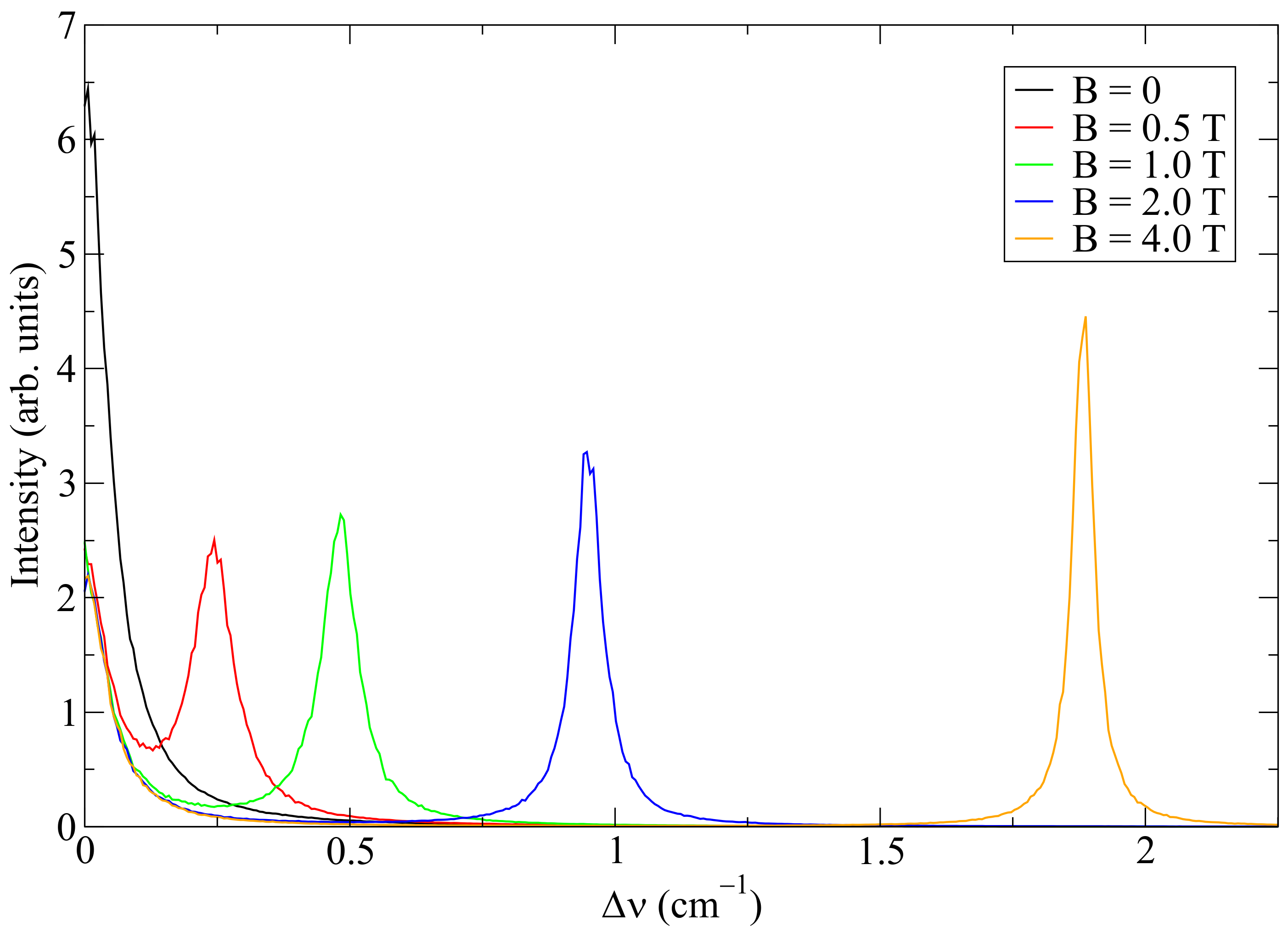
As an example, let us assume plasma conditions relevant to tokamak divertors. Specifically, the electron and ion temperature $T_e=T_i=1eV$, the electron density $n_e={10}^{14}{\mathrm{cm}}^{-3}$, and the magnetic field B on the order of 1 T. A comparison of plasma-broadened Lyman-$\alpha$ shapes in the presence of the magnetic field is given in Figure 1 (see Section 3 for the details of these calculations). It is seen that for a non-zero magnetic field, the widths of the $\pi$ and $\sigma$ components of the Zeeman triplet are different, in agreement with the earlier findings [7]. Notably, as the magnetic-field strength increases, the Stark broadening of the central component remains nearly constant, whereas the lateral components become narrower.

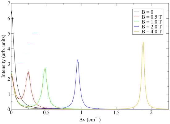
Figure 1. Stark-broadened Lyman-$\alpha$ shapes assuming $n_e={10}^{14}{\mathrm{cm}}^{-3}$, $T=1\mathrm{eV}$, and a few values of the magnetic field as indicated in the legend.

To understand this result, consider Hamiltonian of the $n=2$ manifold under the crossed $\overrightarrow{F}$ and $\overrightarrow{B}$ fields, e.g., see [8]:

$$V_2=\left(\begin{array}{cccc}0& 0& f& 0\\ 0& -bcos\theta & {\displaystyle \frac{b}{\sqrt{2}}}sin\theta & 0\\ f& {\displaystyle \frac{b}{\sqrt{2}}}sin\theta & 0& {\displaystyle \frac{b}{\sqrt{2}}}sin\theta \\ 0& 0& {\displaystyle \frac{b}{\sqrt{2}}}sin\theta & bcos\theta \end{array}\right),$$

(1)

where for compactness $f:={\displaystyle \frac{3}{Z}}F$ and $b:={\displaystyle \frac{\alpha }{2}}B$ definitions are used, $\theta$ is the angle between $\overrightarrow{F}$ and $\overrightarrow{B}$, and $\overrightarrow{F}$ is assumed to lie along the quantization axis. Here, the spin degree of freedom is ignored (i.e., the magnetic-field perturbation is assumed to be much stronger than the fine structure). The atomic units ($ħ=e=m_e=1$) are used, $\alpha$ is the fine-structure constant, and Z is the charge of the nucleus ($Z=1$ in the case of hydrogen).

The eigenvalues of $V_2$ are

$${(\Delta E)}^2=\frac{b^2+f^2}{2}\pm \sqrt{{\left(\frac{b^2+f^2}{2}\right)}^2-f^2{b}^2{cos}^2\theta }.$$

(2)

In the strong-B limit, i.e., $b\gg f$, this expression reduces to

$$\Delta E_{\pi }=\pm fcos\theta$$

(3)

and

$$\Delta E_{\sigma }=\pm (b+\frac{f^2}{2b}{sin}^2\theta )$$

(4)

for the $\pi$ and $\sigma$ components, respectively. Thus, the Stark effect of the central component is linear (it is split into two sub-components), on the order of f, and independent of b, while that of the lateral components is quadratic, narrow ($\ll f$), and inversely proportional to b. The intensities of all four components, up to the $\mathcal{O}\left({(f/b)}^2\right)$ terms, depend neither on the field magnitudes nor on the angle between the fields and are equal to 1/3 (${\sigma }^{\pm }$) and 1/6 (each of the split-$\pi$ sub-components) of that of the unperturbed Lyman-$\alpha$ line.

The total area-normalized line shape $L\left(\omega \right)$ is a sum of the $\pi$ and $\sigma$ components which, after averaging over $\theta$ (but keeping f fixed) become, respectively,

$$L_{\pi }\left(\omega \right)=\left\{\begin{array}{cc}{\displaystyle \frac{1}{6f}},\hfill & \left|\omega \right|\le f\hfill \\ 0,\hfill & \mathrm{elsewhere}\hfill \end{array}\right.$$

(5)

and

$$L_{\sigma }\left(\omega \right)=\left\{\begin{array}{cc}{\displaystyle \frac{b}{3f\sqrt{f^2-2b\left(\right|\omega |-b)}}},\hfill & b\le \left|\omega \right|<b+{\displaystyle \frac{f^2}{2b}}\hfill \\ 0,\hfill & \mathrm{elsewhere}.\hfill \end{array}\right.$$

(6)

From Equation (5) it follows that $L_{\pi }\left(\omega \right)$ assumes a rectangular shape—a result recently obtained by [9]. Notably, this is the shape of any high-n H-like transition in the quasi-contiguous (QC) approximation [10]. Therefore, one can directly apply the QC-FFM approach [11] to obtain the $\pi$ lineshape accounting for the microfield dynamics through the frequency-fluctuation model (FFM) [12,13]. Assuming the dynamic broadening of each of the $\pi$ and ${\sigma }^{\pm }$ components is independent [14], for a one-component plasma (OCP) one obtains

$$L_{\pi }(\overline{\nu };\overline{\omega })=\frac{1}{\pi }\Re \frac{J(\overline{\nu };\overline{\omega })}{1-\overline{\nu }J(\overline{\nu };\overline{\omega })},$$

(7)

where ℜ stands for the real part and

$$J(\overline{\nu };\overline{\omega })={\int }_0^{\infty }\mathrm{d}\tau exp[-\varphi \left(\tau \right)-i(\overline{\omega }-i\overline{\nu })\tau ].$$

(8)

Here, the line shape is expressed as a function of the dimensionless reduced detuning $\overline{\omega }=\omega /{\Delta }_0$ and $\overline{\nu }$—a single parameter related to the typical frequency of the microfields in the radiator–perturber center-of-mass frame [15]

$$w_{\mathrm{dyn}}=\sqrt{\frac{k{T}_p}{m_p}+\frac{k{T}_r}{m_r}}{\left(\frac{4\pi n_p}{3}\right)}^{1/3}$$

(9)

via

$$\overline{\nu }=\frac{1}{2}\frac{w_{\mathrm{dyn}}}{{\Delta }_0}+\frac{1}{20}{\left(\frac{w_{\mathrm{dyn}}}{{\Delta }_0}\right)}^2,$$

(10)

where the second term is a semiempirical correction to recover the impact limit [5]. $Z_p$, $n_p$, $m_p$, and $T_p$ are the charge, density, mass, and temperature of the OCP particles; $m_r$ and $T_r$ are the mass and temperature of the radiator. The normal detuning ${\Delta }_0$ in several expressions above is defined as

$${\Delta }_0=\frac{3}{Z}{F}_0,$$

(11)

where $F_0=2\pi {(4/15)}^{2/3}{Z}_p{n}_p^{2/3}$ is the Holtsmark normal field strength [16].

In Equation (8), $\varphi \left(\tau \right)$ is the characteristic function of the probability distribution of the plasma microfield magnitudes $\beta =F/F_0$

$$W\left(\beta \right)=\frac{2}{\pi }\beta {\int }_0^{\infty }xsin\left(\beta x\right)exp[-\varphi (x\left)\right]\mathrm{d}x.$$

(12)

For a neutral radiator, one can use [17]

$$\varphi \left(x\right)=x^{3/2}/(1+1.295\sqrt{{\Gamma }_{p}x}+0.606{\Gamma }_{p}x),$$

(13)

where ${\mathrm{\Gamma }}_p$ is the coupling parameter.

To summarize, Equations (7)–(13) allow for calculating the shape of the Lyman-$\alpha$$\pi$ component as broadened by a single plasma species (electrons or ions). The total line shape is obtained by a convolution of the individual contributions [18].

3. Computer Simulations

A variant of computer simulations (CS) described in Ref. [19] is used. Briefly, the Heisenberg equation

$$-i\frac{\partial }{\partial t}\overrightarrow{d}\left(t\right)=\left[H\left(t\right),\overrightarrow{d}\left(t\right)\right]$$

(14)

is numerically solved by introducing the time-development operator $\mathcal{U}\left(t\right)$ in the interaction representation,

$$i\frac{d\mathcal{U}\left(t\right)}{dt}={\widehat{V}}_I\left(t\right)\mathcal{U}\left(t\right)$$

(15)

with

$${\widehat{V}}_I\left(t\right)=e^{i{H}_{0}t}{V}_I\left(t\right)e^{-i{H}_{0}t}$$

(16)

The time evolution of the dipole operator is then given by

$$\overrightarrow{d}\left(t\right)={\mathcal{U}}^{†}\left(t\right)e^{i{H}_{0}t}\overrightarrow{d}{e}^{-i{H}_{0}t}\mathcal{U}\left(t\right)$$

(17)

with Fourier transform

$$\overrightarrow{d}\left(\omega \right)={\int }_0^{\infty }dt{e}^{i\omega t}\overrightarrow{d}\left(t\right).$$

(18)

Assuming the radiator density matrix is diagonal, which is customary in line shape broadening calculations [5], the line shape is

$$L\left(\omega \right)\propto \sum _{if}{\rho }_i⟨|{\overrightarrow{d}}_{fi}{\left(\omega \right)|}^2⟩,$$

(19)

where the sums are over initial and final states i and f, respectively, and the plasma average denoted by the angle brackets is accomplished by averaging over CS runs.

The motion of the plasma quasiparticles (both plasma electrons and ions) is described by the screened monopole interaction using a velocity Verlet algorithm [20]. However, for the present calculations, the radiators are neutral, therefore, the trajectories of all plasma particles were assumed to be straight.

Each ion species s is assigned a different screening length. For a weakly coupled plasma, the inverse screening length ${\kappa }_s$ includes screening by all other charged particles with the same or lesser mass,

$${\kappa }_s^2=\sum _{s^{\prime }(m_{s^{\prime }}\le m_s)}\frac{4\pi n_{s^{\prime }}{Z}_{s^{\prime }}^2}{k{T}_{s^{\prime }}},$$

(20)

with $m_s$, $n_s$, and $T_s$ the mass, number density, and temperature of species s in the plasma.

The simulation follows the reduced-mass model [21] with a fixed, static radiator at the center of a spherical box of radius several times the electron Debye length to ensure convergence [22]. Whenever a perturber exits the simulation volume, it is reinjected at a random point on the sphere surface with a velocity randomly chosen according to the 2D Gaussian distribution in the tangential plane and Rayleigh distribution in the radial direction.

4. Results and Conclusions

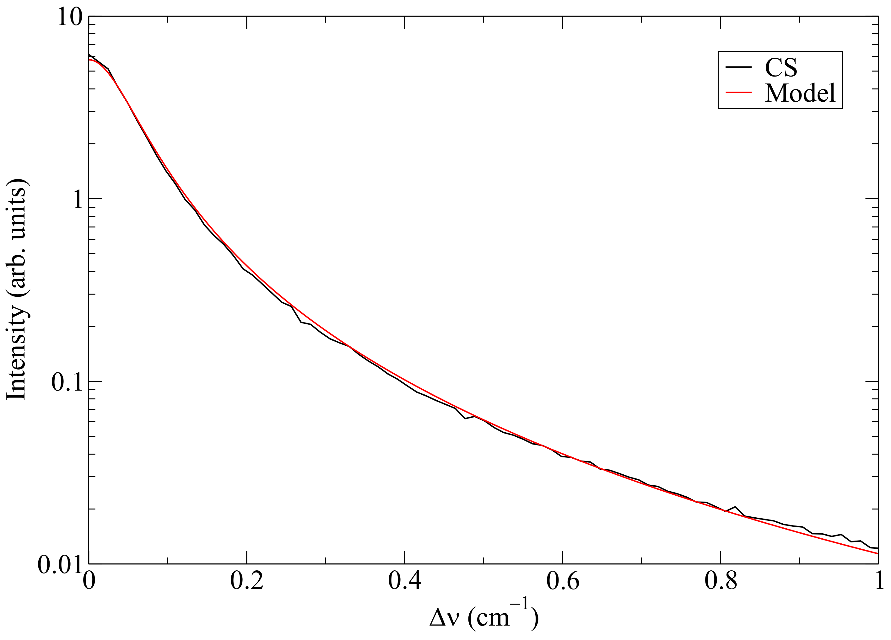
In Figure 2, a comparison between the Lyman-$\alpha$$\pi$ line shapes calculated by the analytical model (Section 2) and computer simulations (Section 3) is shown, indicating a good agreement between the two.

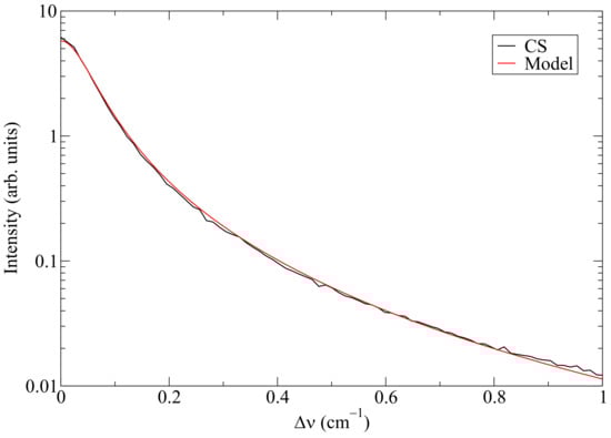
Figure 2. Comparison of the Lyman-$\alpha$$\pi$ line shape calculated using the computer simulations (CS) and the analytical model. $n_e={10}^{14}{\mathrm{cm}}^{-3}$, $T=1\mathrm{eV}$, and $B=4T$.

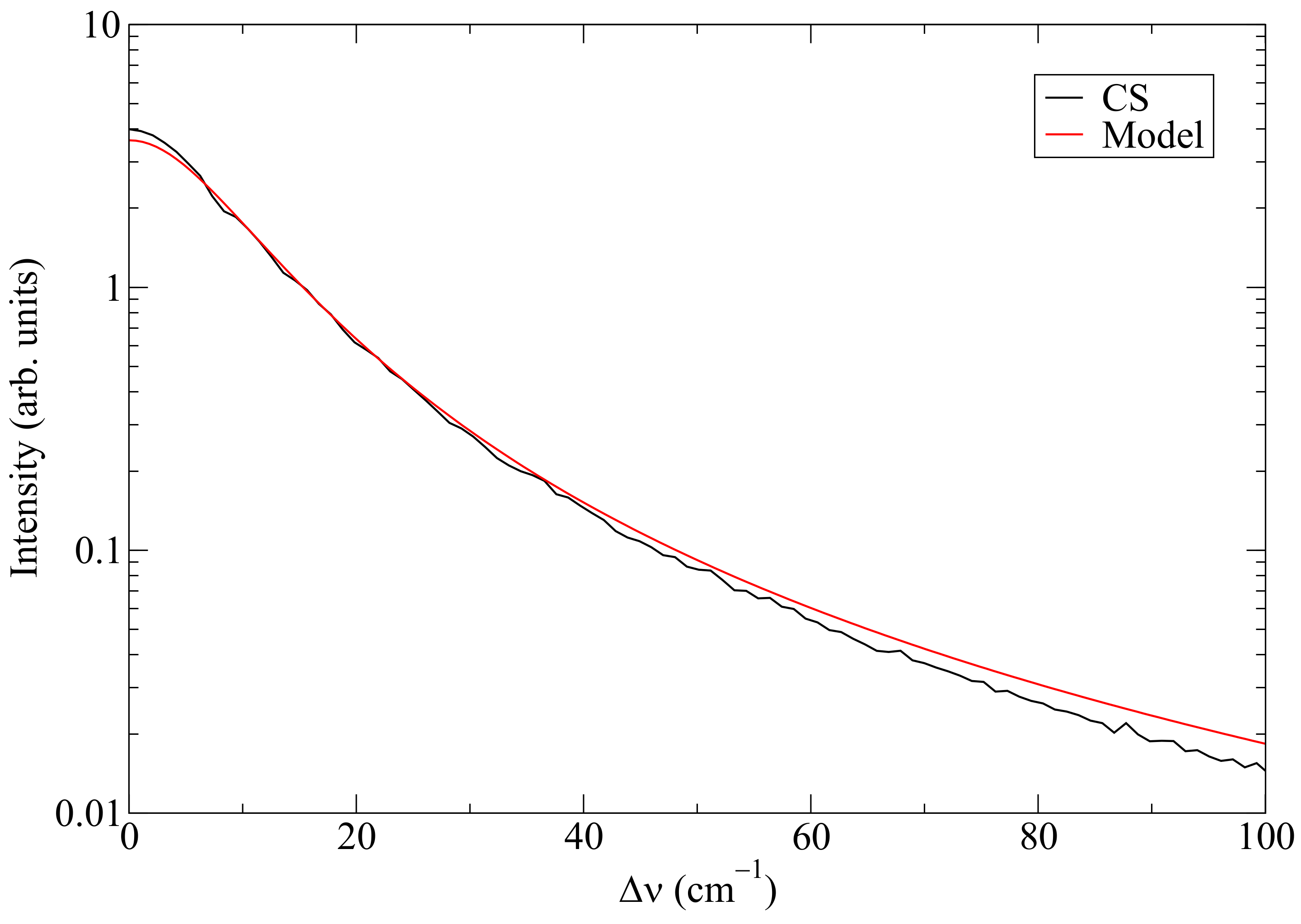
In white dwarf atmospheres, the magnetic field can easily reach hundreds of teslas, e.g., see [23], with the electron density about ${10}^{17}{\mathrm{cm}}^{-3}$ to ${10}^{18}{\mathrm{cm}}^{-3}$ [24]. In Figure 3, a comparison under such conditions is shown. As in the previous example, a good agreement is seen. In both examples, the values of the full width at half maximum (FWHM) of the lineshapes differ by ∼15%.

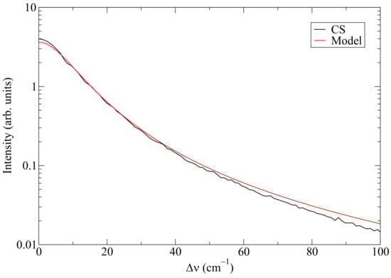
Figure 3. Same as Figure 2, but for $n_e={10}^{17}{\mathrm{cm}}^{-3}$, $T=1\mathrm{eV}$, and $B=400T$.

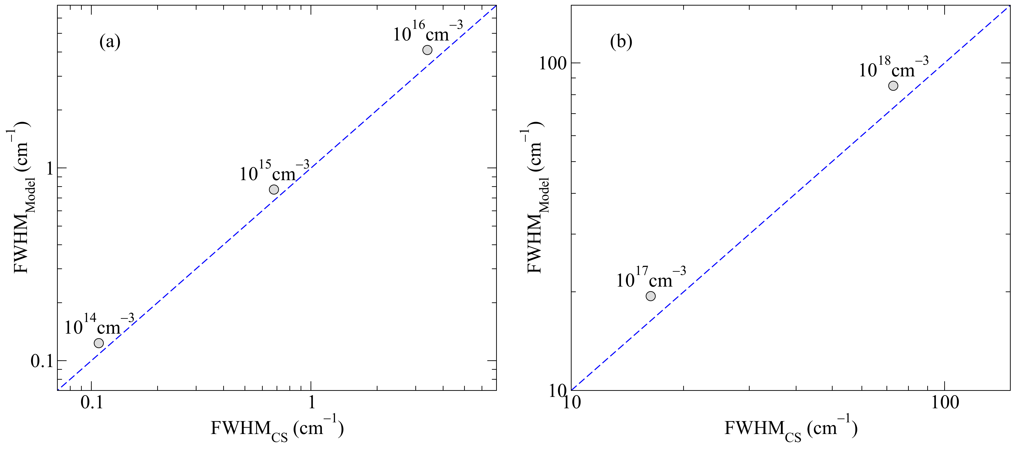
Notably, this value (∼15%) of the extraneous width predicted by the model remains almost constant over a very wide range of the plasma densities, as shown in Figure 4. Thus, for practical purposes, it may be suggested to multiply the width given by the model by the 0.85 factor. It is also noted that the model remains sufficiently accurate even beyond its domain of applicability ($b\gg f$): indeed, at $n_e={10}^{16}c{m}^{-3}$ (the last datum in Figure 4a), $b\approx f$; however, the disagreement between the simulations and the model is about 20% or, using the corrective 0.85 factor, only 5%.

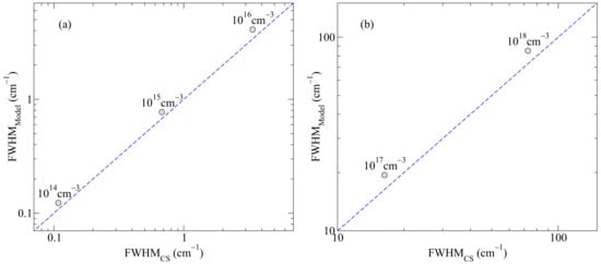
Figure 4. Comparison of the Lyman-$\alpha$$\pi$ broadening as given by the computer simulations and the model over wide ranges of densities. $B=4T$ (a) and $B=400T$ (b) are assumed.

To conclude, in this study it is demonstrated that in the strong-B limit, when the three components of the Lyman-$\alpha$ Zeeman triplet are well-resolved, the broadening of the central, $\pi$ component is independent of the magnetic field and, thus, can be used for the plasma density diagnostics, as has recently been suggested [9]. Furthermore, the shape of this component is expressed analytically.

References

- Bohr, N.I. On the constitution of atoms and molecules. Lond. Edinburgh Dublin Philos. Mag. J. Sci. 1913, 26, 1–25. [Google Scholar] [CrossRef]
- Schrödinger, E. Quantisierung als Eigenwertproblem. Annalen Physik 1926, 384, 361–376. [Google Scholar] [CrossRef]
- Stambulchik, E. Review of the 1st Spectral Line Shapes in Plasmas code comparison workshop. High Energy Density Phys. 2013, 9, 528–534. [Google Scholar] [CrossRef]
- Calisti, A.; Demura, A.; Gigosos, M.A.; González-Herrero, D.; Iglesias, C.A.; Lisitsa, V.S.; Stambulchik, E. Influence of microfield directionality on line shapes. Atoms 2014, 2, 259–276. [Google Scholar] [CrossRef]
- Griem, H.R. Spectral Line Broadening by Plasmas; Academic: New York, NY, USA, 1974. [Google Scholar]
- Stambulchik, E.; Demura, A.V. Dynamic Stark broadening of Lyman-α. J. Phys. B At. Mol. Opt. Phys. 2016, 49, 035701. [Google Scholar] [CrossRef]
- Rosato, J.; Marandet, Y.; Capes, H.; Ferri, S.; Mosse, C.; Godbert-Mouret, L.; Koubiti, M.; Stamm, R. Stark broadening of hydrogen lines in low-density magnetized plasmas. Phys. Rev. E 2009, 79, 046408-7. [Google Scholar] [CrossRef]
- Stambulchik, E.; Maron, Y. Zeeman effect induced by intense laser light. Phys. Rev. Lett. 2014, 113, 083002. [Google Scholar] [CrossRef]
- Oks, E. Analytical results for the Stark–Zeeman broadening of the Lyman-alpha line in plasmas. Int. Rev. At. Mol. Phys. 2023, 14, 43–48. [Google Scholar] [CrossRef]
- Stambulchik, E.; Maron, Y. Stark effect of high-n hydrogen-like transitions: Quasi-contiguous approximation. J. Phys. B At. Mol. Opt. Phys. 2008, 41, 095703. [Google Scholar] [CrossRef]
- Stambulchik, E.; Maron, Y. Quasicontiguous frequency-fluctuation model for calculation of hydrogen and hydrogenlike Stark-broadened line shapes in plasmas. Phys. Rev. E 2013, 87, 053108. [Google Scholar] [CrossRef]
- Calisti, A.; Mossé, C.; Ferri, S.; Talin, B.; Rosmej, F.; Bureyeva, L.A.; Lisitsa, V.S. Dynamic Stark broadening as the Dicke narrowing effect. Phys. Rev. E 2010, 81, 016406. [Google Scholar] [CrossRef]
- Bureeva, L.A.; Kadomtsev, M.B.; Levashova, M.G.; Lisitsa, V.S.; Calisti, A.; Talin, B.; Rosmej, F. Equivalence of the method of the kinetic equation and the fluctuating-frequency method in the theory of the broadening of spectral lines. JETP Lett. 2010, 90, 647–650. [Google Scholar] [CrossRef]
- Ferri, S.; Calisti, A.; Mossé, C.; Mouret, L.; Talin, B.; Gigosos, M.A.; González, M.A.; Lisitsa, V. Frequency-fluctuation model applied to Stark-Zeeman spectral line shapes in plasmas. Phys. Rev. E 2011, 84, 026407. [Google Scholar] [CrossRef] [PubMed]
- Stambulchik, E.; Maron, Y. Plasma Formulary Interactive. J. Instrum. 2011, 6, P10009. [Google Scholar] [CrossRef]
- Holtsmark, J. Über die Verbreiterung von Spektrallinien. Ann. Phys. 1919, 363, 577–630. [Google Scholar] [CrossRef]
- Dzierżęga, K.; Sobczuk, F.; Stambulchik, E.; Pokrzywka, B. Studies of spectral line merging in a laser-induced hydrogen plasma diagnosed with two-color Thomson scattering. Phys. Rev. E 2021, 103, 063207. [Google Scholar] [CrossRef]
- Mossé, C.; Calisti, A.; Ferri, S.; Talin, B.; Bureyeva, L.A.; Lisitsa, V.S. Universal FFM hydrogen spectral line shapes applied to ions and electrons. AIP Conf. Proc. 2008, 1058, 63–65. [Google Scholar] [CrossRef]
- Stambulchik, E.; Maron, Y. A study of ion-dynamics and correlation effects for spectral line broadening in plasma: K-shell lines. J. Quant. Spectrosc. Radiat. Transfer 2006, 99, 730–749. [Google Scholar] [CrossRef]
- Verlet, L. Computer “Experiments” on Classical Fluids. I. Thermodynamical Properties of Lennard-Jones Molecules. Phys. Rev. 1967, 159, 98–103. [Google Scholar] [CrossRef]
- Seidel, J.; Stamm, R. Effects of radiator motion on plasma-broadened hydrogen Lyman-β. J. Quant. Spectrosc. Radiat. Transfer 1982, 27, 499–503. [Google Scholar] [CrossRef]
- Rosato, J.; Capes, H.; Stamm, R. Ideal Coulomb plasma approximation in line shape models: Problematic issues. Atoms 2014, 2, 253–258. [Google Scholar] [CrossRef]
- Raji, A.; Rosato, J.; Stamm, R.; Marandet, Y. New analysis of Balmer line shapes in magnetic white dwarf atmospheres. Eur. Phys. J. D 2021, 75, 63. [Google Scholar] [CrossRef]
- Falcon, R.E.; Rochau, G.A.; Bailey, J.E.; Gomez, T.A.; Montgomery, M.H.; Winget, D.E.; Nagayama, T. Laboratory measurements of white dwarf photospheric spectral lines: Hβ. Astrophys. J. 2015, 806, 214. [Google Scholar] [CrossRef]
Disclaimer/Publisher’s Note: The statements, opinions and data contained in all publications are solely those of the individual author(s) and contributor(s) and not of MDPI and/or the editor(s). MDPI and/or the editor(s) disclaim responsibility for any injury to people or property resulting from any ideas, methods, instructions or products referred to in the content. |
© 2023 by the author. Licensee MDPI, Basel, Switzerland. This article is an open access article distributed under the terms and conditions of the Creative Commons Attribution (CC BY) license (https://creativecommons.org/licenses/by/4.0/).