Abstract
In the framework of the study of helium-like atomic systems possessing the collinear configuration, we propose a simple method for computing compact but very accurate wave functions describing the relevant S-state. It is worth noting that the considered states include the well-known states of the electron–nucleus and electron–electron coalescences as a particular case. The simplicity and compactness imply that the considered wave functions represent linear combinations of a few single exponentials. We have calculated such model wave functions for the ground state of helium and the two-electron ions with nucleus charge . The parameters and the accompanying characteristics of these functions are presented in tables for number of exponential from 3 to 6. The accuracy of the resulting wave functions are confirmed graphically. The specific properties of the relevant codes by Wolfram Mathematica are discussed. An example of application of the compact wave functions under consideration is reported.
1. Introduction
In this paper, we present a technique for building compact and simple wave functions of high accuracy, describing two-electron atomic systems such as H, He, Li, Be and B with the collinear arrangement of the particles [1]. The study of mechanism of double photoionization of the helium-like atomic systems by high energy photons [2,3] can serve as an example of possible application (see the details in the next Section).
Methods enabling us to calculate the relevant wave function (WF) and the corresponding non-relativistic energy differ from each other by the calculation technique, spatial variables and basis sets. It is well-known that the S-state WF, , is a function of three variables: the distances and between the nucleus and electrons, and the interelectron distance , where and represent radius-vectors of the electrons. We shall pay special attention to the bases that differ from each other both in the kind of the basis functions and in its number (basis size). The Hartree atomic units are used throughout the paper.
It would be useful to give some examples of basis sets intended for describing the relevant S states. The correlation function hyperspherical harmonic method (CFHHM) [4,5] employs the basis representing the product of the hyperspherical harmonic (HH) as an angular part, and the numerical radial part. The corresponding basis size N equals (as a rule) 625. The Pekeris-like method (PLM) [6,7,8] is used intensively in the current work. The basis size of the PLM under consideration is (for the number of shells ), and the basis functions can be finally reduced to the form , where and are the real constants and are non-negative integers. Hylleraas [9] (see also [10,11]) was the first who employed the same basis but with . The authors of Ref. [12] have performed variational calculations on the helium isoelectronic sequence using modification of the basis set that employed by Frankowski and Pekeris [13]. They managed to get very accurate results using the reduced basis of the size . The variational basis functions of the type with complex exponents were used in the works of Korobov [14] (–2200) and Frolov [15] for –2700 (see also references therein). Application of the Gaussian bases of the size can be found in the book [16]. The reviews on the helium-like atomic system and the methods of their calculations can be found, e.g., in the handbook [17].
In this paper, we propose a simple method of calculation of the compact but very accurate WFs describing the two-electron atom/ion with collinear configuration. The results and example of application of the relevant technique are presented in the next sections.
2. Calculation Technique
The simplicity of the WFs under consideration implies that the form
represents the sum of a few single exponentials, whereas the compactness means that their number in Equation (1), unlike the basis sizes mentioned in the introduction. The relevant accuracy will be discussed later. It is seen that the RHS of Equation (1) includes N linear parameters and N nonlinear parameters with .
The collinear arrangement of the particles consisting of the nucleus and two electrons can be described by a single scalar parameter as follows [1]:
where , and r is the distance between the nucleus and the electron most distant from it. Clearly corresponds to the electron–nucleus coalescence, and to the electron–electron coalescence. The boundary value corresponds to the collinear e-n-e configuration with the same distances of both electrons from the nucleus. In general, corresponds to the collinear arrangement of the form n-e-e where both electrons are on the same side of the nucleus. Accordingly, corresponds to the collinear arrangement of the form e-n-e where the electrons are on the opposite sides of the nucleus. The absolute value measures the ratio of the distances of the electrons from the nucleus.
Thus, for the particles with collinear arrangement we can introduce the collinear WF of the form
It should be emphasized that, e.g., the PLM WF with collinear configuration reduces to the form
where for the current (standard) consideration, as it was mentioned earlier.
We can give an example of the physical problem where the collinear WF of the form (4) cannot be applied, but the quite accurate WF of the form (1) is required instead. In Refs. [2,3], the mechanism of photoionization in the two-electron atoms is investigated. Calculations of various differential characteristics (cross sections) of ionization are based on computation of the triple integral of the form
where () are the momenta of photoelectrons, is the recoil momentum, , i is the imaginary unit, and is the confluent hypergeometric function of the first kind. The most important for our consideration is the fact that integral (5) contains the collinear WF describing the case of the electron–electron coalescence () in the helium-like atom/ion with the nucleus charge Z. It is clear that the numerical computation of the triple integral (5) is not impossible, but rather a difficult problem, especially for building the relevant graphs. Fortunately, already in 1954 [18], the explicit expression for the triple integral which is very close to integral (5) was derived. In fact, integral (5) can be calculated by simple differentiation (with respect to a parameter) of the explicit form for the integral mentioned above, but only under condition that the WF, is represented by a single exponential of the form (with positive parameter b, of course).
According to the Fock expansion [19,20] (see also [21,22]), we have:
where is the hyperspherical radius. Using Equation (6) and the collinear conditions (2), we obtain the Fock expansion for the collinear WF in the form:
where
and the general form of the coefficient being rather complicated will be discussed later. The necessity of the equivalent behavior of the model WF, (1) and the variational WF, near the nucleus () results in the following two coupled equations for parameters and of the model WF:
Equation (10) follows from the condition , whereas Equation (11) is obtained by equating the linear (in r) coefficients of the power series expansion of the model WF (1) and the Fock expansion (7).
As it was mentioned above, to obtain the fully defined model WF of the form (1) one needs to determine coefficients. To solve the problem with given Equations (10) and (11), we need to find extra coupled equations for parameters of the exponential form (1). To this end, we propose to use the definite integral properties of the collinear WF (3).
A number of numerical results presenting expectation values of Dirac-delta functions , and for the helium-like atoms can be found in the proper scientific literature (see, e.g., [15,17,23] and references therein). It was shown [1] that expectation values mentioned above represent the particular cases of the more general expectation value
where
is a square of the normalized WF taken at the nucleus. It is seen that the expectation value (12) is fully defined by the collinear WF, .
We propose to use the integrals of the form
for deriving extra coupled equations required, in its turn, for determining coefficients defining the model WF, (1). Replacing in the RHS of Equation (14) by the model WF (1) and using the closed form of the corresponding integral, one obtains n equation of the form
where, in fact, , are the coefficients we are requested, whereas the integrals can be computed using, for example, the PLM WFs according to definition (14). The technique proposed, in fact, represents a variant of the “Method of Moments” (see, e.g., [24]) supplemented by the boundary conditions (10) and (11).
The problem is that it is necessary to select a set (sample) of integers describing Equations (14) and (15) for each triple of numbers . Those selected samples are presented in Table 1, Table 2, Table 3 and Table 4, along with the corresponding parameters of the model WFs.

Table 1.
Parameters of the model WFs .
Table 2.
Parameters of the model WFs .
Table 3.
Parameters of the model WFs .
Table 4.
Parameters of the model WFs for the negative ion of hydrogen ().
To solve the set of Equations (10), (11) and nonlinear equations of the form (15) we apply, as the first step, the built-in function NSolve[⋯] of the Wolfram Mathematica. The additional conditions (inequalities) are used. The program NSolve generates all possible solutions. However, only one of them represents the nodeless solution that corresponds to the ground-state WF. We have computed and presented the parameters of the model WFs for . It was mentioned above that the NSolve is used only at the first step. The reason is that this program works normally (with no problems) only for , that is for number of equations . Even for computer freezes for a few second capturing 100 % of CPU time, and then normal operation is restored. However, for Mathematica (through NSolve) takes all CPU time, and computer freezes for an indefinite time. This is happened for any settings of Mathematica, e.g., for any settings in “Parallel Kernel Configuration”. We checked that this problem persists in different computers and for different version of Mathematica (9, 10.3, 11.0, 12.1). Therefore, to solve the relevant set of nonlinear equations for the number of exponentials we employed the built-in (Mathematica) program FindRoot[⋯]. Unlike NSolve this program generates only one solution (if it exists, of course) starting its search from some initial values for which we take the values of the corresponding calculation on the exponentials. The conditions of the positive exponents and the WF nodeless are certainly preserved.
To estimate the accuracy of the model WF we employ the following integral representation
Note that the function is more indicative than , at least, for the ground state.
3. Results
The two-exponential representations (excepting the case of ) for the two-particle coalescences only (corresponding to the particular cases and ) were reported in Ref. [25]. In the current paper, we calculate the parameters and of the model WFs, for the number of exponentials . Our calculations are represented for various collinear configurations including in particular the two-particle coalescences and the boundary case . The results are presented in Table 1, Table 2, Table 3 and Table 4 together with the corresponding accuracy estimations and the sets of integers included into the integrals (14). It is seen from all tables that the more exponentials generate the higher accuracy of the model WF.
One should note that for , describing the case of the electron–nucleus coalescence, we were able to calculate the model WFs, represented by three and four exponentials only (). However, at least the case of shows very high accuracy, which is confirmed by the following. Recall that the integral characterizes the general accuracy of . In order to track changes in accuracy with distance r we used the logarithmic function of the form
It is seen from Table 1 and Table 2 that at least for and given N the minimal accuracy (represented by maximum ) is demonstrated by the negative ion , whereas the maximum accuracy (represented by minimum ) is demonstrated by the positive ion . The logarithmic functions are shown in Figure 1 and Figure 2 for these two-electron ions with boundary (under consideration) nucleus charges and . It is seen that the deviations of the model WF from the PLM WF are practically uniform along the r-axis, and that one extra exponential improves accuracy by 1-2 (decimal) orders. Regarding the accuracy of the model WF, we would like to emphasize the following. In Ref. [1] (see Fig. 3(b) therein) it was displayed the logarithmic function of the form (17), which describes the difference between the PLM WF and the CFHHM WF for the collinear configuration of the ion. The so called correlation function hyperspherical harmonic method (CFHHM) [4,5] with the maximum HH indices (1089 HH basis functions) was used for calculation of the fully (3-dimensional) WF of the negative ion . Comparison of the logarithmic estimations and the corresponding shows that the model WF is even more close to the PLM WF than the CFHHM WF for all values of r, which indicates the extremely high accuracy of the model WF (at least for and ) represented by four exponentials only. It is seen (see Figure 2) that the accuracy of the model WF for is higher by about 2 decimal orders than the 4-exponential WF for . The logarithmic estimation for is not presented in Ref. [1]. However, the relevant calculations show that for this case ( and ), the model WF is more close to the PLM WF than the CFHHM WF, as well.
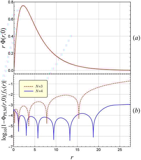
Figure 1.
Negative ion of hydrogen (): (a) the WF, at the electron-nucleus coalescence (the collinear configuration with ) times r; (b) the logarithmic estimates and of the difference (see Equation (17)) between the model WF, and the PLM WF (solid curve, blue online), and between the model WF, and the PLM WF (dashed curve, red online), respectively.
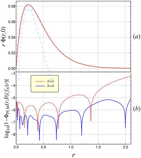
Figure 2.
Ground state of the positive ion of boron (): (a) the WF, at the electron–nucleus coalescence (the collinear configuration with ) times r; (b) the logarithmic estimates and of the difference between the model WF, and the PLM WF (solid curve, blue online), and between the model WF, and the PLM WF (dashed curve, red online), respectively.
It was mentioned earlier that the behavior of the two-electron atomic WF near the nucleus is described by the Fock expansion (6), which reduces to expansion (7) for the collinear arrangement of the particles. The most compact model WFs represented by the sum of three or four exponentials were obtained for the case of the electron-nucleus coalescence corresponding to the collinear parameter . Table 1 and Table 2 together with Figure 1 and Figure 2 demonstrate the high accuracy of those model WFs. It should be emphasized that the accuracy of for is close to the accuracy of the variational PLM WF, for all . Furthermore, the relevant calculations show that the model WF mentioned above is, in fact, more accurate than in the vicinity of nucleus (). We can argue this because the leading terms of the series expansion of (for ) are more close to the corresponding terms of the Fock expansion than the ones for . Actually, Equations (10) and (11) provide by definition the condition and , corresponding exactly to the Fock expansion. Moreover, it is seen from Equation (9)) that for the logarithmic term of the Fock expansion is annihilated because , and hence , where we denoted . One should notice that is, in fact, the single case of the collinear arrangement when the explicit expression for the angular Fock coefficient can be derived in the form [1,22]
where E is the non-relativistic energy of the two-electron atom/ion under consideration. It is seen from Table 5 that (besides ) the values of is much closer to the theoretical values (18) than for all Z. These results confirm the above conclusion about the accuracy of the model WF near the nucleus.
Table 5.
The first and second derivatives of the collinear WF with at the nucleus. The PLM WF, at the electron–nucleus coalescence is introduced.
Author Contributions
All authors contributed equally. All authors have read and agreed to the published version of the manuscript.
Funding
This research received no external funding.
Acknowledgments
This work was supported by the PAZY Foundation, Israel.
Conflicts of Interest
The authors declare no conflict of interest.
References
- Liverts, E.Z.; Krivec, R.; Barnea, N. Collinear configuration of the helium atom and two-electron ions. Ann. Phys. 2020, 422, 168306. [Google Scholar] [CrossRef]
- Amusia, M.Y.; Drukarev, E.G.; Liverts, E.Z.; Mikhailov, A.I. Effects of small recoil momenta in one-photon two-electron ionization. Phys. Rev. A 2013, 87, 043423. [Google Scholar] [CrossRef]
- Amusia, M.Y.; Drukarev, E.G.; Liverts, E.Z. Small recoil momenta double ionization of He and two-electron ions by high energy photons. Eur. Phys. J. D 2020, 74, 173. [Google Scholar] [CrossRef]
- Haftel, M.I.; Mandelzweig, V.B. Fast Convergent Hyperspherical Harmonic Expansion for Three-Body Systems. Ann. Phys. 1989, 189, 29–52. [Google Scholar] [CrossRef]
- Haftel, M.I.; Krivec, R.; Mandelzweig, V.B. Power Series Solution of Coupled Differential Equations in One Variable. J. Comp. Phys. 1996, 123, 149–161. [Google Scholar] [CrossRef][Green Version]
- Pekeris, C.L. Ground State of Two-Electron Atoms. Phys. Rev. 1958, 112, 1649–1658. [Google Scholar] [CrossRef]
- Liverts, E.Z.; Barnea, N. S-states of helium-like ions. Comp. Phys. Comm. 2011, 182, 1790–1795. [Google Scholar] [CrossRef]
- Liverts, E.Z.; Barnea, N. Three-body systems with Coulomb interaction. Bound and quasi-bound S-states. Comp. Phys. Comm. 2013, 184, 2596–2603. [Google Scholar] [CrossRef]
- Hylleraas, E.A. Neue Berechnung der Energie des Heliums im Grundzustande, sowie des tiefsten Terms von Ortho-Helium. Z. Phys. 1929, 54, 347–366. [Google Scholar] [CrossRef]
- Chandrasekhar, S.; Herzberg, G. Energies of the Ground States of He, Li+, and 06+. Phys. Rev. 1955, 98, 1050–1054. [Google Scholar] [CrossRef]
- Kinoshita, T. Ground State of the Helium Atom. Phys. Rev. 1957, 105, 1490–1502. [Google Scholar] [CrossRef]
- Freund, D.E.; Huxtable, B.D.; Morgan, J.D., III. Variational calculations on the helium isoelectronic sequence. Phys. Rev. A 1984, 29, 980–982. [Google Scholar] [CrossRef]
- Frankowski, K.; Pekeris, C.L. Logarithmic Terms in the Wave Functions of the Ground State of Two-Electron Atom. Phys. Rev. 1966, 146, 46–49. [Google Scholar] [CrossRef]
- Korobov, V.I. Coulomb three-body bound-state problem: Variational calculations of nonrelativistic energies. Phys. Rev. A 2000, 61, 064503. [Google Scholar] [CrossRef]
- Frolov, A.M. Multibox strategy for constructing highly accurate bound-state wave functions for three-body systems. Phys. Rev. E 2001, 64, 036704. [Google Scholar] [CrossRef] [PubMed]
- Suzuki, Y.; Varga, K. Stochastic Variational Approach to Quantum-Mechanical Few-Body Problems; Springer: Berlin, Germany; New York, NY, USA; London, UK; Milan, Italy; Paris, France; Tokyo, Japan, 1998. [Google Scholar]
- Drake, G.W.F. High Precision Calculations for Helium, Section 11. In Handbook of Atomic, Molecular, and Optical Physics; Drake, G.W.F., Ed.; AIP Press: New York, NY, USA, 1996. [Google Scholar]
- Nordsieck, A. Reduction of an Integral in the Theory of Bremsstrahlung. Phys. Rev. 1954, 93, 785–787. [Google Scholar] [CrossRef]
- Fock, V.A. On the Schrodinger Equation of the Helium Atom. Izv. Akad. Nauk SSSR Ser. Fiz. 1954, 18, 161–174. [Google Scholar]
- Fadeev, L.D.; Khalfin, L.A.; Komarov, I.V. (Eds.) VA Fock-Selected Works: Quantum Mechanics and Quantum Field Theory; CRC Press: London, UK; Washington, DC, USA, 2004; p. 525. [Google Scholar]
- Abbott, P.C.; Maslen, E.N. Coordinate systems and analytic expansions for three-body atomic wavefunctions: I. Partial summation for the Fock expansion in hyperspherical coordinates. J. Phys. A Math. Gen. 1987, 20, 2043–2075. [Google Scholar] [CrossRef]
- Liverts, E.Z.; Barnea, N. Angular Fock coefficients. Refinement and further development. Phys. Rev. A 2015, 92, 042512. [Google Scholar] [CrossRef]
- Frolov, A.M. On the Q-dependence of the lowest-order QED corrections and other properties of the ground 11S-states in the two-electron ions. Phys. Rev. E 2001, 64, 036704-6. [Google Scholar] [CrossRef]
- Watkins, J.C. An Introduction to the Science of Statistics: From Theory to Implementation, 1st ed.; Topic 13: Method of Moments; 2016; Available online: https://www.math.arizona.edu/~jwatkins/statbook.pdf (accessed on 4 November 2021).
- Liverts, E.Z.; Amusia, M.Y.; Krivec, R.; Mandelzweig, V.B. Boundary solutions of the two-electron Schrodinger equation at two-particle coalescences of the atomic systems. Phys. Rev. A 2006, 73, 012514-9. [Google Scholar] [CrossRef]


Publisher’s Note: MDPI stays neutral with regard to jurisdictional claims in published maps and institutional affiliations. |
© 2021 by the authors. Licensee MDPI, Basel, Switzerland. This article is an open access article distributed under the terms and conditions of the Creative Commons Attribution (CC BY) license (https://creativecommons.org/licenses/by/4.0/).