Abstract
General Relativity is an extremely successful theory, at least for weak gravitational fields; however, it breaks down at very high energies, such as in correspondence to the initial singularity. Quantum Gravity is expected to provide more physical insights in relation to this open question. Indeed, one alternative scenario to the Big Bang, that manages to completely avoid the singularity, is offered by Loop Quantum Cosmology (LQC), which predicts that the Universe undergoes a collapse to an expansion through a bounce. In this work, we use metric gravity to reproduce the modified Friedmann equations which have been obtained in the context of modified loop quantum cosmologies. To achieve this, we apply an order reduction method to the field equations, and obtain covariant effective actions that lead to a bounce, for specific models of modified LQC, considering a massless scalar field.
1. Introduction
1.1. Motivations: Loop Quantum Cosmology and Its Modifications
At the order of the Planck length , where General Relativity (GR) breaks down, a quantum theory of gravity is expected to provide insight on the behaviour of gravity at quantum scales [1], and, consequently, in addressing fundamental open questions [2], such as the initial singularity problem. Loop Quantum Gravity (LQG) [3,4,5] is one of the main candidates, which predicts that classical differential geometry, at small space-time curvatures, is replaced by a discrete quantum geometry at the Planck scale. Indeed, Loop Quantum Cosmology (LQC), which is described as a symmetry-reduced model of LQG [6], provides a more complete understanding of the initial singularity, and through an effective Hamiltonian description yields the following modified Friedmann equation [7,8,9,10,11,12,13]:
where is the Hubble function, given in terms of the scale factor , and the critical energy density is defined as , where is the Barbero–Immirzi parameter [14]. Throughout this work, we use the geometrized system of natural units in which and, accordingly, . The resulting equation of motion is just the usual Friedmann equation, for a spatially flat universe with a cosmological constant equal to zero, with a modified source, which has no extra degrees of freedom compared to GR. The modified Friedmann Equation (1) dictates that the Big Bang singularity is replaced by a quantum bounce that occurs at the critical density , determined by the underlying quantum geometry, which is independent of the matter content of the universe, when and .
Formally, in LQG, the elementary classical phase space variables for the gravitational sector are the Ashtekar–Barbero connection and the conjugate triad . When considering a spatially flat space-time, which is the case in standard LQC, the only relevant constraint is the Hamiltonian constraint, given by [15,16]
whose vanishing yields the equations of motion. is the matter sector constraint and is the gravitational constraint, given by [15,16]
where is the Euclidean term and is the Lorentzian term. The Euclidean part is given by [15,16]
where is the field strength of the connection and det(q) is the determinant of the spatial metric compatible with the triads. The Lorentzian part, on the other hand, is given by [15,16]
where is the extrinsic curvature. Unlike in the framework of full LQG, in the standard LQC scenario, the Euclidean and Lorentzian terms are treated in the same way, due to a classical symmetry reduction, which makes the Lorentzian term a multiple of the Euclidean one. A quantization is then performed on the combination of these two terms, leading to the Hamiltonian constraint in LQC [15]. In this sense, this procedure does not grasp the totality of the full theory of LQG, since the Lorentzian and the Euclidean terms need to be quantized in different ways, leading to a different Hamiltonian constraint. Thus, due to the quantization ambiguities in constructing the Hamiltonian constraint operator in isotropic loop quantum cosmology, this has the important implication that different treatments may arrive at different Planck scale physics. One of the first attempts to understand this problem and to construct a Hamiltonian constraint that is actually similar to the construction in LQG, and inherits more features from the full theory, was undertaken in Ref. [17], in which Thiemann’s regularization was used. Indeed, the Lorentz term of the gravitational Hamiltonian constraint in the spatially flat Friedmann–Lemaître–Robertson–Walker (FLRW) model was quantized by two approaches different from that of the Euclidean term. One of the approaches is very similar to the treatment of the Lorentz part of the Hamiltonian in loop quantum gravity and, therefore, inherits more features from the full theory. Two symmetric Hamiltonian constraint operators were constructed, respectively, in the improved scheme, and it was shown that both have the correct classical limit through the semi-classical analysis. Nevertheless, there is still no systematic derivation of LQC as a cosmological sector of LQG and, as a consequence, different paths to obtain LQG-like Hamiltonians from LQC followed [18,19,20,21]. Due to these quantization ambiguities in constructing the effective Hamiltonian from LQG, it is pertinent to understand how different quantization methods affect the physical predictions. More specifically, there are still great possibilities for the expanding universe to recollapse due to quantum gravity effects.
Throughout this work, we will focus on two specific modified loop quantum cosmology (mLQC) models [15,17], which differ from standard LQC in the way the Lorentzian term in the Hamiltonian constraint is treated [22]. One of the main goals of this study was to verify whether the Big Bang was still replaced by a quantum bounce. Moreover, numerical solutions were shown to be reliable approximations in order to extract phenomenological implications, particularly in the bounce regime.
1.2. Modified Loop Quantum Cosmology—I: mLQC-I
As emphasized in Ref. [15], in LQC it is not necessary to eliminate the Lorentzian term explicitly in order to express the Hamiltonian constraint. In fact, if the Lorentzian term is maintained, different effective Hamiltonians are obtained. In this formal sense, the model derived in Ref. [15], which here we denote by mLQC-I, by treating the Lorentzian term in the Hamiltonian constraint separately and using Thiemann’s regularization [17] yielded a more fundamental difference between LQC and mLQC-I, in that in the latter the evolution of the universe is described by two different branches, and , and, therefore, it is asymmetric with respect to the bounce.
Considering the branch, the modified Friedmann equation takes the form [15,22]
where is the critical density at which the quantum bounce occurs, that is suppressed by a factor of with respect to the standard model of LQC. For , the standard Friedmann equation is recovered.
Concerning the branch, the modified Friedmann equation takes the form [15,22]
where , , and . For this branch, the limit of Equation (7) when , is given by , where . It can be shown that the classical energy conservation law still holds in this modified model of LQC, concerning both branches.
Taking the current cosmological constraints into account, the evolution of the universe must start from the branch, in the pre-bounce phase, and afterwards the evolution will be switched to the one described by the branch. In LQC, we only have one branch due to the fact that the Lorentzian term is not explicit in the Hamiltonian. The two branches coincide at the bounce, [15]. Contrary to the previous branch, in the branch, the quantum geometric effects are still present in the above limit. Comparing with the standard Friedmann equation, we see that these effects are present in the form of a modified Newtonian constant, , and an emergent positive cosmological constant, . These pose phenomenological problems, if this branch lies in the post-bounce universe in which we live [15].
1.3. Modified Loop Quantum Cosmology—Ii: mLQC-II
The second modification of LQC that we consider in this work, outlined in Ref. [17], was derived by using Thiemann’s regularization, similar to the previous model, while using the proportionality of Ashtekar’s connection and extrinsic curvature [16]. The corresponding modified Friedmann equation takes the form [17]
where we find that the quantum bounce occurs at the critical density . Unlike the mLQC-I model, the bounce in this model is perfectly symmetric, as in LQC. However, the modified dynamics in the Planck regime are less trivial, similarly to the mLQC-I model. Another similarity between LQC and mLQC-II is their classical limit. The limit of Equation (8), for , is given by [16]. Once again, using the modified equations that this model provides, the energy–momentum conservation law still holds without any change in the properties of the equation of state (EoS).
1.4. Order Reduction
Now, the only covariant action that leads to second-order equations, under metric variation, is the Einstein–Hilbert (EH) action, and any change in this action leads to higher-order equations. Considering an action other than the one from GR appears to be unjustified given that it implies a departure of a framework that has proven to be successful in describing several physical phenomena. However, considering such theories might be useful, especially if they are close to the theory which we believe to be presently more correct. In fact, given that the modified Friedmann Equations (6)–(8) are obtained from modified sources, a reasonable question to ask is whether it is possible to derive them from an effective action, other than the EH action. An interesting analysis was considered in the Palatini approach of gravity in Ref. [23]. In this context, the functional Palatini is a function of the trace of the energy–momentum tensor T, so that the modified Friedmann equation in Palatini gravity does not involve any higher derivatives of the geometrical quantities and is just a function of the matter sources [24]. Indeed, this result provided new insights on the continuum properties of the discrete structure of quantum geometry. In this work, in order to deduce effective actions, we use metric gravity [25,26,27,28,29,30,31], where the full field equations in this framework are of fourth-order. One advantage of using gravity is that this theory seems to be the only one which can avoid the Ostrogradski instability [29,32]. We can either consider this theory as an exact theory, meaning that their field equations are considered as genuinely higher-order, or we can treat it as an effective field theory by only considering the solutions which are perturbatively close to GR as the physical ones and the rest as spurious [33,34,35]. A method that provides the latter approach is that of covariant order reduction, which allows one to find solutions that are perturbatively close to GR. A further advantage of this procedure consists in the fact that it may also serve as a model selection approach. The idea of considering only the solutions which are perturbatively close to GR is not new in cosmology. For example, an inflation model with a polynomial expression for was phenomenologically investigated in [36]. Another example is presented in [37], where the inflationary model was considered by treating the term as a small perturbation.
Indeed, it was shown that, at least for isotropic models in LQC, using a covariant order reduction then a covariant effective action can be found if one considers higher-order theories of gravity but faithfully follows effective field theory techniques [32]. In this context, these techniques were applied within bouncing cosmologies, which can be envisaged as candidates for solving the Big Bang initial singularity problem. In Ref. [38], bouncing solutions in a modified Gauss–Bonnet gravity theory were explored, of the type , where R is the Ricci scalar, G is the Gauss–Bonnet term, and f is some function of it [38]. In finding such a bouncing solution, the order reduction technique was used to reduce the order of the differential equations of the theory to second order equations. As GR is a theory whose equations are of second order, this order reduction technique enables one to find solutions which are perturbatively close to GR. Furthermore, the covariant action of the order reduced theory was also obtained. The analysis explored in Ref. [38] was extended in the context of gravity by using the same order reduction technique [39]. Indeed, several covariant gravitational actions leading to a bounce are directly selected by demanding that the Friedmann equation derived within such gravity theories coincides with the one emerging from LQC. The same approach has also been implemented in the context of symmetric teleparallel gravity theories, where Q is the non-metricity scalar [40]. Further cases were explored in Refs. [41,42].
1.5. Outline of the Paper
In this work, we are interested in extending the analysis outlined in Ref. [32], by applying the method of covariant order reduction to the modified Friedmann Equations (6)–(8), within the modified loop quantum cosmologies considered above. To this effect, we write out the Lagrangian density of gravity as the sum of the gravitational Lagrangian of GR and a deviation term, and present the final form of the reduced modified Friedmann equations. In Section 2, we present the covariant order reduction technique in some detail and outline a strategy to deduce the effective actions. In Section 3, we obtain the effective actions for the modified loop quantum cosmological models considered above. Finally, in Section 4, we conclude and discuss our results.
2. Covariant Order Reduction Technique
2.1. Reduced Equations in Gravity
In this work, we consider metric gravity, whose corresponding action is given by
where g is the determinant of the metric tensor , is the matter action defined as , being the matter Lagrangian density, in which matter is minimally coupled to the metric , and collectively denotes the matter fields. Without loss of generality, we parametrize the Lagrangian density as the sum of the gravitational Lagrangian of GR and a deviation term, as follows
where is the cosmological constant, is a dimensionless parameter, and represents the deviation from GR. Substituting Equation (10) in Equation (9), and varying the action with respect to the metric yields the following gravitational field equations
The energy–momentum tensor is defined as
We now apply the order reduction technique to Equation (11). In the present case, this amounts to replacing the Ricci scalar and the Ricci tensor, in the terms of order , by the expression we obtain from them, from the version of the same equations. Thus, setting in Equation (11), yields the following
as the reduced expression of the Ricci tensor, where is the order reduced Ricci scalar. Taking into account the trace of Equation (13), the latter provides , and after substituting it into Equation (13), we arrive at
Replacing R and , in the -order terms in Equation (11), with the above expressions, we finally obtain
These are reduced field equations in the sense that we are not using the complete field equations to determine expressions for R and . We should notice that this approximation is only valid when
After a solution is determined, it has to be verified a posteriori for which interval of values of R this is valid.
Throughout this work, we consider an isotropic and homogeneous universe described by the FLRW metric with a signature, which, in spherical coordinates, is given by
where is the scale factor and k is the curvature of the universe, which can be set equal to , 0, or , depending if one is considering a hyperspherical, spatially flat, or hyperbolic universe, respectively. We assume a perfect fluid description for the content of the universe, given by the energy–momentum tensor, , where is the four-velocity field of an observer comoving with the fluid, defined in such a way that , and and are the fluid’s energy density and isotropic pressure, respectively.
Now, taking into account the FLRW metric (17), then Equation (15) provides the following modified Friedmann equation
by taking into account a barotropic EoS , with . Note that we recover the standard Friedmann equation for .
In the context of the order reduction method, we substitute the term within the term on the right hand side of Equation (18) by the standard Friedmann equation, which yields [32]
as our final form of the reduced modified Friedmann equation in gravity. It is clear now, that the reduced differential equation is effectively a second-order one. With this result, we aim to find a function , such that Equation (19) is the same as some Friedmann equation with a modified source.
2.2. Strategy to Obtain Effective Actions
Here, we specify the conditions in which we will be using Equation (19). In this context, we consider a spatially flat universe () with a zero cosmological constant (), so that . Taking these aspects into account, then Equation (19) becomes
In the following sections, we will compare Equation (20) to the modified Friedmann Equations (6)–(8) considered in the modified loop quantum cosmologies, outlined in the Introduction. However, we reinforce the idea that there are two kinds of modified Friedmann equations at play. One of them is Equation (20), which was derived in the context of metric gravity, and the other one was derived in the context of LQC. Thus, our main goal is to determine , such that Equation (20) is the same as Equations (6)–(8). In doing so, we will determine an effective action that leads to the quantum bounce which characterizes those models. Thus, the modified Friedmann equation, in the context of LQC and its modifications, can be written, in a general way, as
where is some algebraic function, which will depend on the model. Comparing with Equation (20), the requirement is that satisfies
for a given . The same equation, written in terms of , using , is given by
For each model, mLQC-I and mLQC-II, we will be considering the scenario of a massless scalar field (). In this context, an effective action for LQC was already determined in Ref. [32].
3. Effective Actions for Modified Loop Quantum Cosmology Models
In order to be in agreement with the approach leading to Equation (1), we consider a massless scalar field, i.e., we set the EoS parameter to be . Therefore, Equation (20) simplifies to
and, as a consequence, Equation (22) reduces to
with
Note that is negative, as the energy density is positive. Finally, we write out Equation (25) in terms of as
Independently of the model of LQC that we are considering, at a given moment, the solution to the non-homogeneous Equation (27) consists of the sum of the solution to the corresponding homogeneous equation and its particular solution,
As such, before specifying any of the models, by substituting in Equation (27) for each case, let us consider the homogeneous equation first, which is common to all cases and is given by
This equation is a homogeneous second order Cauchy–Euler equation, having the form
Assuming a trial solution, gives
We now see that was a rather natural choice since we obtained a common factor that we can drop obtaining the characteristic equation for m, given by . Through the roots of this equation, we obtain a solution for Equation (30) whose form depends on the number of roots, and if they are real or complex. In the present case, the characteristic equation for the homogeneous Equation (29) is and, solving for m, one obtains two real roots, , meaning that the solution to Equation (29) is given by
This solution does not contain analytic functions of R, meaning it is not locally given by a convergent power series. For this reason, and also for the fact that does not contribute to the full Equation (27), we can set , without loss of generality [32]. As such, the solutions to Equation (27) are simply given by the particular solution in question
depending on .
3.1. Effective Action for LQC
Here, for self-completeness and self-consistency, we briefly present the particular scenario studied in Ref. [32], where an effective action for LQC was found, requiring matter to be a scalar field, in order to be in agreement with the approach leading to Equation (1) [13]. From Equation (21), for LQC we have that or, as a function of , using , we have . Therefore, in this case, Equation (27) is given by
Since we already covered the solution to Equation (29), we now focus on its particular solution. Looking at Equation (34), the particular solution should be of the form , where A is a constant. Plugging this in Equation (34) and solving for A, one obtains . We therefore have [32]:
where we have dropped the subscript T since, to order, and are the same. Thus, the function for the effective action, that leads to Equation (1), is [32]
where the dots are an indication of an infinite series. Notice that the case of a quadratic model , in the context of LQC, was also considered in Ref. [43]. An effective brane-world and the LQC background expansion histories were also reproduced from a modified gravity perspective in terms of a quadratic term in the Ricci scalar, in a theory non-minimally coupled with the matter Lagrangian [44]. We can neglect the rest of the terms, as they are subdominant with respect to the quadratic term. According to the order reduction method, this solution is only valid for a certain range of curvatures, given by Equation (16), or, equivalently, for a certain range of energy density values. In this case, the solution is valid for
Thus, a metric action was found in Ref. [32] which, when treated as an effective action, leads to the modified Friedmann equation, provided by LQC. Here, we follow an analogous procedure for the modified models of LQC.
3.2. Effective Actions for mLQC-I
As described in the Introduction, mLQC-I is divided in two branches. As such, we consider each of them separately and find an effective action for both.
3.2.1. Effective Action for the Branch
Considering Equation (6) for the branch, we find that Equation (21), in this case, is given by
or, using Equation (26),
Therefore, in this case, Equation (27) provides
Using Wolfram Mathematica, we obtain the following solution
where, again, we have dropped the subscript T since, to order, and are the same.
As expected, the first two terms in Equation (41) correspond to Equation (32), and the remaining terms correspond to the particular solution to Equation (40). This solution contains hypergeometric functions1, denoted by , and its domain is . Along with the fact that it only makes physical sense that , we have that our physical solution is defined in the range
Thus, a metric action was found which, when treated as an effective action, leads to the modified Friedmann Equation (7), provided by the branch of mLQC-I. Setting , without loss of generality, the effective action is given by
Using Wolfram Mathematica, a Taylor expansion of Equation (45), about and up to third order, was computed and is given by
where the critical density for this model is given by
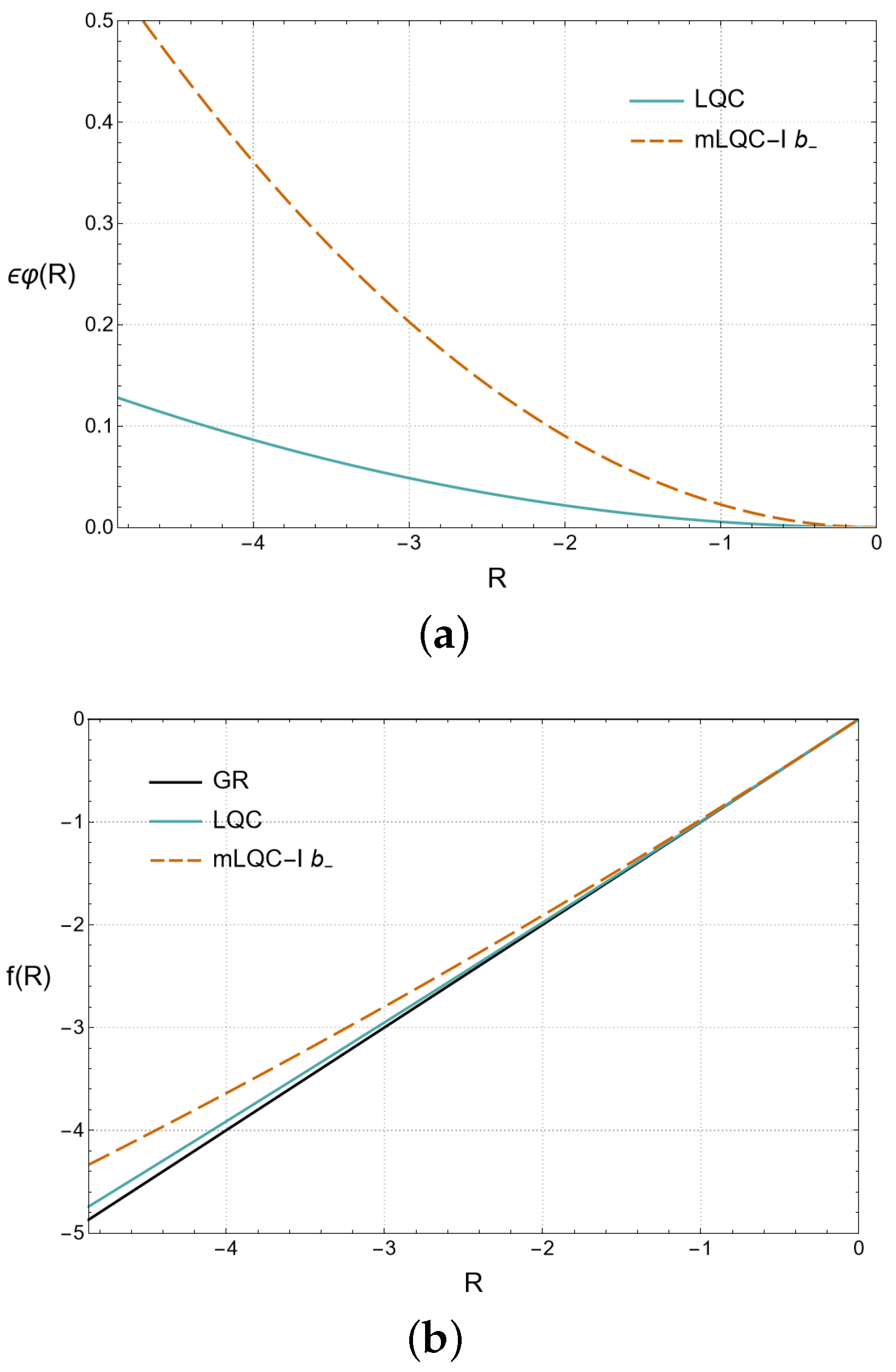
In order to better convey the magnitude of the deviation from GR in this case, we provide two different plots in Figure 1. In Figure 1a, we present the deviation of the effective Lagrangian density from the one we find in GR, as a function of R. In this plot, we are able to compare the deviation in the case of LQC, given by Equation (35), with that of mLQC-I, in the case of branch. Notice that we are plotting Equation (41), with , not the corresponding series expansion. In Figure 1b, we compare the effective functions of LQC and the branch of mLQC-I, given by Equations (36) and (45), respectively, with that of GR, with .
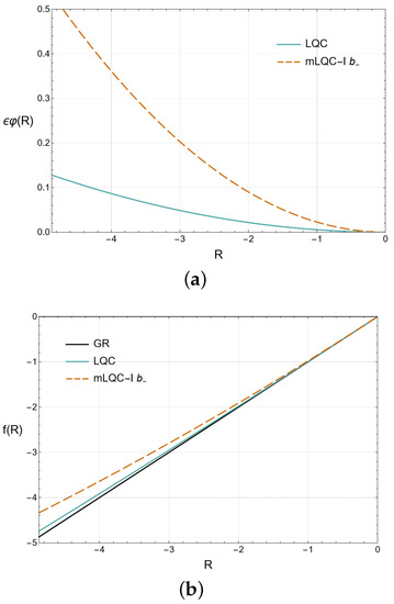
Figure 1.
The plot (a) (Deviation, from GR, of the effective Lagrangian: a comparison between the branch of mLQC-I and LQC) presents the comparison between Equation (41), for the branch of mLQC-I (dashed dark orange line), and Equation (35), for LQC (solid blue line), with , for . Although the deviation is higher for the case of the branch of this modified model, both of them are dominated by the quadratic term. The plot (b) (Effective function: a comparison between the branch of mLQC-I, LQC, and GR) illustrates the differences between the Lagrangian density of GR (solid black line), with , and the effective Lagrangian densities given by Equation (36), in the case of LQC (solid blue line) and Equation (45), for the branch of mLQC-I (dashed dark orange line), for the interval .
3.2.2. Effective Action for the Branch
Considering the branch, with the modified Friedmann Equation (6), we find that Equation (21) is given by
or, using Equation (26),
Therefore, in this case Equation (27) becomes
where . As before, the solution to Equation (50) was obtained using Wolfram Mathematica, and is given by
where we have dropped the subscript T since, to order, and are the same. Once again, the first two terms correspond to Equation (32), and the remaining ones correspond to the particular solution of Equation (50). As in the previous branch, the solution contains hypergeometric functions and its domain is given by . As such, since it only makes physical sense that , Equation (51) is defined, as a physical solution, for the range
Taking the same argument as in the previous calculations, we can set and, as a consequence, the effective action is given by
A Taylor expansion of Equation (53) up to third order, about , was computed using Wolfram Mathematica, resulting in
We observe that, for this particular branch, . We recall that was interpreted as the energy density of an emergent positive cosmological constant in Ref. [15].
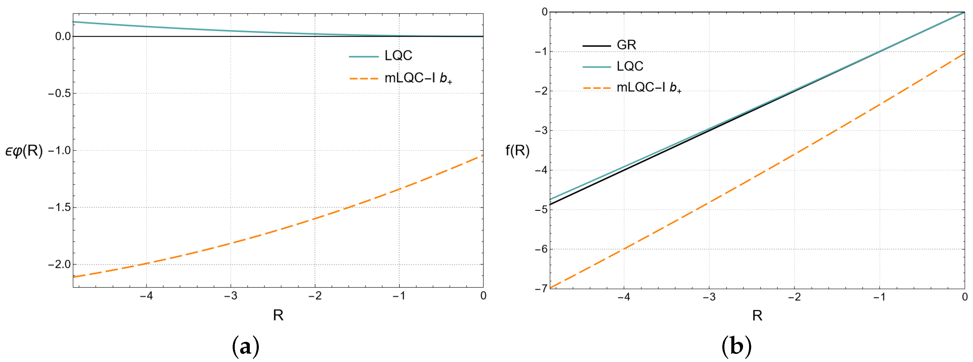
Thus, a metric action was also found for the branch of mLQC-I which, when treated as an effective action, leads to the modified Friedmann Equation (7). Finally, using the same definitions we used before, to provide plots for the branch, we also provide the same kind of plots for this branch, in Figure 2. In Figure 2a, we can observe that, for mLQC-II, is an increasing function, contrary to all the other models we are considering.
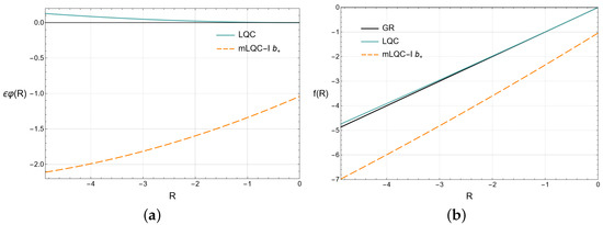
Figure 2.
The plot (a) (Deviation, from GR, of the effective Lagrangian: a comparison between the branch of mLQC-I and LQC) presents the comparison between Equation (51), for the branch of mLQC-I (dashed light orange line), and Equation (35), for LQC (solid blue line), with , for . Contrary to the previous case, for this branch the correction is dominated by the linear term. As a result, since , the deviation is predominantly negative. The plot (b) (Effective function: a comparison between the branch of mLQC-I, LQC, and GR) illustrates the differences between the Lagrangian density of GR (solid black line), with , and the effective Lagrangian densities given by Equation (36), in the case of LQC (solid blue line), and Equation (53), for the branch of mLQC-I (dashed light orange line), for the interval .
3.3. Effective Action for mLQC-II
We now consider the mLQC-II model, in which the modified Friedmann equation is given by Equation (8). In this case, Equation (21) is given by
or, using Equation (26),
Therefore, in this case Equation (27) is given by
The solution to Equation (57) was obtained using Wolfram Mathematica, and leads to
where we have dropped the subscript T since, to order , , and are the same. As usual, the first two terms correspond to Equation (32) and the remaining terms correspond to the particular solution of Equation (57). For this model, the solution also contains hypergeometric functions but with a different argument and its domain is given by . As such, in this case the solution only has physical meaning for the interval
Thus, a metric action was found which, when treated as an effective action, leads to the modified Friedmann Equation (8), provided by mLQC-II. Setting this effective action is given by
Using Wolfram Mathematica, a Taylor expansion of Equation (60), about and up to third order, was computed and is given by
where the critical density for this model is
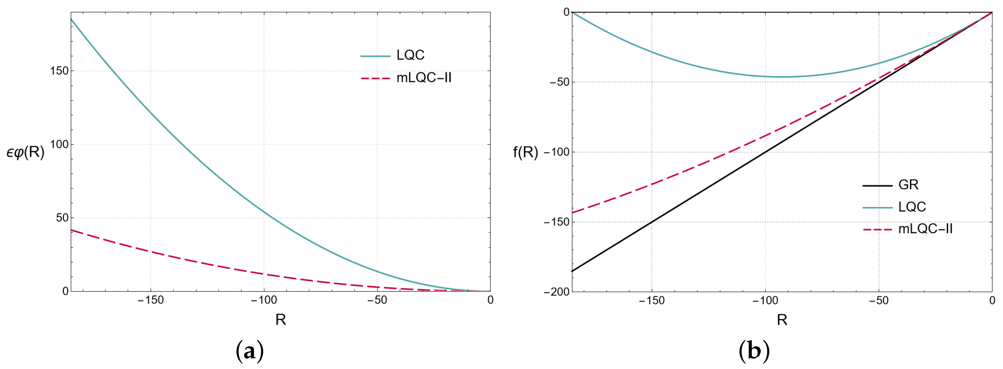
This solution for the mLQC-II model is depicted in Figure 3. In Figure 3a, we present the deviation of the effective Lagrangian density from the general relativistic counterpart, and compare them to the the deviation in the case of LQC, given by Equation (35), with that of mLQC-II, given by Equation (41) with . In Figure 3b, we compare the effective functions of LQC and mLQC-II, given by Equation (36) and Equation (60), respectively, with that of GR, with .
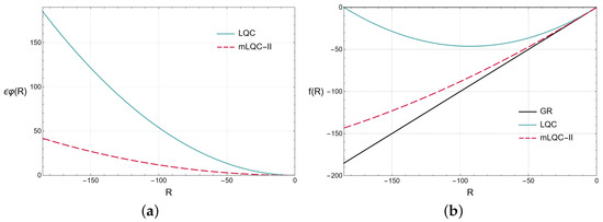
Figure 3.
The plot (a) (Deviation, from GR, of the effective Lagrangian: a comparison between mLQC-II and LQC) presents the comparison between Equation (58), for the case of mLQC-II (dashed pink line), and Equation (35), for LQC (solid blue line), with , for . Both of the corrections are dominated by the quadratic term. The plot (b) (Effective function: a comparison between mLQC-II, LQC, and GR) illustrates the differences between the Lagrangian density of GR (solid black line), with , and the effective Lagrangian densities, in the case of LQC (solid blue line), and Equation (60), for mLQC-II (dashed pink line), for the interval .
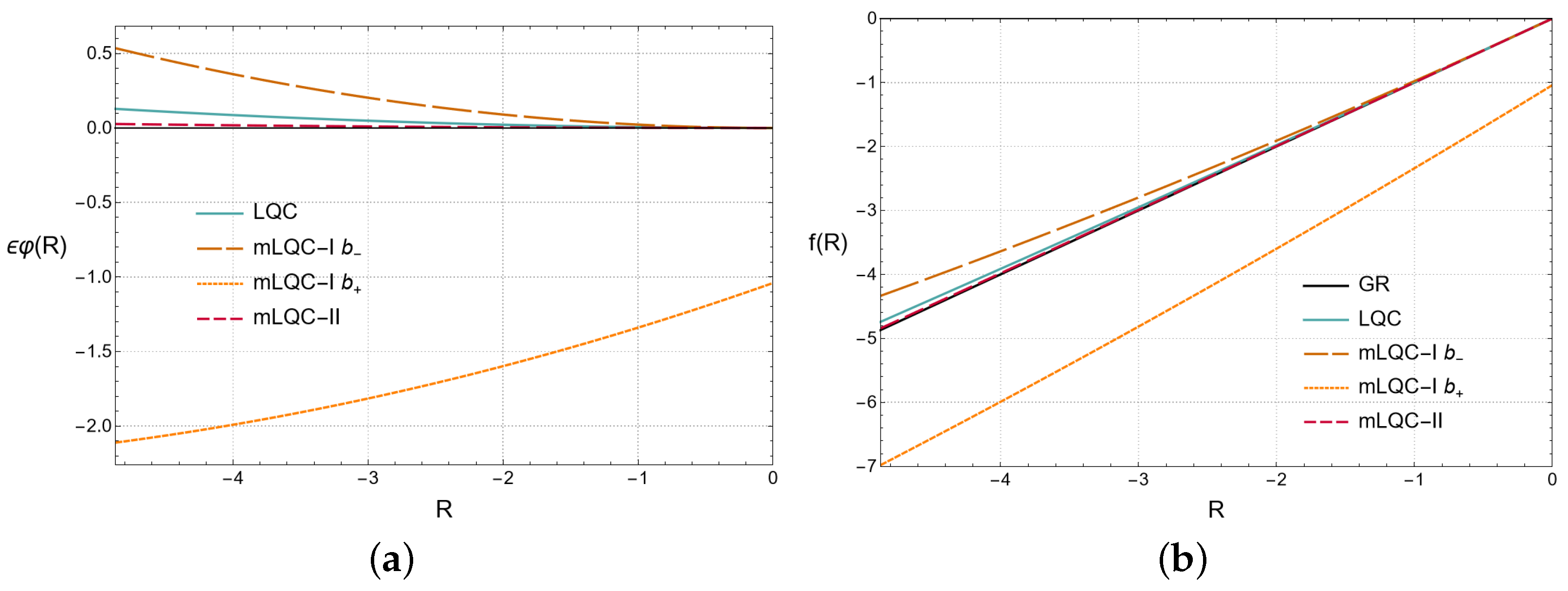
Finally, we also present in Figure 4 two plots with all the solutions. In Figure 4a, we compare all the deviations with respect to the Lagrangian density of GR. In Figure 4b, all the effective metric functions are displayed. With the exception of the branch of mLQC-I, all deviations from GR are dominated by the quadratic term and the remaining terms become more subdominant, with increasing order, as is the case in LQC. In the case of the branch, the dominant term is linear, due to the presence of the constant on the right-hand side of Equation (50), which is not the case in any of the other equations we have solved.
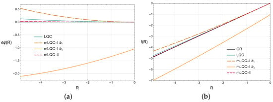
Figure 4.
The plot (a) (Deviation, from GR, of the effective Lagrangian: a comparison between all models) contains Equation (35), for LQC (solid blue line), Equation (41), for the branch of mLQC-I (dashed dark orange line), Equation (51), for the branch of mLQC-I (dashed light orange line) and Equation (58), for mLQC-II (dashed pink line), with , for . The plot (b) (Effective function: a comparison between all models) presents the effective functions for all models, including GR (solid black line), with . These are Equation (36), for LQC (solid blue line), Equation (45), for the branch of mLQC-I (dashed dark orange line), Equation (53), for branch of mLQC-I (dashed light orange line) and Equation (60), for mLQC-II (dashed pink line), for .
4. Conclusions
In this work, we have addressed the initial singularity problem that is present in the ΛCDM model, in which the Universe emerges from a single point with infinite density, and considered a possible resolution to this question, as proposed by LQC, in which the Big Bang is replaced by a quantum bounce. Through an effective Hamiltonian description, this bounce is manifested by an effective Friedmann equation that is similar to the one found in GR, but with a modified source, given by Equation (1). It is clear from this equation that the energy density reaches a finite maximum value, a critical density, contrary to the Big Bang scenario. In this regard, LQC proposes a scenario in which the Universe undergoes a collapse to an expansion through a bounce.
Since this result comes from a different field in physics, it is relevant to ask if it is possible to replicate it in the framework of GR and its modifications. In this context, in order to obtain the modified Friedmann Equation (1), we considered the class of metric gravity, where the Ricci scalar in the EH action, is substituted by a general function of R. Using this particular modification of GR, an effective action that leads to Equation (1) was determined in Ref. [32], assuming a massless scalar field. Motivated by this approach, we considered two modifications of standard LQC, which also yield a quantum bounce that occurs for a critical density, specific to each model, which we denoted by mLQC-I and mLQC-II, as outlined in the Introduction. These modifications came to be formulated as a result of a departure of LQC from LQG. More specifically, in LQC, which is a symmetry-reduced model of LQG, the different components of the Hamiltonian are treated as multiples of each other. This is not the case in the full theory of LQG. As such, mLQC-I and mLQC-II are two attempts to incorporate more aspects of LQG in LQC, by means of similar treatments of the Hamiltonian, with respect to the treatment given in LQG.
Furthermore, we applied the covariant order reduction method by obtaining a reduced version of the full field equations of gravity, in the sense that they are second-order equations and give solutions perturbatively close to GR, and deduced the modified Friedmann equations. This equation depends on the function, which we chose to parametrize as . Motivated by the example given in Ref. [32], in which a function was found, we applied this procedure to the mLQC-I and mLQC-II models. The first model, mLQC-I, is divided in two branches, denoted by and , providing the modified Friedmann equations given by Equations (6) and (7), respectively. The second model, mLQC-II, gives the modified Friedmann Equation (8). Using the software Wolfram Mathematica, we then found a function , such that Equations (6)–(8) are the same as Equation (20), for . As such, specific effective covariant actions were found, in the context of metric gravity, which provide Equations (6)–(8), for , according to Equation (16). These effective actions satisfy , allowing for a positive effective gravitational coupling, and , avoiding the Dolgov–Kawasaki instability [25].
The approach followed in this article breaks down in regions of very high energy densities, which are the most interesting regions for physics and phenomenology. Indeed, the approximation that we use is valid for , breaking down at , since . Thus, the argument that the effective Lagrangians deduced in this work yield Equations (6)–(8) is not quite a rigorous statement. However, our claim is that at stages close enough to the bounce, such as just before and after it, the Lagrangians found in this work may effectively and correctly describe the collapsing universe. Moreover, it should be noted that the modified Friedmann equations derived in this paper are not guaranteed to respect general covariance, a problem that remains open in LQC models that involve quantum bounces [45].
We would like to point out that there is a simpler approach compared to the one presented in this paper, namely gravity [46], where is an invariant, such as the torsion, the intrinsic curvature, a combination of the Carminati–McLenaghan, or the invariant coming from mimetic gravity which, at the background level, mimics standard LQC [47]. This approach could, in principle, be applied to the modifications of LQC, providing simpler formulations than those obtained in the present paper. Moreover, in some works dealing with gravity, it has been reported that the corresponding equations do not coincide with the ones of LQC and, in fact, they can lead to the Ostrogradski instability, as opposed to gravity theories [29,32], or gradient instability, as well as to the appearance of ghost fields. A similar conclusion could be obtained for modified LQC at the perturbations level.
A successful theory that combines GR and quantum mechanics is yet to be found. In order to predict and describe the beginning of the Universe, we need physical laws that are valid in that regime. If GR is the correct theory in describing the Universe in that period, then the singularity theorem would show that, in the beginning, the Universe was contained in a single point, with infinite density and infinite curvature. However, what the theorem really shows is that, in the beginning of time, the magnitude of the gravitational interaction was so strong, that quantum gravitational effects were, most likely, relevant. As such, it is expected that a quantum theory of gravity will allow for a proper description of the beginning of the Universe. In this regard, the ΛCDM model is incomplete and, for this reason, it is pertinent to attempt modifications of GR, in order to accommodate scenarios in which the Big Bang singularity is non-existent, such as the covariant effective actions determined in this work. In a forthcoming paper we will extend our analysis to arbitrary values of w for mLQC–II.
Author Contributions
Formal analysis, A.R.R., D.V. and F.S.N.L.; Investigation, A.R.R., D.V. and F.S.N.L.; Writing original draft, A.R.R., D.V. and F.S.N.L. All the authors have substantially contributed to the present work. All authors have read and agreed to the published version of the manuscript.
Funding
This research was funded by the Fundação para a Ciência e a Tecnologia (FCT) from the research grants UIDB/04434/2020, UIDP/04434/2020 and CERN/FIS-PAR/0037/2019 and PTDC/FIS-AST/0054/2021.
Institutional Review Board Statement
Not applicable.
Informed Consent Statement
Not applicable.
Data Availability Statement
Not applicable.
Acknowledgments
D.V. acknowledges support from the Istituto Nazionale di Fisica Nucleare (INFN) (iniziativa specifica TEONGRAV). F.S.N.L. acknowledges support from the Fundação para a Ciência e a Tecnologia (FCT) Scientific Employment Stimulus contract with reference CEECINST/00032/2018, and funding from the research grants UIDB/04434/2020, UIDP/04434/2020 and CERN/FIS-PAR/ 0037/2019. D.V. and F.S.N.L. also acknowledge support from the grant PTDC/FIS-AST/0054/2021.
Conflicts of Interest
The authors declare no conflict of interest.
Note
| 1 | The Gaussian, or ordinary hypergeometric function, is a special function defined by the hypergeometric series
|
References
- Amelino-Camelia, G. Quantum-Spacetime Phenomenology. Living Rev. Relativ. 2013, 16, 1–137. [Google Scholar] [CrossRef]
- Carlip, S. Quantum gravity: A Progress report. Rep. Prog. Phys. 2001, 64, 885. [Google Scholar] [CrossRef]
- Rovelli, C. Loop quantum gravity. Living Rev. Relativ. 2008, 11, 1–69. [Google Scholar] [CrossRef]
- Thiemann, T. Modern Canonical Quantum General Relativity; Cambridge University Press: Cambridge, UK, 2008. [Google Scholar]
- Ashtekar, A.; Lewandowski, J. Background independent quantum gravity: A Status report. Class. Quantum Gravity 2004, 21, R53. [Google Scholar] [CrossRef]
- Bojowald, M. Loop quantum cosmology. Living Rev. Relativ. 2008, 11, 1–131. [Google Scholar] [CrossRef] [PubMed]
- Bojowald, M. Absence of singularity in loop quantum cosmology. Phys. Rev. Lett. 2001, 86, 5227. [Google Scholar] [CrossRef] [PubMed]
- Ashtekar, A.; Pawlowski, T.; Singh, P. Quantum Nature of the Big Bang: An Analytical and Numerical Investigation. Phys. Rev. D 2006, 73, 124038. [Google Scholar] [CrossRef]
- Ashtekar, A.; Pawlowski, T.; Singh, P. Quantum Nature of the Big Bang: Improved dynamics. Phys. Rev. D 2006, 74, 84003. [Google Scholar] [CrossRef]
- Taveras, V. Corrections to the Friedmann Equations from LQG for a Universe with a Free Scalar Field. Phys. Rev. D 2008, 78, 64072. [Google Scholar] [CrossRef]
- Banerjee, K.; Calcagni, G.; Martin-Benito, M. Introduction to loop quantum cosmology. SIGMA 2012, 8, 16. [Google Scholar] [CrossRef]
- De Haro, J.; Amorós, J. Bouncing cosmologies via modified gravity in the ADM formalism: Application to Loop Quantum Cosmology. Phys. Rev. D 2018, 97, 64014. [Google Scholar] [CrossRef]
- Singh, P. Loop cosmological dynamics and dualities with Randall-Sundrum braneworlds. Phys. Rev. D 2006, 73, 63508. [Google Scholar] [CrossRef]
- Meissner, K.A. Black hole entropy in loop quantum gravity. Class. Quantum Gravity 2004, 21, 5245. [Google Scholar] [CrossRef]
- Li, B.F.; Singh, P.; Wang, A. Towards Cosmological Dynamics from Loop Quantum Gravity. Phys. Rev. D 2018, 97, 84029. [Google Scholar] [CrossRef]
- Li, B.F.; Singh, P.; Wang, A. Qualitative dynamics and inflationary attractors in loop cosmology. Phys. Rev. D 2018, 98, 66016. [Google Scholar] [CrossRef]
- Yang, J.; Ding, Y.; Ma, Y. Alternative quantization of the Hamiltonian in loop quantum cosmology II: Including the Lorentz term. Phys. Lett. B 2009, 682, 1–7. [Google Scholar] [CrossRef]
- Dapor, A.; Liegener, K. Cosmological Effective Hamiltonian from full Loop Quantum Gravity Dynamics. Phys. Lett. B 2018, 785, 506–510. [Google Scholar] [CrossRef]
- Dapor, A.; Liegener, K. Cosmological coherent state expectation values in loop quantum gravity I. Isotropic kinematics. Class. Quantum Gravity 2018, 35, 135011. [Google Scholar] [CrossRef]
- Alesci, E.; Barrau, A.; Botta, G.; Martineau, K.; Stagno, G. Phenomenology of Quantum Reduced Loop Gravity in the isotropic cosmological sector. Phys. Rev. D 2018, 98, 106022. [Google Scholar] [CrossRef]
- Bilski, J.; Marcianò, A. Critical Insight into the Cosmological Sector of Loop Quantum Gravity. Phys. Rev. D 2020, 101, 66026. [Google Scholar] [CrossRef]
- Li, B.F.; Singh, P.; Wang, A. Genericness of pre-inflationary dynamics and probability of the desired slow-roll inflation in modified loop quantum cosmologies. Phys. Rev. D 2019, 100, 63513. [Google Scholar] [CrossRef]
- Olmo, G.J.; Singh, P. Effective Action for Loop Quantum Cosmology a la Palatini. J. Cosmol. Astropart. Phys. 2009, 2009, 30. [Google Scholar] [CrossRef]
- Olmo, G.J. Palatini Approach to Modified Gravity: f(R) Theories and Beyond. Int. J. Mod. Phys. D 2011, 20, 413–462. [Google Scholar] [CrossRef]
- Sotiriou, T.P.; Faraoni, V. f(R) Theories Of Gravity. Rev. Mod. Phys. 2010, 82, 451. [Google Scholar] [CrossRef]
- Lobo, F.S.N. The Dark side of gravity: Modified theories of gravity. arXiv 2008, arXiv:0807.1640. [Google Scholar]
- De Felice, A.; Tsujikawa, S. f(R) theories. Living Rev. Relativ. 2010, 13, 1–161. [Google Scholar] [CrossRef] [PubMed]
- Nojiri, S.; Odintsov, S.D. Unified cosmic history in modified gravity: From f(R) theory to Lorentz non-invariant models. Phys. Rep. 2011, 505, 59–144. [Google Scholar] [CrossRef]
- Clifton, T.; Ferreira, P.G.; Padilla, A.; Skordis, C. Modified Gravity and Cosmology. Phys. Rep. 2012, 513, 1–189. [Google Scholar] [CrossRef]
- Capozziello, S.; De Laurentis, M. Extended Theories of Gravity. Phys. Rep. 2011, 509, 167–321. [Google Scholar] [CrossRef]
- Harko, T.; Lobo, F.S.N. Extensions of f(R) Gravity: Curvature-Matter Couplings and Hybrid Metric-Palatini Theory. In Cambridge Monographs on Mathematical Physics; Cambridge University Press: Cambridge, UK, 2018. [Google Scholar]
- Sotiriou, T.P. Covariant Effective Action for Loop Quantum Cosmology from Order Reduction. Phys. Rev. D 2009, 79, 44035. [Google Scholar] [CrossRef]
- Bel, L.; Zia, H.S. Regular reduction of relativistic theories of gravitation with a quadratic Lagrangian. Phys. Rev. D 1985, 32, 3128–3135. [Google Scholar] [CrossRef] [PubMed]
- Simon, J.Z. Higher Derivative Lagrangians, Nonlocality, Problems and Solutions. Phys. Rev. D 1990, 41, 3720. [Google Scholar] [CrossRef]
- Simon, J.Z. No Starobinsky inflation from selfconsistent semiclassical gravity. Phys. Rev. D 1992, 45, 1953–1960. [Google Scholar] [CrossRef]
- Huang, Q.G. A polynomial f(R) inflation model. J. Cosmol. Astropart. Phys. 2014, 2, 35. [Google Scholar] [CrossRef]
- Castellanos, A.R.R.; Sobreira, F.; Shapiro, I.L.; Starobinsky, A.A. On higher derivative corrections to the R + R2 inflationary model. J. Cosmol. Astropart. Phys. 2018, 12, 7. [Google Scholar] [CrossRef]
- Terrucha, I.; Vernieri, D.; Lemos, J.P.S. Covariant action for bouncing cosmologies in modified Gauss–Bonnet gravity. Ann. Phys. 2019, 404, 39–46. [Google Scholar] [CrossRef]
- Barros, B.J.; Teixeira, E.M.; Vernieri, D. Bouncing cosmology in f(R,) gravity by order reduction. Ann. Phys. 2020, 419, 168231. [Google Scholar] [CrossRef]
- Bajardi, F.; Vernieri, D.; Capozziello, S. Bouncing Cosmology in f(Q) Symmetric Teleparallel Gravity. Eur. Phys. J. Plus 2020, 135, 912. [Google Scholar] [CrossRef]
- Miranda, M.; Vernieri, D.; Capozziello, S.; Lobo, F.S.N. Effective actions for loop quantum cosmology in fourth-order gravity. Eur. Phys. J. C 2021, 81, 975. [Google Scholar] [CrossRef]
- Miranda, M.; Vernieri, D.; Capozziello, S.; Lobo, F.S.N. Bouncing Cosmology in Fourth-Order Gravity. Universe 2022, 8, 161. [Google Scholar] [CrossRef]
- Amorós, J.; de Haro, J.; Odintsov, S.D. R + αR2 Loop Quantum Cosmology. Phys. Rev. D 2014, 89, 104010. [Google Scholar] [CrossRef]
- Olmo, G.J.; Rubiera-Garcia, D. “Brane-world and loop cosmology from a gravity–matter coupling perspective. Phys. Lett. B 2015, 740, 73–79. [Google Scholar] [CrossRef]
- Bojowald, M. Noncovariance of the dressed-metric approach in loop quantum cosmology. Phys. Rev. D 2020, 102, 23532. [Google Scholar] [CrossRef]
- Bernal, T.; Capozziello, S.; Hidalgo, J.C.; Mendoza, S. Recovering MOND from extended metric theories of gravity. Eur. Phys. J. C 2011, 71, 1794. [Google Scholar] [CrossRef]
- de Haro, J.; Aresté Saló, L.; Pan, S. Limiting curvature mimetic gravity and its relation to Loop Quantum Cosmology. Gen. Relativ. Gravit. 2019, 51, 49. [Google Scholar] [CrossRef]
Disclaimer/Publisher’s Note: The statements, opinions and data contained in all publications are solely those of the individual author(s) and contributor(s) and not of MDPI and/or the editor(s). MDPI and/or the editor(s) disclaim responsibility for any injury to people or property resulting from any ideas, methods, instructions or products referred to in the content. |
© 2023 by the authors. Licensee MDPI, Basel, Switzerland. This article is an open access article distributed under the terms and conditions of the Creative Commons Attribution (CC BY) license (https://creativecommons.org/licenses/by/4.0/).

