
Applications of Thermodynamic Geometries to Conformal Regular Black Holes: A Comparative Study


Abstract
:1. Introduction
2. Non-Rotating Regular Black Hole in Conformal Massive Gravity
Barrow Entropy
3. Thermodynamic Quantities
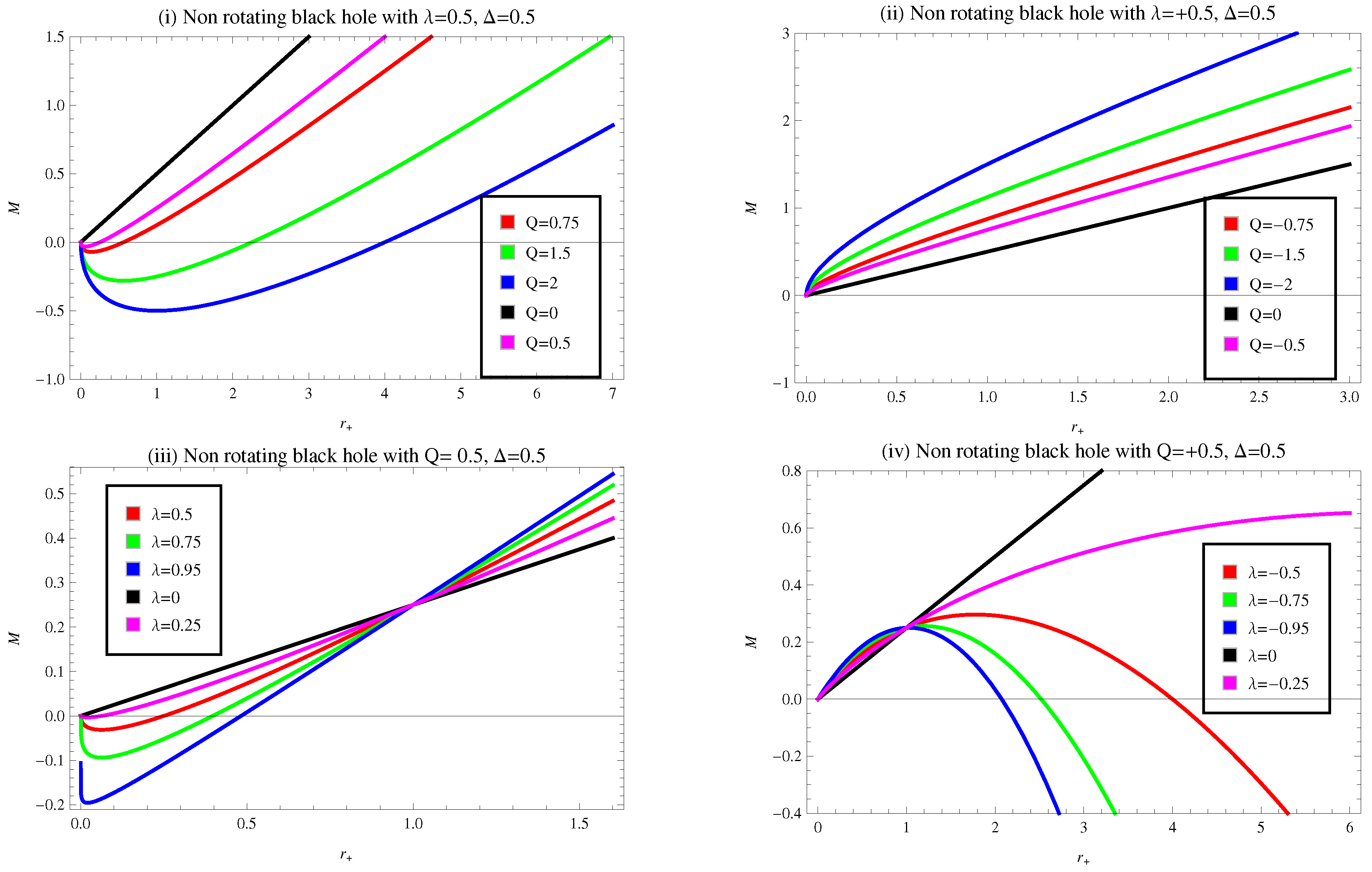
3.1. Mass
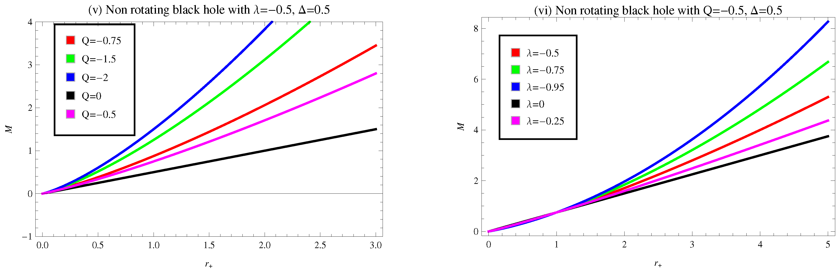
3.2. Temperature
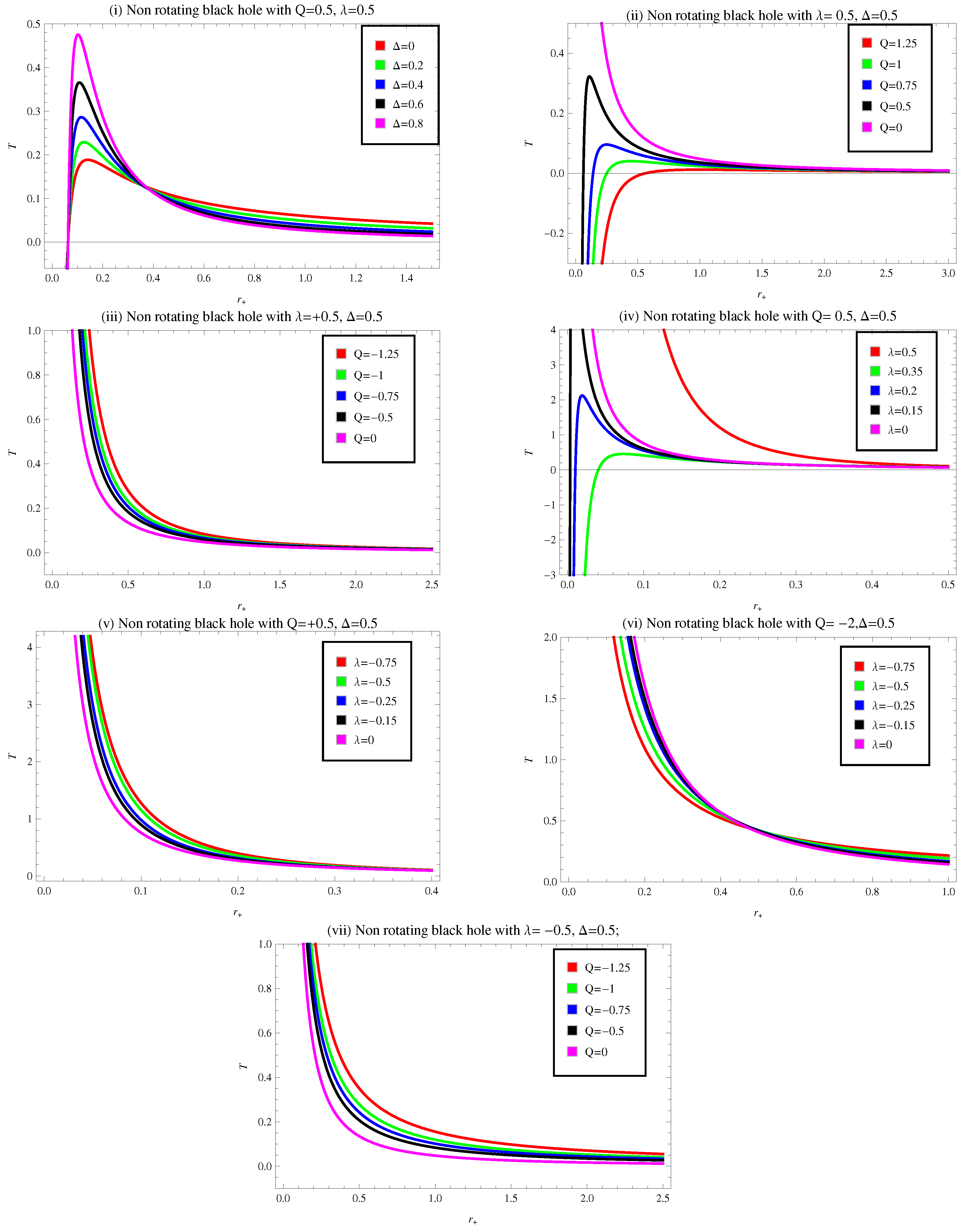
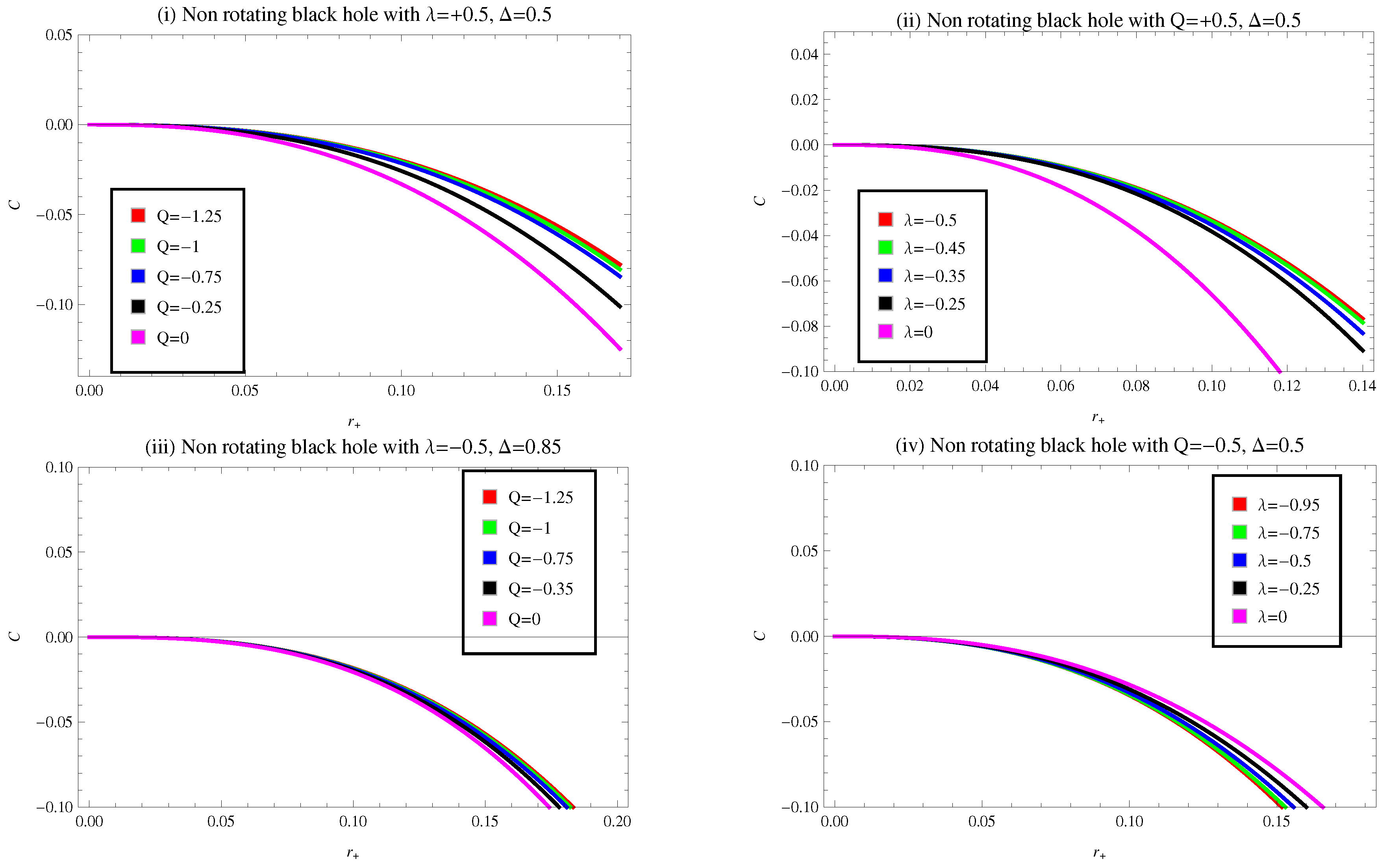
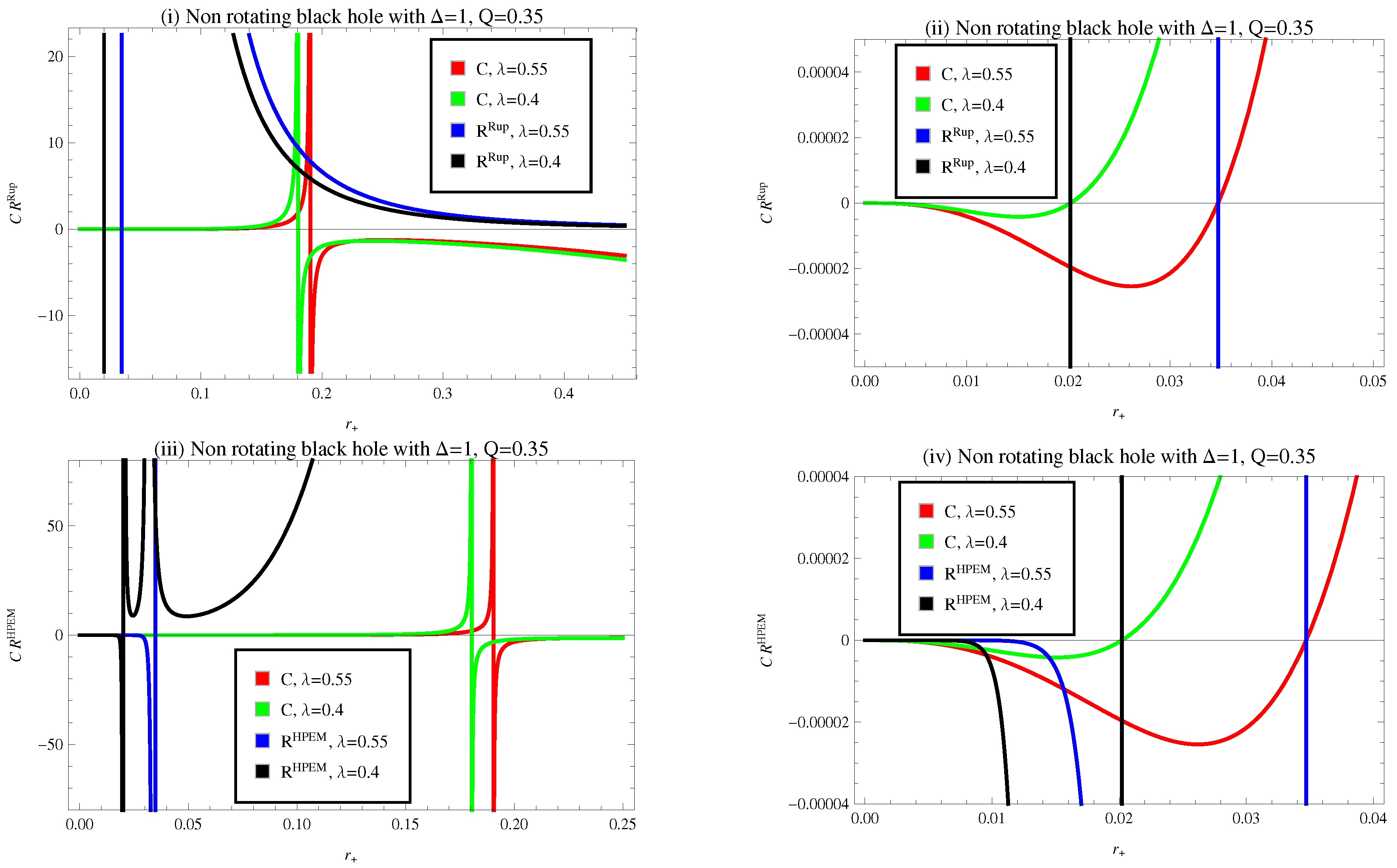
3.3. Heat Capacity
4. Thermodynamic Geometries
5. Rotating Regular Black Hole in Conformal Massive Gravity
6. Thermodynamic Properties
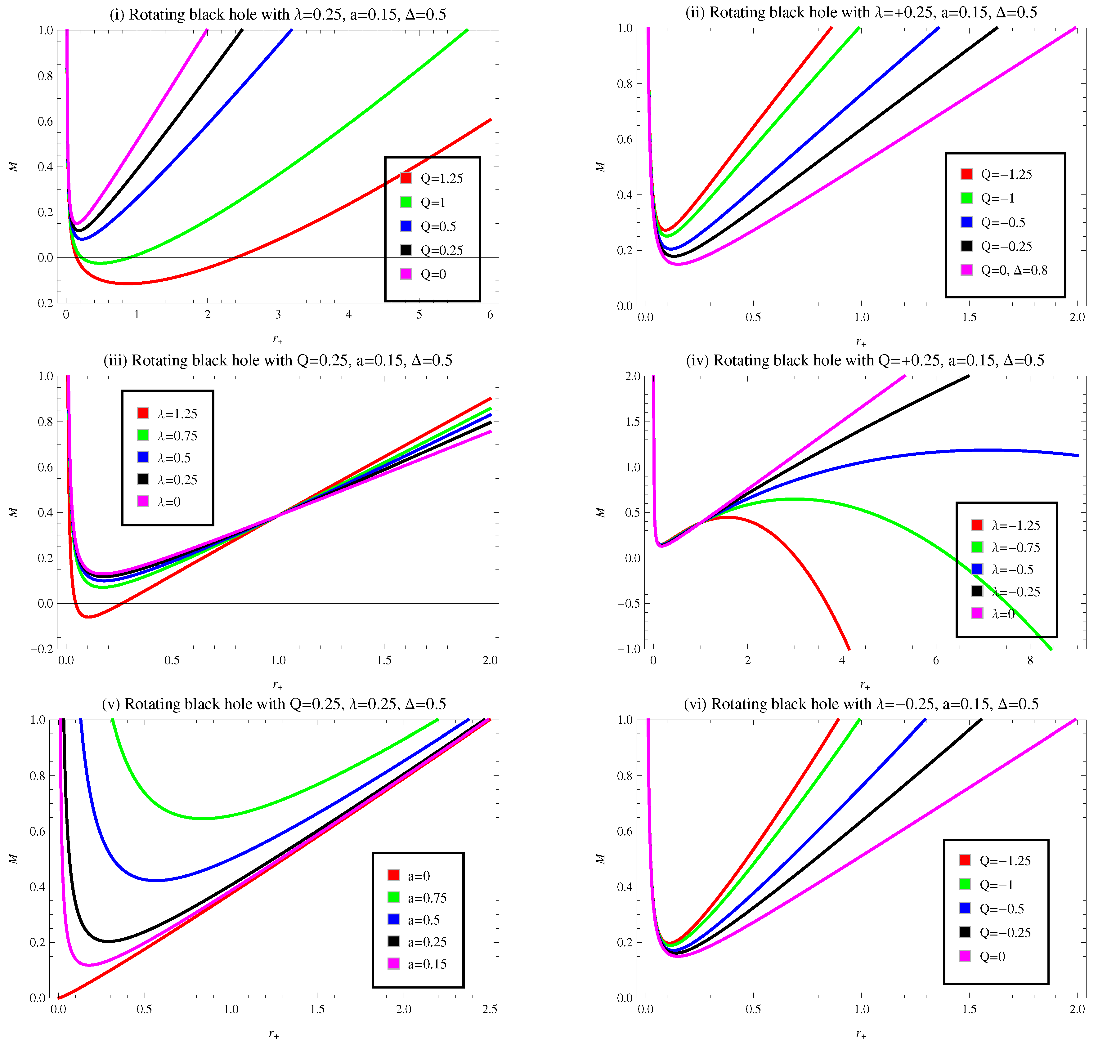
6.1. Mass
6.2. Temperature
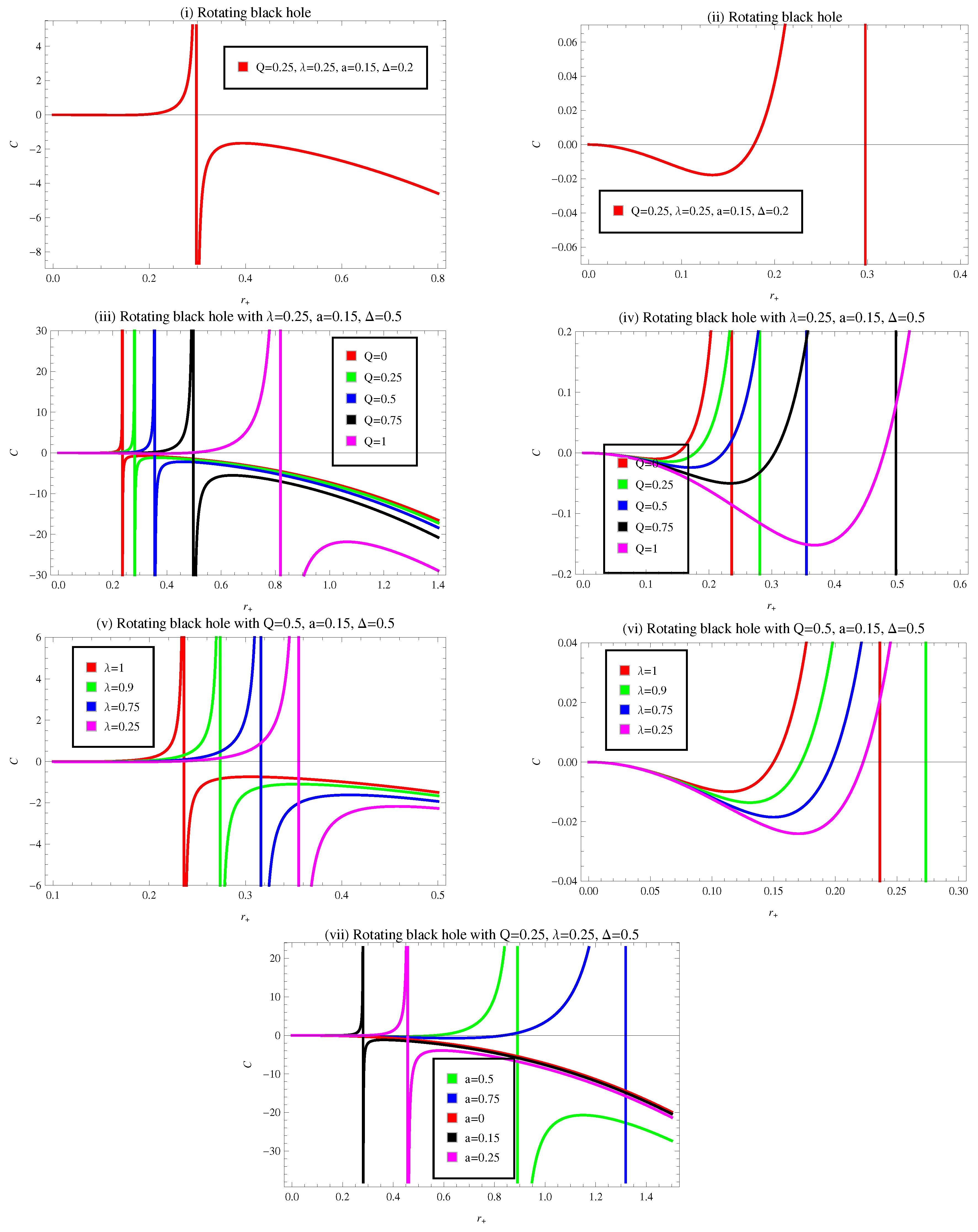
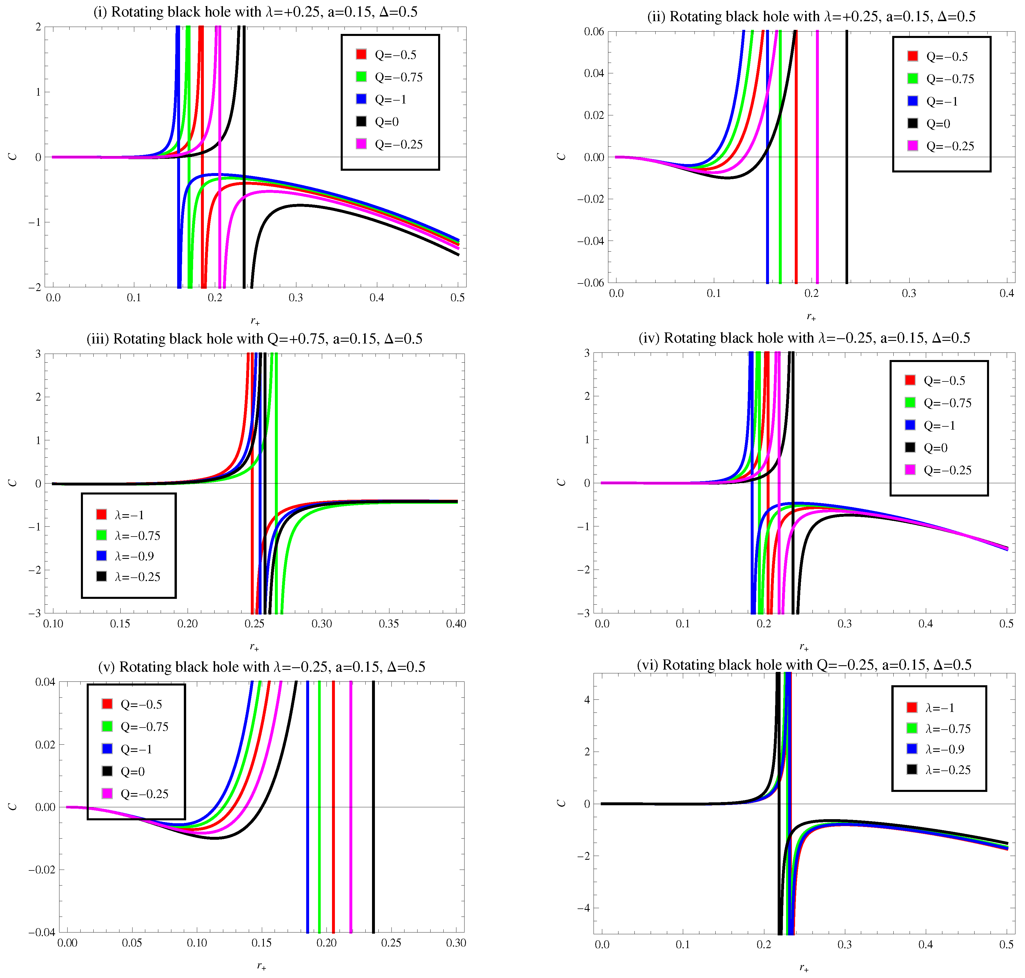
6.3. Heat Capacity
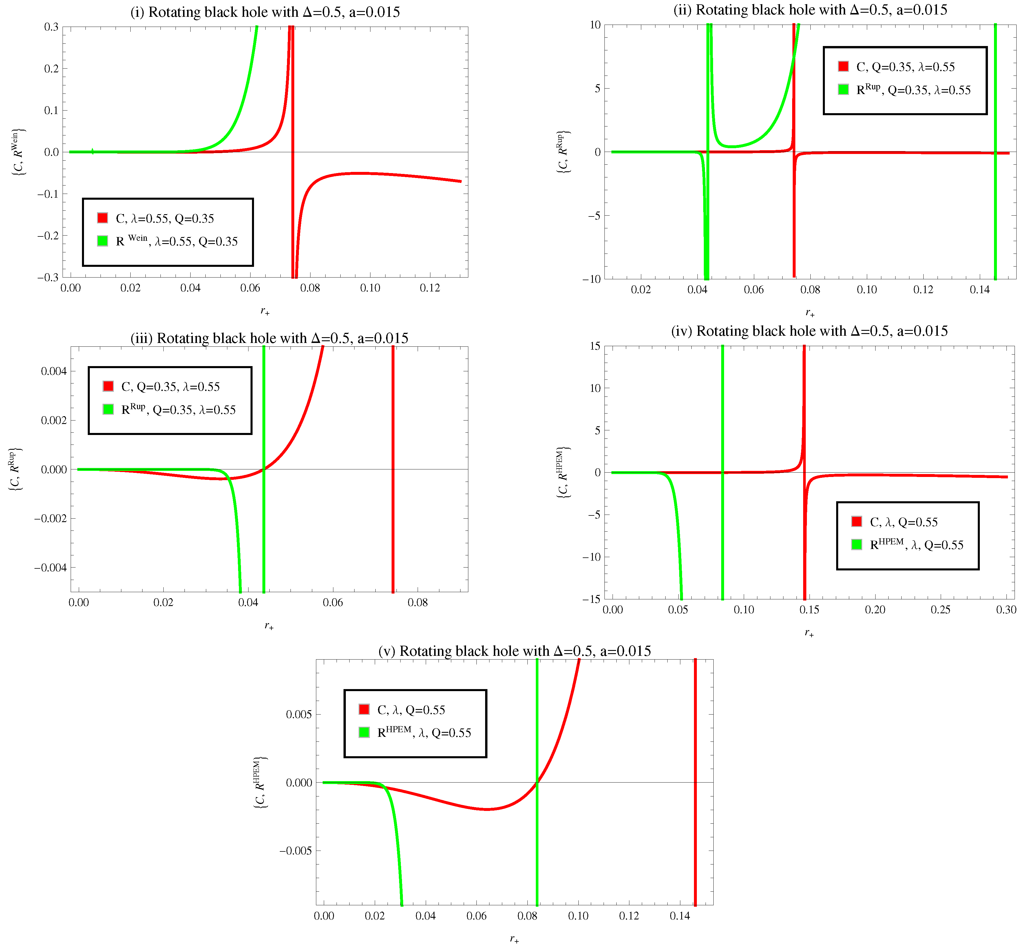
7. Thermodynamic Geometries for Rotating Black Hole
8. Concluding Remarks
Author Contributions
Funding
Data Availability Statement
Conflicts of Interest
References
- Barish, B.C.; Weiss, R. LIGO and the detection of gravitational waves. Phys. Today 1999, 52, 44. [Google Scholar] [CrossRef]
- Akiyama, K.; Alberdi, A.; Alef, W.; Asada, K.; Azulay, R.; Baczko, A.K.; Ball, D.; Baloković, M.; Barrett, J.; Bintley, D. First M87 event horizon telescope results. VI. The shadow and mass of the central black hole. Astrophys. J. Lett. 2019, 875, L6. [Google Scholar]
- Einstein, A. Die Feldgleichungen der Gravitation, Sitzung der Physikalische-Mathematischen Klasse; Scientific Research: Atlanta, GA, USA, 1915; Volume 25, pp. 844–847. [Google Scholar]
- Einstein, A. Die Grundlage der Allgemeinen Relativitätstheorie; Wiley Online library: Hoboken, NJ, USA, 1916; Volume 49, pp. 769–822. [Google Scholar]
- Bel, L. Über das gravitationsfeld eines massenpunktes nach der Einsteinschen theorie. arXiv 2007, arXiv:0709.2257. [Google Scholar]
- Droste, J. The Field of a Single Centre in Einstein’s Theory of Gravitation, and the Motion of a Particle in That Field, Koninklijke Nederlandsche Akademie van Wetenschappen; KNAW: Amsterdam, The Netherlands, 1917; Volume 19, pp. 197–215. [Google Scholar]
- Reissner, H. Über die Eigengravitation des Elektrischen Feldes Nach der Einstein’schen Theorie, Annalen der Physik; Wiley Online library: Hoboken, NJ, USA, 1916; Volume 50, pp. 106–120. [Google Scholar]
- Kerr, R.P. Gravitational field of a spinning mass as an example of algebraically special metrics. Phys. Rev. Lett. 1963, 111, 237–238. [Google Scholar] [CrossRef]
- Newman, E.T.; Couch, R.; Chinnapared, K.; Exton, A.; Prakash, A.; Torrence, R. Metric of a rotating, charged mass. J. Math. Phys 1965, 6, 918–919. [Google Scholar] [CrossRef]
- Belinskii, V.A.; Khalatnikov, I.M. On the nature of the singularities in the general solution of the gravitational equations. Soviet JETP 1969, 29, 911. [Google Scholar]
- Belinsky, V.A.; Khalatnikov, I.M.; Lifshitz, E.M. Oscillatory approach to a singular point in the relativistic cosmology. Adv. Phys. 1970, 19, 525–573. [Google Scholar] [CrossRef]
- Penrose, R. Gravitational collapse and space-time singularities. Phys. Rev. Lett. 1965, 14, 57–59. [Google Scholar] [CrossRef]
- Hawking, S.W.; Ellis, G.F.R. The Large Scale Structure of Space-Time; Cambridge University Press: Cambridge, UK, 1973. [Google Scholar]
- Ford, L.H. The classical singularity theorems and their quantum loop holes. Int. J. Theor. Phys. 2003, 42, 1219–1227. [Google Scholar] [CrossRef]
- Hawking, S.W.; Penrose, R. The singularities of gravitational collapse and cosmology. Proc. R. Soc. Lond. A 1970, 314, 529–548. [Google Scholar]
- Penrose, R. Golden Oldie: Gravitational collapse: The role of general relativity. Gen. Relativ. Gravit. 2002, 34, 1141–1165. [Google Scholar] [CrossRef]
- Christodoulou, D. The instability of naked singularities in the gravitational collapse of a scalar field. Ann. Math. 1999, 149, 183–217. [Google Scholar] [CrossRef]
- Bekenstein, J.D. Black holes and the second law. Lett. Nuovo C 1972, 4, 737–740. [Google Scholar] [CrossRef]
- Bardeen, J.M.; Carter, B.; Hawking, S.W. The four laws of black hole mechanics. Comm. Math. Phys. 1973, 31, 161–170. [Google Scholar] [CrossRef]
- Hawking, S.W. Black hole explosions. Nature 1974, 248, 30–31. [Google Scholar] [CrossRef]
- Davies, P.C.W. Thermodynamics of black holes. Rep. Prog. Phys. 1978, 41, 1313–1355. [Google Scholar] [CrossRef]
- Cai, R.G. Effective spatial dimension of extremal nondilatonic black p-branes and the description of entropy on the world volume. Phys. Rev. Lett. 1997, 78, 2531–2534. [Google Scholar] [CrossRef]
- Maldacena, J.M. The large N limit of superconformal field theories and supergravity. Int. J. Theor. Phys. 1999, 38, 1133. [Google Scholar] [CrossRef]
- Shen, J.Y.; Cai, R.G.; Wang, B.; Su, R.K. Thermodynamic geometry and critical behavior of black holes. Inter. J. Mod. Phys. A 2007, 22, 11–27. [Google Scholar] [CrossRef]
- Hawking, S.W.; Page, D.N. Thermodynamics of black holes in anti-de Sitter space. Comm. Math. Phys. 1983, 87, 577. [Google Scholar] [CrossRef]
- Witten, E. Anti-de Sitter space, thermal phase transition, and confinement in gauge theories. Adv. Theor. Math. Phys 1998, 2, 505–532. [Google Scholar] [CrossRef]
- Weinhold, F. Metric geometry of equilibrium thermodynamics. J. Chem. Phys. 1975, 63, 2479. [Google Scholar] [CrossRef]
- Weinhold, F. Thermodynamics and geometry. Phys. Today 1976, 29, 23. [Google Scholar] [CrossRef]
- Ruppeiner, G. Thermodynamics: A Riemannian geometric model. Phys. Rev. A 1979, 20, 1608. [Google Scholar] [CrossRef]
- Ruppeiner, G. Riemannian geometry in thermodynamic fluctuation theory. Rev. Mod. Phys. 1995, 67, 605. [Google Scholar] [CrossRef]
- Salamon, P.; Nulton, J.D.; Ihrig, E. On the relation between entropy and energy versions of thermodynamic length. J. Chem. Phys. 1984, 80, 436. [Google Scholar] [CrossRef]
- Salamon, P.; Ihrig, E.; Berry, R.S. A group of coordinate transformations which preserve the metric of weinhold. J. Math. Phys. 1983, 24, 2515. [Google Scholar] [CrossRef]
- Mrugala, R.; Nulton, J.D.; Schön, J.C.; Salomon, P. Contact structure in thermodynamic theory. Rep. Math. Phys. 1991, 29, 109. [Google Scholar] [CrossRef]
- Quevedo, H. Geometrothermodynamics. J. Math. Phys. 2007, 48, 013506. [Google Scholar] [CrossRef]
- Hendi, S.H.; Panahiyan, S.; Panah, B.E.; Momennia, M. A new approach toward geometrical concept of black hole thermodynamics. Eur. Phys. J. C 2015, 75, 1–12. [Google Scholar] [CrossRef]
- Mansoori, S.A.H.; Mirza, B. Correspondence of phase transition points and singularities of thermodynamic geometry of black holes. Eur. Phys. J. C 2014, 74, 2681. [Google Scholar] [CrossRef]
- Azreg-Aïnou, M. Geometrothermodynamics: Comments, criticisms, and support. Eur. Phys. J. C 2014, 74, 2930. [Google Scholar] [CrossRef]
- Mansoori, S.A.H.; Mirza, B. Geometrothermodynamics as a singular conformal thermodynamic geometry. Phys. Lett. B 2019, 799, 135040. [Google Scholar] [CrossRef]
- Ebrahimi, K.M.; Mirza, B.; Kachi, M.T. Thermodynamic geometry of pure Lovelock black holes. Int. J. Mod. Phys. D 2022, 13, 2250097. [Google Scholar]
- Zhang, C.Y.; Liu, P.; Liu, Y.; Niu, C.; Wang, B. Dynamical scalarization in Einstein-Maxwell-dilaton theory. Phys. Rev. D 2022, 105, 024073. [Google Scholar] [CrossRef]
- Junior, H.C.D.L.; Yang, J.Z.; Crispino, L.C.B.; Cunha, P.V.P.; Herdeiro, C.A.R. Einstein-Maxwell-dilaton neutral black holes in strong magnetic fields: Topological charge, shadows, and lensing. Phys. Rev. D 2022, 105, 064070. [Google Scholar] [CrossRef]
- Richarte, M.G.; Martins, É.L.; Fabris, J.C. Scattering and absorption of a scalar field impinging on a charged black hole in the Einstein-Maxwell-dilaton theory. Phys. Rev. D 2022, 105, 064043. [Google Scholar] [CrossRef]
- Rogatko, M. Classification of static black holes in Einstein phantom-dilaton Maxwell–anti-Maxwell gravity systems. Phys. Rev. D 2022, 105, 104021. [Google Scholar] [CrossRef]
- Karakasis, T.; Papantonopoulos, E.; Tang, Z.Y.; Wang, B. Rotating (2+1)-dimensional Black Holes in Einstein-Maxwell-Dilaton Theory. arXiv 2022, arXiv:2210.15704. [Google Scholar] [CrossRef]
- Zhang, M.Y.; Chen, H.; Hassanabadi, H.; Long, Z.W.; Yang, H. Joule-Thomson expansion of charged dilatonic black holes. Chin. Phys. C 2022. [Google Scholar] [CrossRef]
- Fernandes, P.G.S. Einstein—Maxwell-scalar black holes with massive and self-interacting scalar hair. Phys. Dark Universe 2020, 30, 100716. [Google Scholar] [CrossRef]
- Bekenstein, J.D. Black holes and entropy. Phys. Rev. D 1973, 7, 2333. [Google Scholar] [CrossRef]
- Hawking, S.W. Particle creation by black holes. Commun. Math. Phys. 1975, 43, 199. [Google Scholar] [CrossRef]
- Barrow, J.D. The area of a rough black hole. Phys. Lett. B 2020, 808, 135643. [Google Scholar] [CrossRef]
- Mamon, A.A.; Paliathanasis, A.; Saha, S. Dynamics of an interacting Barrow holographic dark energy model and its thermodynamic implications. Eur. Phys. J. Plus 2021, 136, 134. [Google Scholar] [CrossRef]
- Adhikary, P.; Das, S.; Basilakos, S.; Saridakis, E.N. Barrow holographic dark energy in a nonflat universe. Phys. Rev. D 2021, 104, 123519. [Google Scholar] [CrossRef]
- Soroushfar, S.; Saffari, R.; Abebe, A.; Sheikhahmadi, H. Thermodynamic geometry of static and rotating regular black holes in conformal massive gravity. Eur. Phys. J. Plus 2021, 136, 1223. [Google Scholar] [CrossRef]
- Bambi, C.; Modesto, L.; Rachwal, L. Spacetime completeness of non-singular black holes in conformal gravity. JCAP 2017, 2017, 3. [Google Scholar] [CrossRef]
- Chakrabarty, H.; Benavides-Gallego, C.A.; Bambi, C.; Modesto, L. Unattainable extended spacetime regions in conformal gravity. J. High Energy Phys. 2018, 2018, 13. [Google Scholar] [CrossRef]
- Jusufi, K.; Jamil, M.; Chakrabarty, H.; Wu, Q.; Bambi, C.; Wang, A. Rotating regular black holes in conformal massive gravity. Phys. Rev. D 2020, 101, 044035. [Google Scholar] [CrossRef]
- Jusufi, K.; Anou, M.A.; Jamil, M.; Saridakis, E.N. Constraints on Barrow entropy from M87* and S2 star observations. Universe 2022, 8, 102. [Google Scholar] [CrossRef]
- Saridakis, E.N. Barrow holographic dark energy. Phys. Rev. D 2020, 102, 123525. [Google Scholar] [CrossRef]
- Saridakis, E.N. Modified cosmology through spacetime thermodynamics and Barrow horizon entropy. JCAP 2020, 2020, 31. [Google Scholar] [CrossRef]
- Abreu, E.M.C.; Neto, J.A. Barrow black hole corrected-entropy model and Tsallis nonextensivity. Phys. Lett. B 2020, 810, 135805. [Google Scholar] [CrossRef]
- Abreu, E.M.C.; Neto, J.A.; Barboza, E.M. Barrow’s black hole entropy and the equipartition theorem. Europhys. Lett. 2020, 130, 40005. [Google Scholar] [CrossRef]
- Kaul, R.K.; Majumdar, P. Logarithmic correction to the Bekenstein-Hawking entropy. Phys. Rev. Lett. 2000, 84, 5255. [Google Scholar] [CrossRef] [PubMed]
- Carlip, S. Logarithmic corrections to black hole entropy, from the Cardy formula. Class. Quantum Gravity 2000, 17, 4175. [Google Scholar] [CrossRef]
- Tsallis, C. Generalized entropy-based criterion for consistent testing. Phys. Rev. E 1988, 58, 1442. [Google Scholar] [CrossRef]
- Tsallis, C.; Cirto, L.J.L. Black hole thermodynamical entropy. Eur. Phys. J. C 2013, 73, 2487. [Google Scholar] [CrossRef]
- Bondi, H. Negative mass in general relativity. Rev. Mod. Phys. 1957, 29, 423. [Google Scholar] [CrossRef]
- Castelvecchi, D. Artificial black hole creates its own version of Hawking radiation. Nature 2016, 536, 7616. [Google Scholar] [CrossRef] [PubMed]
- Khamehchi, M.A.; Hossain, K.; Mossman, M.E.; Zhang, Y.; Busch, T.; Forbes, M.M.; Engels, P. Negative-mass hydrodynamics in a spin-orbit-coupled Bose-Einstein condensate. Phys. Rev. Lett. 2017, 118, 155301. [Google Scholar] [CrossRef] [PubMed]
- Farnes, V. A unifying theory of dark energy and dark matter: Negative masses and matter creation within a modified ΛCDM framework. Astron. Astrophys. 2018, 620, A92. [Google Scholar] [CrossRef]
- Pacilio, C. Scalar charge of black holes in Einstein-Maxwell-dilaton theory. Phys. Rev. D 2018, 98, 064055. [Google Scholar] [CrossRef]
- Salamon, P.; Nulton, J.D.; Ihrig, E. Thermodynamic lengths and intrinsic time scales in molecular relaxation. J. Chem. Phys. 1984, 80, 436. [Google Scholar] [CrossRef]
- Mrugala, R. On equivalence of two metrics in classical thermodynamics. Phys. A Stat. Mech. App. 1984, 125, 631. [Google Scholar] [CrossRef]
- Hendi, S.H.; Sheykhi, A.; Panahiyan, S.; Panah, B.E. Phase transition and thermodynamic geometry of Einstein-Maxwell-dilaton black holes. Phys. Rev. D 2015, 92, 064028. [Google Scholar] [CrossRef]
- Soroushfar, S.; Saffari, R.; Upadhyay, S. Thermodynamic geometry of a black hole surrounded by perfect fluid in Rastall theory. Gen. Relativ. Gravit. 2019, 51, 130. [Google Scholar] [CrossRef]
- Quevedo, H. Geometrothermodynamics of black holes. Gen. Relativ. Gravit. 2008, 40, 971. [Google Scholar] [CrossRef]
- Quevedo, H.; Sanchez, A. Geometric description of BTZ black holes thermodynamics. Phys. Rev. D 2009, 79, 024012. [Google Scholar] [CrossRef]
- Quevedo, H.; Quevedo, M.N.; Sanchez, A. Geometrothermodynamics of phantom AdS black holes. Eur. Phys. J. C 2016, 76, 110. [Google Scholar] [CrossRef]
- Hermann, R. Geometry, Physics and Systems; Marcel Dekker: New York, NY, USA, 1973. [Google Scholar]
- Mrugala, R. Geometrical formulation of equilibrium phenomenological thermodynamics. Rep. Math. Phys. 1978, 14, 419. [Google Scholar] [CrossRef]
- Mrugala, R. Submanifolds in the thermodynamic phase space. Rep. Math. Phys. 1985, 21, 197. [Google Scholar] [CrossRef]
- Azreg-Aïnou, M. Generating rotating regular black hole solutions without complexification. Phys. Rev. D 2014, 90, 064041. [Google Scholar] [CrossRef]
- Soroushfar, S.; Upadhyay, S. Phase transition of a charged AdS black hole with a global monopole through geometrical thermodynamics. Phys. Lett. B 2020, 804, 135360. [Google Scholar] [CrossRef]
- Pourhassan, B.; Wani, S.S.; Soroushfar, S.; Faizal, M. Quantum work and information geometry of a quantum Myers-Perry black hole. J. High Energy Phys. 2021, 2021, 1–27. [Google Scholar] [CrossRef]

Disclaimer/Publisher’s Note: The statements, opinions and data contained in all publications are solely those of the individual author(s) and contributor(s) and not of MDPI and/or the editor(s). MDPI and/or the editor(s) disclaim responsibility for any injury to people or property resulting from any ideas, methods, instructions or products referred to in the content. |
© 2023 by the authors. Licensee MDPI, Basel, Switzerland. This article is an open access article distributed under the terms and conditions of the Creative Commons Attribution (CC BY) license (https://creativecommons.org/licenses/by/4.0/).
Share and Cite
Jawad, A.; Hussain, M.; Rani, S. Applications of Thermodynamic Geometries to Conformal Regular Black Holes: A Comparative Study. Universe 2023, 9, 87. https://doi.org/10.3390/universe9020087
Jawad A, Hussain M, Rani S. Applications of Thermodynamic Geometries to Conformal Regular Black Holes: A Comparative Study. Universe. 2023; 9(2):87. https://doi.org/10.3390/universe9020087
Chicago/Turabian StyleJawad, Abdul, Mazhar Hussain, and Shamaila Rani. 2023. "Applications of Thermodynamic Geometries to Conformal Regular Black Holes: A Comparative Study" Universe 9, no. 2: 87. https://doi.org/10.3390/universe9020087
APA StyleJawad, A., Hussain, M., & Rani, S. (2023). Applications of Thermodynamic Geometries to Conformal Regular Black Holes: A Comparative Study. Universe, 9(2), 87. https://doi.org/10.3390/universe9020087