
Release Episodes of Electrons and Protons in Solar Energetic Particle Events

 ,
,  , , and
Abstract
:1. Introduction
2. Data Selection and Analysis Methods
2.1. Data Selection
2.2. Data Analysis and Methods
2.2.1. Onset Time Determination
2.2.2. Velocity Dispersion Analysis
2.2.3. Fraction Velocity Dispersion Analysis
2.2.4. Time Shifting Analysis
3. Results
3.1. SEP Associations with Other Observables
3.2. The Classification of SEP Events
3.3. Analysis
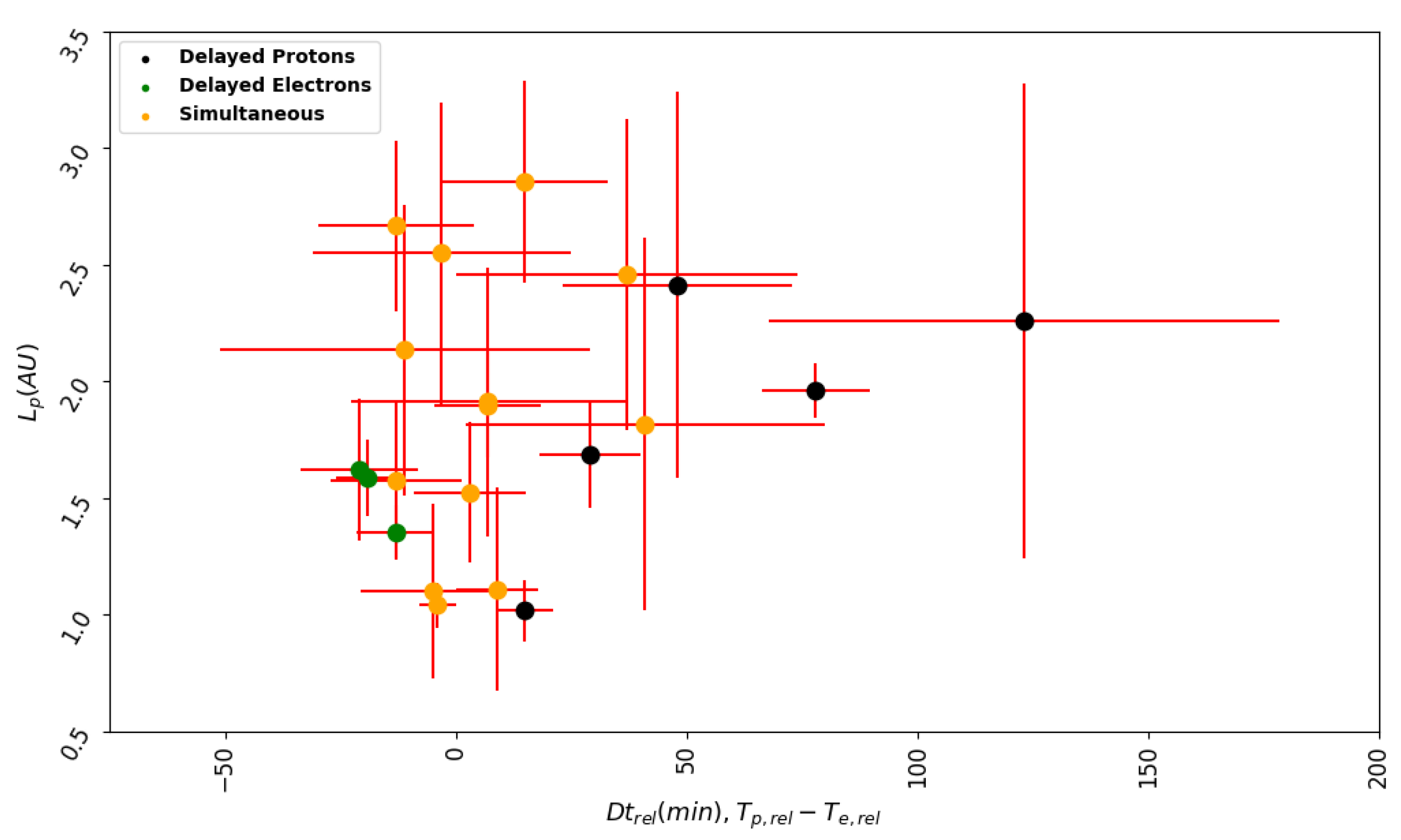
3.3.1. Path Lengths for Protons and Electrons:
3.3.2. Proton Event Groups
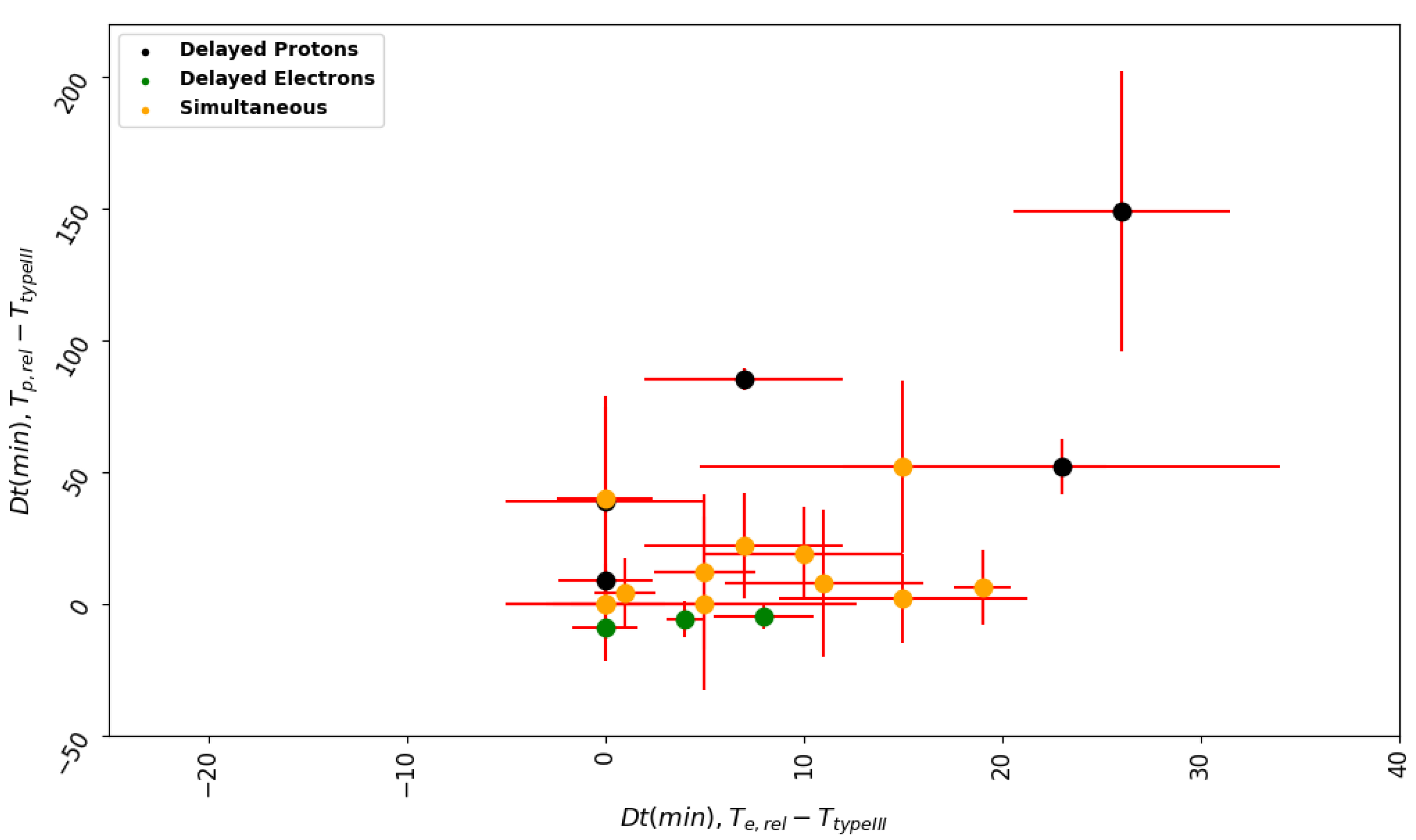
3.3.3. Proton Events, Temporarily Related Electron Events, and Release Episodes
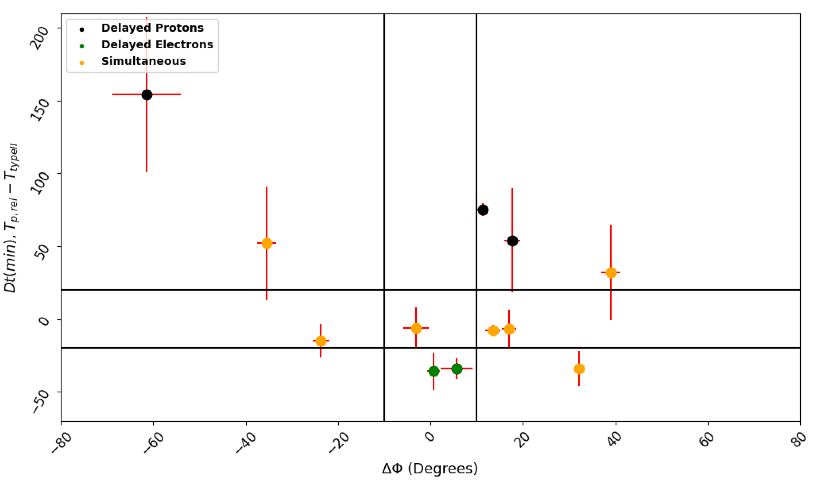
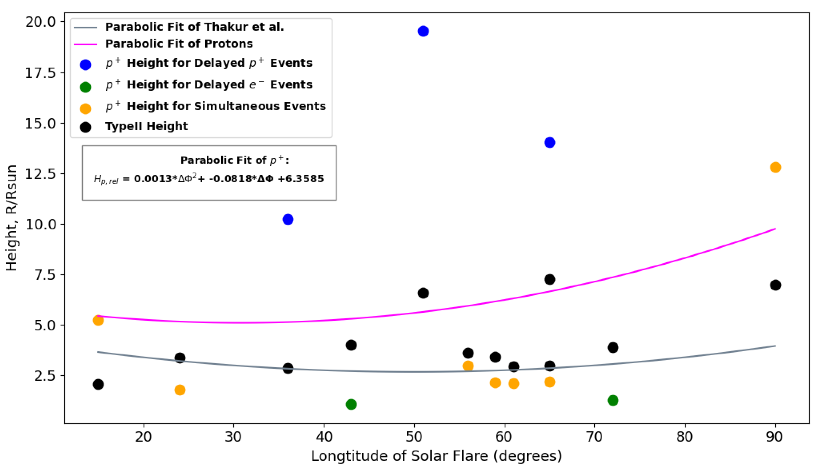
3.3.4. Release Episodes and the Location of the Solar Source
3.3.5. Release Episodes and Shock Heights
4. Discussion & Conclusions
Author Contributions
Funding
Data Availability Statement
Acknowledgments
Conflicts of Interest
Appendix A. The 21 SEP Events of the Study

| ID | Event Date | T | T (min) | T | T (min) | H | T | T | T | H | (°) | (°) | |
|---|---|---|---|---|---|---|---|---|---|---|---|---|---|
| 1 | 9 May1999 | 18:00 | 33 | 18:11 | 7.66 | 2.76 | 3.34 | 17:54 | 18:06 | Nan | Nan | Nan | Nan |
| 2 | 27 May 1999 | 11:14 | 6.14 | 10:59 | 2.39 | 5.99 | 3.8 | 10:36 | 11:05 | 10:55 | 3.22 | Nan | Nan |
| 3 | 11 June 1999 | 0:35 | 4.53 | 0:48 | 2.52 | 1.8 | 2.61 | 00:40 | Nan | Nan | Nan | Nan | |
| 4 | 18 February 2000 | 9:10 | 6.95 | 9:29 | 0.93 | 1.27 | 2.73 | 9:16 | 9:25 | 9:44 | 3.88 | 72 | 5.66 |
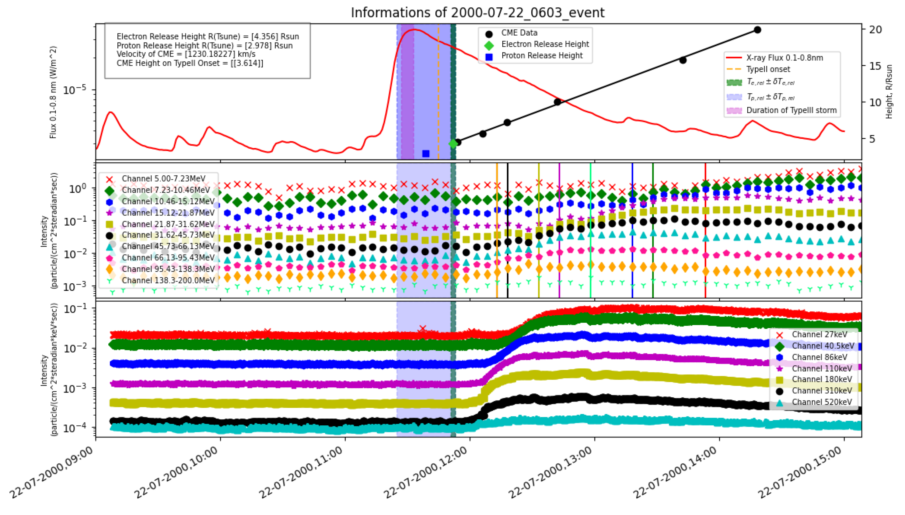
| 5 | 22 July 2000 | 11:39 | 14.15 | 11:52 | 1.41 | 2.98 | 4.36 | 11:27 | 11:33 | 11:45 | 3.61 | 56 | −3.1 |
| 6 | 20 May 2001 | 6:29 | 17.76 | 6:20 | 5 | 3.34 | 2.92 | 06:10 | 6:05 | 2.22 | Nan | Nan | |
| 7 | 4 June 2001 | 16:49 | 29.66 | 16:42 | 2.55 | 4 | 3.72 | 16:22 | 16:37 | Nan | Nan | 59 | 1.17 |
| 8 | 27 January 2002 | 12:32 | 16.84 | 12:45 | 6.24 | 3.34 | 4.62 | 12:10 | 12:30 | 12:49 | 5.01 | Nan | Nan |
| 9 | 18 August 2002 | 22:12 | 10.56 | 21:43 | 11 | 4.33 | 2.63 | 21:10 | 21:20 | Nan | Nan | 19 | −26.08 |
| 10 | 20 August 2002 | 8:38 | 27.87 | 8:41 | 5 | 3.57 | 3.85 | 8:25 | 8:30 | Nan | Nan | 38 | −13.99 |
| 11 | 31 May 2003 | 2:28 | 11.99 | 2:33 | 5 | 2.2 | 2.99 | 2:20 | 2:40 | 3:00 | 7.26 | 65 | 32.13 |
| 12 | 9 November 2004 | 18:50 | 4.3 | 17:32 | 5 | 19.53 | 6.08 | 17:00 | 17:25 | 17:35 | 6.6 | 51 | 11.32 |
| 13 | 14 July 2005 | 11:32 | 32.58 | 10:55 | 10.25 | 12.81 | 6.07 | 10:20 | 10:40 | 11:00 | 6.98 | 90 | 39.05 |
| 14 | 22 August 2005 | 18:09 | 35.71 | 17:21 | 5 | 14.04 | 4.2 | 17:00 | 17:30 | 17:15 | 2.97 | 65 | 17.74 |
| 15 | 21 March 2011 | 2:57 | 20.08 | 2:42 | 5 | 6.05 | 4.31 | 2:17 | 2:35 | 2:20 | 1.77 | Nan | Nan |
| 16 | 2 August 2011 | 7:07 | 38.96 | 6:26 | 2.42 | 5.24 | 2.73 | 6:03 | 6:27 | 6:15 | 2.05 | 15 | −35.44 |
| 17 | 8 August 2011 | 18:03 | 13.03 | 18:00 | 1.53 | 2.12 | 1.77 | 17:59 | 18:10 | 2.93 | 61 | 17.08 | |
| 18 | 13 March 2012 | 17:27 | 3.98 | 17:31 | 1.75 | 2.13 | 2.78 | 17:20 | 17:42 | 17:35 | 3.43 | 59 | 13.51 |
| 19 | 20 February 2014 | 7:29 | 12.73 | 7:50 | 1.62 | 1.06 | 2.78 | 7:38 | 7:51 | 8:05 | 4 | 43 | 0.69 |
| 20 | 25 August 2014 | 17:54 | 53.17 | 15:51 | 5.46 | 10.25 | 4.36 | 14:50 | 15:25 | 15:20 | 2.88 | 36 | −61.41 |
| 21 | 20 September 2015 | 18:08 | 11.55 | 18:01 | 3 | 1.78 | 1.03 | 17:55 | 18:20 | 18:23 | 3.39 | 24 | −23.7 |
| No | Date | Proton VDA | Electron FVDA | Electron TSA | SXR | CME (1st obs.) | ||||
|---|---|---|---|---|---|---|---|---|---|---|
| UT | (AU) | UT | (AU) | UT | (Peak Time) | (Magnitude) | (°) | UT | ||
| 1 | 9 May 1999 | 18:00 ± 33 | 2.13 ± 0.62 | 18:11 ± 08 | 1.76 ± 0.40 | 18:10 ± 05 | 18:10 | M7.6 | Nan (long > 90) | 18:28 |
| 2 | 27 May 1999 | 11:14 ± 06 | 1.02 ± 0.13 | 10:59 ± 02 | 1.20 ± 0.13 | 10:57 ± 05 | Nan | Nan | Nan | 11:06 |
| 3 | 11 June 1999 | 00:35 ± 05 | 1.35 ± 0.12 | 00:48 ± 03 | 1.62 ± 0.13 | 00:47 ± 05 | Nan | Nan | Nan | 01:27 |
| 4 | 18 February 2000 | 09:10 ± 06 | 1.59 ± 0.17 | 09:29 ± 01 | 1.13 ± 0.05 | 09:21 ± 05 | 09:23 | C1.1 | 72W | 09:54 |
| 5 | 22 July 2000 | 11:39 ± 14 | 1.58 ± 0.34 | 11:52 ± 01 | 1.56 ± 0.08 | 11:43 ± 05 | 11:25 | M3.7 | 56W | 11:54 |
| 6 | 20 May 2001 | 06:29 ± 18 | 1.11 ± 0.44 | 06:20 ± 01 | 1.16 ± 0.04 | 06:17 ± 05 | 06:30 | M6.4 | Nan (long > 90) | 06:26 |
| 7 | 4 June 2001 | 16:49 ± 30 | 1.91 ± 0.58 | 16:42 ± 03 | 1.22 ± 0.15 | 16:28 ± 05 | 16:26 | M3.2 | 59W | 16:30 |
| 8 | 27 January 2002 | 12:32 ± 17 | 2.67 ± 0.36 | 12:45 ± 06 | 1.23 ± 0.31 | 12:50 ± 05 | Nan | Nan | Nan | 12:30 |
| 9 | 18 August 2002 | 22:12 ± 11 | 1.69 ± 0.23 | 21:43 ± 11 | 1.22 ± 0.54 | 21:22 ± 05 | 21:36 | M2.2 | 19W | 21:54 |
| 10 | 20 August 2002 | 08:38 ± 28 | 2.55 ± 0.65 | 08:41 ± 08 | 1.12 ± 0.54 | 08:38 ± 05 | 08:24 | M3.4 | 38W | 08:55 |
| 11 | 31 May 2003 | 02:28 ± 12 | 1.10 ± 0.37 | 02:33 ± 02 | 1.05 ± 0.12 | 02:28 ± 05 | 02:21 | M9.3 | 65W | 02:30 |
| 12 | 9 November 2004 | 18:50 ± 4 | 1.96 ± 0.12 | 17:32 ± 14 | 1.07 ± 0.84 | 17:27 ± 05 | 17:13 | M8.9 | 51W | 17:26 |
| 13 | 14 July 2005 | 11:32 ± 32 | 2.46 ± 0.67 | 10:55 ± 10 | 1.72 ± 0.60 | 08:36 ± 05 | 10:21 | X1.2 | 90W | 10:54 |
| 14 | 22 August 2005 | 18:09 ± 36 | 2.41 ± 0.83 | 17:21 ± 01 | 1.10 ± 0.04 | 17:18 ± 05 | 16:57 | M5.6 | 65W | 17:30 |
| 15 | 21 March 2011 | 02:57 ± 20 | 2.86 ± 0.43 | 02:42 ± 11 | 1.12 ± 0.63 | 03:02 ± 05 | Nan | Nan | Nan | 02:24 |
| 16 | 2 August 2011 | 07:07 ± 39 | 1.82 ± 0.80 | 06:26 ± 02 | 1.00 ± 0.14 | 06:23 ± 05 | 06:14 | M1.4 | 15W | 06:36 |
| 17 | 8 August 2011 | 18:03 ± 13 | 1.52 ± 0.30 | 18:00 ± 02 | 1.69 ± 0.08 | 17:59 ± 05 | 18:06 | M3.5 | 61W | 18:12 |
| 18 | 13 March 2012 | 17:27 ± 4 | 1.04 ± 0.09 | 17:31 ± 02 | 1.30 ± 0.10 | 17:29 ± 05 | 17:24 | M7.9 | 59W | 17:36 |
| 19 | 20 February 2014 | 07:29 ± 13 | 1.62 ± 0.30 | 07:50 ± 02 | 1.22 ± 0.08 | 07:49 ± 05 | 07:46 | M3.0 | 43W | 08:00 |
| 20 | 25 August 2014 | 17:54 ± 53 | 2.26 ± 1.02 | 15:51 ± 05 | 1.32 ± 0.33 | 16:08 ± 05 | 15:02 | M2.0 | 36W | 15:36 |
| 21 | 20 September 2015 | 18:08 ± 12 | 1.90 ± 0.22 | 18:01 ± 03 | 1.36 ± 0.17 | 17:47 ± 05 | 17:51 | M2.1 | 24W | 18:12 |
| 1 | https://omniweb.gsfc.nasa.gov/, accessed on 20 September 2023 |
| 2 | https://cdaw.gsfc.nasa.gov/CME_list/, accessed on 20 September 2023 |
| 3 | http://193.190.230.139/, accessed on 20 September 2023 |
| 4 | https://cdaw.gsfc.nasa.gov/CME_list/radio/waves_type2.html, accessed on 20 September 2023 |
| 5 | available at https://secchirh.obspm.fr/, accessed on 20 September 2023 |
| 6 | which follows from the histograms and in the next section |
References
- Desai, M.; Giacalone, J. Large gradual solar energetic particle events. Living Rev. Sol. Phys. 2016, 13, 3. [Google Scholar] [CrossRef] [PubMed]
- Reames, D.V. Solar Energetic Particles: A Modern Primer on Understanding Sources, Acceleration and Propagation; Springer: Berlin/Heidelberg, Germany, 2021. [Google Scholar]
- Carley, E.P.; Vilmer, N.; Vourlidas, A. Radio observations of coronal mass ejection initiation and development in the low solar corona. Front. Astron. Space Sci. 2020, 7, 79. [Google Scholar] [CrossRef]
- Cane, H.V.; Richardson, I.G.; von Rosenvinge, T.T. A study of solar energetic particle events of 1997–2006: Their composition and associations. J. Geophys. Res. (Space Phys.) 2010, 115, A08101. [Google Scholar] [CrossRef]
- Papaioannou, A.; Sandberg, I.; Anastasiadis, A.; Kouloumvakos, A.; Georgoulis, M.K.; Tziotziou, K.; Tsiropoula, G.; Jiggens, P.; Hilgers, A. Solar flares, coronal mass ejections and solar energetic particle event characteristics. J. Space Weather Space Clim. 2016, 6, A42. [Google Scholar] [CrossRef]
- Klein, K.L.; Dalla, S. Acceleration and Propagation of Solar Energetic Particles. Space Sci. Rev. 2017, 212, 1107–1136. [Google Scholar] [CrossRef]
- Kahler, S.W. The role of the big flare syndrome in correlations of solar energetic proton fluxes and associated microwave burst parameters. J. Geophys. Res. Space Phys. 1982, 87, 3439–3448. [Google Scholar] [CrossRef]
- Trottet, G.; Samwel, S.; Klein, K.L.; Dudok de Wit, T.; Miteva, R. Statistical Evidence for Contributions of Flares and Coronal Mass Ejections to Major Solar Energetic Particle Events. Sol. Phys. 2015, 290, 819–839. [Google Scholar] [CrossRef]
- Lavasa, E.; Giannopoulos, G.; Papaioannou, A.; Anastasiadis, A.; Daglis, I.A.; Aran, A.; Pacheco, D.; Sanahuja, B. Assessing the Predictability of Solar Energetic Particles with the Use of Machine Learning Techniques. Sol. Phys. 2021, 296, 107. [Google Scholar] [CrossRef]
- Dierckxsens, M.; Tziotziou, K.; Dalla, S.; Patsou, I.; Marsh, M.S.; Crosby, N.B.; Malandraki, O.; Tsiropoula, G. Relationship between Solar Energetic Particles and Properties of Flares and CMEs: Statistical Analysis of Solar Cycle 23 Events. Sol. Phys. 2015, 290, 841–874. [Google Scholar] [CrossRef]
- Kocharov, L.; Omodei, N.; Mishev, A.; Pesce-Rollins, M.; Longo, F.; Yu, S.; Gary, D.E.; Vainio, R.; Usoskin, I. Multiple Sources of Solar High-energy Protons. Astrophys. J. 2021, 915, 12. [Google Scholar] [CrossRef]
- Reid, H.A.S. A review of recent type III imaging spectroscopy. Front. Astron. Space Sci. 2020, 7, 56. [Google Scholar] [CrossRef]
- Klein, K.L. Radio astronomical tools for the study of solar energetic particles I. Correlations and diagnostics of impulsive acceleration and particle propagation. Front. Astron. Space Sci. 2021, 7, 105. [Google Scholar] [CrossRef]
- Klein, K.L. Radio astronomical tools for the study of solar energetic particles II.Time-extended acceleration at subrelativistic and relativistic energies. Front. Astron. Space Sci. 2021, 7, 93. [Google Scholar] [CrossRef]
- Cliver, E.W.; Kahler, S.W.; Reames, D.V. Coronal Shocks and Solar Energetic Proton Events. Astrophys. J. 2004, 605, 902–910. [Google Scholar] [CrossRef]
- Gopalswamy, N. Solar and geospace connections of energetic particle events. Geophys. Res. Lett. 2003, 30, 8013. [Google Scholar] [CrossRef]
- Gopalswamy, N.; Aguilar-Rodriguez, E.; Yashiro, S.; Nunes, S.; Kaiser, M.L.; Howard, R.A. Type II radio bursts and energetic solar eruptions. J. Geophys. Res. (Space Phys.) 2005, 110, A12S07. [Google Scholar] [CrossRef]
- Papaioannou, A.; Kouloumvakos, A.; Mishev, A.; Vainio, R.; Usoskin, I.; Herbst, K.; Rouillard, A.P.; Anastasiadis, A.; Gieseler, J.; Wimmer-Schweingruber, R.; et al. The first ground-level enhancement of solar cycle 25 on 28 October 2021. Astron. Astrophys. 2022, 660, L5. [Google Scholar] [CrossRef]
- Kouloumvakos, A.; Nindos, A.; Valtonen, E.; Alissandrakis, C.; Malandraki, O.; Tsitsipis, P.; Kontogeorgos, A.; Moussas, X.; Hillaris, A. Properties of solar energetic particle events inferred from their associated radio emission. Astron. Astrophys. 2015, 580, A80. [Google Scholar] [CrossRef]
- Krucker, S.; Lin, R. Two classes of solar proton events derived from onset time analysis. Astrophys. J. 2000, 542, L61. [Google Scholar] [CrossRef]
- Lin, R.P.; Anderson, K.A.; Ashford, S.; Carlson, C.; Curtis, D.; Ergun, R.; Larson, D.; McFadden, J.; McCarthy, M.; Parks, G.K.; et al. A Three-Dimensional Plasma and Energetic Particle Investigation for the Wind Spacecraft. Space Sci. Rev. 1995, 71, 125–153. [Google Scholar] [CrossRef]
- Torsti, J.; Valtonen, E.; Lumme, M.; Peltonen, P.; Eronen, T.; Louhola, M.; Riihonen, E.; Schultz, G.; Teittinen, M.; Ahola, K.; et al. Energetic Particle Experiment ERNE. Sol. Phys. 1995, 162, 505–531. [Google Scholar] [CrossRef]
- Xie, H.; Mäkelä, P.; Gopalswamy, N.; St. Cyr, O. Energy dependence of SEP electron and proton onset times. J. Geophys. Res. Space Phys. 2016, 121, 6168–6183. [Google Scholar] [CrossRef]
- Müller-Mellin, R.; Kunow, H.; Fleißner, V.; Pehlke, E.; Rode, E.; Röschmann, N.; Scharmberg, C.; Sierks, H.; Rusznyak, P.; Mckenna-Lawlor, S.; et al. COSTEP - Comprehensive Suprathermal and Energetic Particle Analyser. Sol. Phys. 1995, 162, 483–504. [Google Scholar] [CrossRef]
- Müller-Mellin, R.; Böttcher, S.; Falenski, J.; Rode, E.; Duvet, L.; Sanderson, T.; Butler, B.; Johlander, B.; Smit, H. The Solar Electron and Proton Telescope for the STEREO Mission. Space Sci. Rev. 2008, 136, 363–389. [Google Scholar] [CrossRef]
- von Rosenvinge, T.T.; Reames, D.V.; Baker, R.; Hawk, J.; Nolan, J.T.; Ryan, L.; Shuman, S.; Wortman, K.A.; Mewaldt, R.A.; Cummings, A.C.; et al. The High Energy Telescope for STEREO. Space Sci. Rev. 2008, 136, 391–435. [Google Scholar] [CrossRef]
- Mewaldt, R.A.; Cohen, C.M.S.; Cook, W.R.; Cummings, A.C.; Davis, A.J.; Geier, S.; Kecman, B.; Klemic, J.; Labrador, A.W.; Leske, R.A.; et al. The Low-Energy Telescope (LET) and SEP Central Electronics for the STEREO Mission. Space Sci. Rev. 2008, 136, 285–362. [Google Scholar] [CrossRef]
- Ameri, D.; Valtonen, E.; Pohjolainen, S. Properties of high-energy solar particle events associated with solar radio emissions. Sol. Phys. 2019, 294, 1–33. [Google Scholar] [CrossRef]
- Paassilta, M.; Raukunen, O.; Vainio, R.; Valtonen, E.; Papaioannou, A.; Siipola, R.; Riihonen, E.; Dierckxsens, M.; Crosby, N.; Malandraki, O.; et al. Catalogue of 55–80 MeV solar proton events extending through solar cycles 23 and 24. J. Space Weather Space Clim. 2017, 7, A14. [Google Scholar] [CrossRef]
- Gold, R.E.; Krimigis, S.M.; Hawkins, S.E., III; Haggerty, D.K.; Lohr, D.A.; Fiore, E.; Armstrong, T.P.; Holland, G.; Lanzerotti, L.J. Electron, Proton, and Alpha Monitor on the Advanced Composition Explorer spacecraft. Space Sci. Rev. 1998, 86, 541–562. [Google Scholar] [CrossRef]
- Stone, E.C.; Frandsen, A.M.; Mewaldt, R.A.; Christian, E.R.; Margolies, D.; Ormes, J.F.; Snow, F. The Advanced Composition Explorer. Space Sci. Rev. 1998, 86, 1–22. [Google Scholar] [CrossRef]
- Crosby, N.; Heynderickx, D.; Jiggens, P.; Aran, A.; Sanahuja, B.; Truscott, P.; Lei, F.; Jacobs, C.; Poedts, S.; Gabriel, S.; et al. SEPEM: A tool for statistical modeling the solar energetic particle environment. Space Weather 2015, 13, 406–426. [Google Scholar] [CrossRef]
- Gopalswamy, N.; Yashiro, S.; Michalek, G.; Xie, H.; Mäkelä, P.; Vourlidas, A.; Howard, R.A. A Catalog of Halo Coronal Mass Ejections from SOHO. Sun Geosph. 2010, 5, 7–16. [Google Scholar]
- Brueckner, G.E.; Howard, R.A.; Koomen, M.J.; Korendyke, C.M.; Michels, D.J.; Moses, J.D.; Socker, D.G.; Dere, K.P.; Lamy, P.L.; Llebaria, A.; et al. The Large Angle Spectroscopic Coronagraph (LASCO). Sol. Phys. 1995, 162, 357–402. [Google Scholar] [CrossRef]
- Miteva, R.; Samwel, S.W.; Krupar, V. Solar energetic particles and radio burst emission. J. Space Weather Space Clim. 2017, 7, A37. [Google Scholar] [CrossRef]
- Gopalswamy, N.; Mäkelä, P.; Yashiro, S. A Catalog of Type II radio bursts observed by Wind/WAVES and their Statistical Properties. Sun Geosph. 2019, 14, 111–121. [Google Scholar] [CrossRef]
- Vainio, R.; Valtonen, E.; Heber, B.; Malandraki, O.E.; Papaioannou, A.; Klein, K.L.; Afanasiev, A.; Agueda, N.; Aurass, H.; Battarbee, M.; et al. The first SEPServer event catalogue~ 68-MeV solar proton events observed at 1 AU in 1996–2010. J. Space Weather Space Clim. 2013, 3, A12. [Google Scholar] [CrossRef]
- Lintunen, J.; Vainio, R. Solar energetic particle event onset as analyzed from simulated data. Astron. Astrophys. 2004, 420, 343–350. [Google Scholar] [CrossRef]
- Tan, L.C.; Malandraki, O.E.; Reames, D.V.; Ng, C.K.; Wang, L.; Patsou, I.; Papaioannou, A. Comparison between path lengths traveled by solar electrons and ions in ground-level enhancement events. Astrophys. J. 2013, 768, 68. [Google Scholar] [CrossRef]
- Kahler, S.; Ragot, B. Near-relativistic electron c/v onset plots. Astrophys. J. 2006, 646, 634. [Google Scholar] [CrossRef]
- Von Rosenvinge, T.; Barbier, L.; Karsch, J.; Liberman, R.; Madden, M.; Nolan, T.; Reames, D.; Ryan, L.; Singh, S.; Trexel, H.; et al. The energetic particles: Acceleration, composition, and transport (EPACT) investigation on the wind spacecraft. Space Sci. Rev. 1995, 71, 155–206. [Google Scholar] [CrossRef]
- Zhao, L.; Li, G.; Zhang, M.; Wang, L.; Moradi, A.; Effenberger, F. Statistical analysis of interplanetary magnetic field path lengths from solar energetic electron events observed by WIND. Astrophys. J. 2019, 878, 107. [Google Scholar] [CrossRef]
- Li, C.; Firoz, K.A.; Sun, L.; Miroshnichenko, L. Electron and proton acceleration during the first ground level enhancement event of solar cycle 24. Astrophys. J. 2013, 770, 34. [Google Scholar] [CrossRef]
- Papaioannou, A.; Souvatzoglou, G.; Paschalis, P.; Gerontidou, M.; Mavromichalaki, H. The First Ground-Level Enhancement of Solar Cycle 24 on 17 May 2012 and Its Real-Time Detection. Sol. Phys. 2014, 289, 423–436. [Google Scholar] [CrossRef]
- Kouloumvakos, A.; Rouillard, A.; Warmuth, A.; Magdalenic, J.; Jebaraj, I.C.; Mann, G.; Vainio, R.; Monstein, C. Coronal Conditions for the Occurrence of Type II Radio Bursts. Astrophys. J. 2021, 913, 99. [Google Scholar] [CrossRef]
- Patsourakos, S.; Vourlidas, A. “Extreme Ultraviolet Waves” are Waves: First Quadrature Observations of an Extreme Ultraviolet Wave from STEREO. Astrophys. J. Lett. 2009, 700, L182–L186. [Google Scholar] [CrossRef]
- Kozarev, K.; Nedal, M.; Miteva, R.; Dechev, M.; Zucca, P. A Multi-Event Study of Early-Stage SEP Acceleration by CME-Driven Shocks—Sun to 1 AU. Front. Astron. Space Sci. 2022, 9, 801429. [Google Scholar] [CrossRef]
- Thakur, N.; Gopalswamy, N.; Xie, H.; Mäkelä, P.; Yashiro, S.; Akiyama, S.; Davila, J. Ground level enhancement in the 2014 January 6 solar energetic particle event. Astrophys. J. Lett. 2014, 790, L13. [Google Scholar] [CrossRef]
- Dresing, N.; Kouloumvakos, A.; Vainio, R.; Rouillard, A. On the Role of Coronal Shocks for Accelerating Solar Energetic Electrons. Astrophys. J. Lett. 2022, 925, L21. [Google Scholar] [CrossRef]
- Cane, H.V.; Lario, D. An Introduction to CMEs and Energetic Particles. Space Sci. Rev. 2006, 123, 45–56. [Google Scholar] [CrossRef]
- Papitashvili, N.; King, J. OMNI Hourly Data, NASA Space Physics Data Facility. 2020. Available online: https://hpde.io/NASA/NumericalData/OMNI/PT1H (accessed on 15 March 2022).


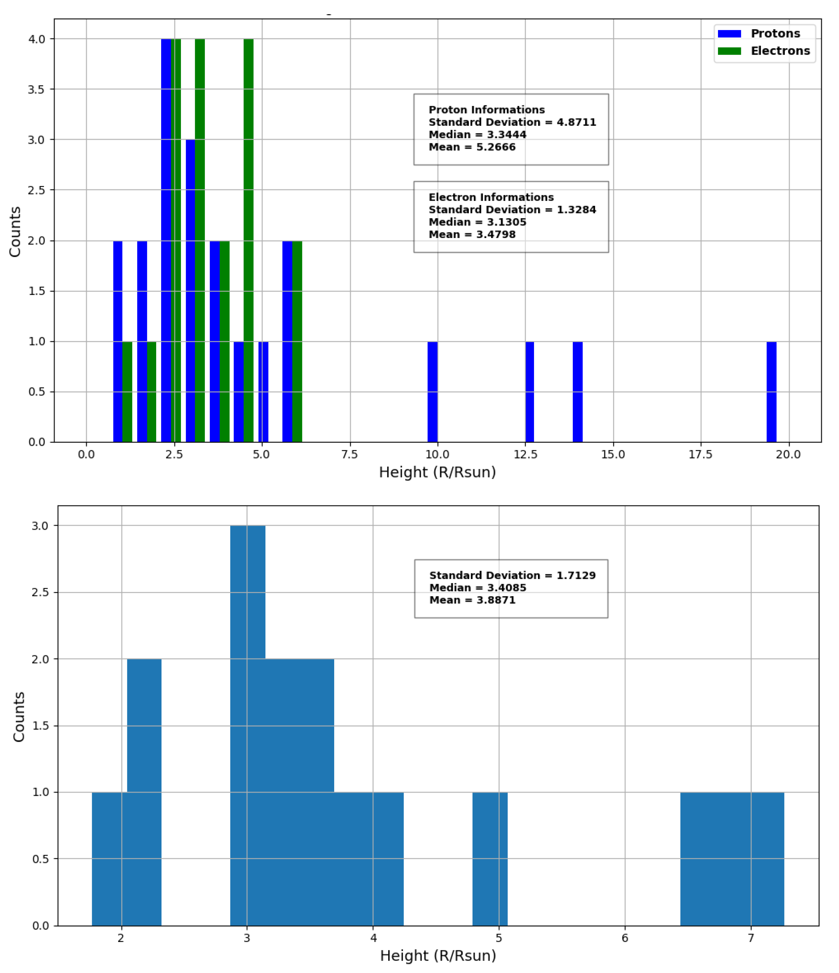
| Mean () | Median () | Standard Deviation () | |
|---|---|---|---|
| 3.48 | 3.13 | 1.33 | |
| 5.27 | 3.44 | 4.87 | |
| 3.89 | 3.41 | 1.71 |
Disclaimer/Publisher’s Note: The statements, opinions and data contained in all publications are solely those of the individual author(s) and contributor(s) and not of MDPI and/or the editor(s). MDPI and/or the editor(s) disclaim responsibility for any injury to people or property resulting from any ideas, methods, instructions or products referred to in the content. |
© 2023 by the authors. Licensee MDPI, Basel, Switzerland. This article is an open access article distributed under the terms and conditions of the Creative Commons Attribution (CC BY) license (https://creativecommons.org/licenses/by/4.0/).
Share and Cite
Kolympiris, V.; Papaioannou, A.; Kouloumvakos, A.; Daglis, I.A.; Anastasiadis, A. Release Episodes of Electrons and Protons in Solar Energetic Particle Events. Universe 2023, 9, 432. https://doi.org/10.3390/universe9100432
Kolympiris V, Papaioannou A, Kouloumvakos A, Daglis IA, Anastasiadis A. Release Episodes of Electrons and Protons in Solar Energetic Particle Events. Universe. 2023; 9(10):432. https://doi.org/10.3390/universe9100432
Chicago/Turabian StyleKolympiris, Vasilis, Athanasios Papaioannou, Athanasios Kouloumvakos, Ioannis A. Daglis, and Anastasios Anastasiadis. 2023. "Release Episodes of Electrons and Protons in Solar Energetic Particle Events" Universe 9, no. 10: 432. https://doi.org/10.3390/universe9100432
APA StyleKolympiris, V., Papaioannou, A., Kouloumvakos, A., Daglis, I. A., & Anastasiadis, A. (2023). Release Episodes of Electrons and Protons in Solar Energetic Particle Events. Universe, 9(10), 432. https://doi.org/10.3390/universe9100432