Abstract
The accelerated expansion of the universe during recent times is well known in cosmology, whereas during early times, there was decelerated expansion. The CDM model is consistent with most observations, but there are some issues with it. In addition, the transition from early deceleration to late-time acceleration cannot be explained by general relativity. Hence, it is worthwhile to examine modified gravity theories to explain this transition and to get a better understanding of dark energy. In this work, dark energy in modified gravity is investigated, where R is the Ricci scalar and T is the trace of the energy momentum tensor. Normally, the simplest form of is used, viz., . In this work, the more complicated form is investigated in Friedmann–Lemaître–Robertson–Walker spacetime. This form has not been well studied. Since the jerk parameter in general relativity is constant and , in order to have as small a departure from general relativity as possible, the jerk parameter is also assumed here. This enables the complete solution for the scale factor to be found. One of these forms is used for a complete analysis and is compared with the usually studied form . The solution can also be broken down into a power-law form at early times (deceleration) and an exponential form at late times (acceleration), which makes the analysis simpler. Surprisingly, each of these forms is also a solution to the differential equation (though they are not solutions to the general solution). The energy conditions are also studied, and plots are provided. It is shown that viable models can be obtained without the need for the introduction of a cosmological constant, which reduces to the CDM at late times.
1. Introduction
It has been a known fact since 1998 that our universe was in a period of slowing expansion in the past but has recently been in a period of accelerated expansion. The information on this accelerated expansion is based on various astrophysical observations [1,2,3,4]. Einstein’s General Relativity (GR) fails to explain this observational late-time accelerated expansion in a natural way. For this reason, it is possible to encounter various attempts and suggestions in the literature to explain this accelerating expansion at the theoretical level. One of the suggestions to complement this deficiency is to associate this late accelerated expansion with an energy of unknown nature called dark energy (DE). What makes the DE concept exotic is the mention here of a negative-pressure, which is interpreted to cause accelerated expansion with an anti-gravity effect. In this context, various DE terms are added to the energy momentum tensor on the right-hand side of Einstein’s field equations, leaving aside the standard cold dark matter (CDM) model in GR [5,6,7,8,9,10,11,12,13].
Alongside the DE concept, modified gravity theories also attempt to explain this accelerated expansion. These theories are mostly constructed by modifying the Ricci scalar curvature R in the Einstein–Hilbert (EH) action on which GR is based. The first thing that comes to mind when changing R is to write an arbitrary function instead of R itself, other curvature terms, or some kind of combination of these. The well-known gravity is one of the best examples of such theories. However, there is no reason why this function f should only be a function of the curvature terms. Modified theories of gravity, including terms related to matter–energy, have also been constructed. The theory of gravity is a modified theory constructed by changing the EH action with a function of both the scalar curvature R and the matter source, which is the trace of the energy–momentum tensor T [14]. In other words, geometry–matter coupling is considered in gravity. In gravity, various universe models have been examined by considering the different forms of the function. However, it would be fair to say that, in general, less attention has been paid to non-minimal coupling forms [15,16,17,18,19].
In this paper, we take into account theory on the background of the flat Friedmann–Lemaître–Robertson–Walker (FLRW) universe for a non-minimal coupling form of the function , i.e., . To solve the field equations, we assume a constant jerk parameter j such that . We give the complete solution for the scale factor to the differential equation for . In addition, this assumption also leads essentially to two different cosmological solutions. One of them corresponds to the past period when the universe expanded by decelerating, and the other corresponds to the late period when it is expanding by accelerating. Both the complete solution and the other solutions separately are investigated in this work. This article is based on an earlier abbreviated paper [19] that appeared in the Proceedings of the 2nd Electronic Online Conference on the Universe held during 16 February–2 March 2023. However, there are several novel aspects in this work, which we shall elucidate upon in the conclusion.
The organization of the article is as follows: In Section 2, the field equations of gravity are given. The field equations for the FLRW metric are given in Section 3, and solutions to the field equations and their consequences are derived in Section 4. The energy conditions are discussed in Section 5, and the conclusion is made in Section 6.
2. Field Equations of Gravity
The field equations of gravity are based on the gravitational action [14]
where is an arbitrary function of the Ricci scalar R and trace T of the energy momentum tensor , g is the determinant of the metric tensor , and is the Lagrangian for the matter. The variation in the gravitational action S in Equation (1) with respect to the metric gives the field equations of gravity as:
Here, is the covariant derivative, is the d’Alembertian operator, and , , with
In the calculation of the variation, the Lagrangian of the matter is taken to depend only on the metric tensor—but not on the derivatives of the metric tensor. Now, we assume that the matter–energy that fills the universe is a perfect fluid. In this case, we can write the energy–momentum tensor of this fluid as follows
Here, and p are the energy density and pressure, respectively, and ( ) is the 4-velocity vector of the perfect fluid. If the Lagrange density of the matter is taken as , then becomes
Putting this into Equation (2), the modified field equations take the form
Here, and .
The following three different functional forms of the function are pointed out in the source paper of theory [14]
where each function f is an arbitrary function of its variables.
In this paper, our main goal is to investigate the last one of the three forms (which is not usually chosen). However, to create integrity and to compare our results, we also consider the first form (which is the usually chosen form).
2.1. Field Equations for the Non-Minimal Coupling (NMC) Form
Now, let us start with the NMC form
Using Equation (8), Equation (6) takes the form
where a prime () represents a derivative of f with respect to its argument. Now, we proceed by taking the following functional form:
Using this particular selection of the function in Equation (9), we obtain
where is a coupling constant. If is taken in Equation (11), one can easily see that the field equations become the field equations of GR.
Now to use the GR formalism more conveniently, with the help of Equation (11) we can define the following effective energy momentum tensors
and
where is the effective energy momentum tensor of matter, is the effective energy momentum tensor coupled to the contribution from , and is the total effective energy momentum tensor. Then one can write the modified field equations in the form of the Einstein field equations as
where is the Einstein tensor.
According to Equation (15), through the twice-contracted Bianchi identity (), the total effective energy momentum tensor is conserved () while the energy–momentum tensor of matter is not conserved. Therefore, while the usual conservation equation of GR is not valid, it takes the following form in this modified theory [18]
or
where is the Hubble parameter, and an over-dot represents a derivative with respect to cosmic time t. We observe that from a physical point of view, Equation (16) gives the amount of energy that enters or leaves a specified volume of the physical system. The source term on the right side of that Equation corresponds to energy creation/annihilation. The total energy of the gravitating system is conserved only if the right side is zero at all points of the spacetime. If the right side is nonzero, then energy transfer processes or particle production takes place in the given system. This situation is not unusual, e.g., if viscosity or heat conduction is considered.
2.2. Field Equations for the Simplest Minimal Coupling (SMC) Form
If one takes , where is a constant, to make the field equations easier, then the last equation becomes
In this case, to use the GR formalism (15), we can define the following effective energy–momentum tensors:
3. Modified Field Equations in the Flat FLRW Background
The homogeneous and isotropic flat FLRW model is given by the metric
where is the time dependent scale factor. For this cosmological model, we now consider the NMC and the SMC forms of the field equations.
3.1. The NMC Form
The modified field equations given in Equation (15) yield two independent equations as follows
where and are the total effective energy density and pressure, respectively. Regarding the trace of the energy momentum tensor , we can write and in Equation (24); then we get
The last equation includes not only and p but also their first and second time derivatives. The inclusion of these terms makes it very difficult to obtain an analytical solution. So at this stage, we continue with the barotropic equation-of-state (EoS), assumption, . Accordingly, Equation (16) may be written as
where is the EoS parameter.
Taking the time derivative of this last equation once again, we get
Here, , and .
The last equation is known as the generalized Raychaudhuri equation. One can solve for from Equation (30) in terms of its first and second time derivatives as
By substituting Equations (26) and (27) for and , respectively, and then rearranging, the exact expression of in NMC form for the FLRW universe is obtained as follows:
where
We make use of the above expression for when we discuss the transit model for NMC later.
3.2. The SMC Form
For the SMC form of the ) function, the modified field equations, Equation (27), result in two independent component equations as follows:
Equivalently, for solving for and p, we can write these equations in the form of
4. Solution of the Field Equations
Now, to solve for from Equation (31), we need the expression of the Hubble parameter. Therefore, we limit ourselves to assuming a constant jerk parameter of . The jerk parameter is basically the third derivative of the scale factor. Therefore, the assumption is
Note that in the CDM model of GR, the jerk parameter j is constant and . This is the motivation for us assuming this condition. The six solutions of Equation (39) as found by Mathematica are:
Here , and are constants of integration. Now we will continue with the second of these solutions (Equation (41)). It is important to note that our choice of the second solution is not arbitrary. When trying to analyze other solutions, complex expressions or complex numbers are encountered. These make it very difficult to analyze further. Now by a simple simplification and rearrangement of the integral constants, it is also possible to write Equation (41) as
Here , and are arbitrary constants. We call this solution the transit solution. This Equation (46) can be analyzed as it is.
What is interesting is that the following two solutions:
where c, and are constants of integration, are also exact solutions to Equation (39). The power-law solution Equation (47) is important for explaining the early universe, and the exponential solution Equation (48) applies to the late universe. We discuss these three solutions separately. Now, regarding the definitions of the Hubble parameter H and the deceleration parameter q:
and
we get the values of these parameters. We now consider the three different solutions:
4.1. Decelerating Model for NMC Form
The power-law solution Equation (47) yields
and
where . The positivity or negativity of q gives information about the nature of the expansion of the universe. A positive sign for q indicates decelerating expansion, and a negative sign for q indicates accelerating expansion. In this model, the fact that q equals indicates that the power-law solution produces a decelerating universe model.
By using Equations (26) and (27) for the time derivatives of the energy density, we can obtain the explicit expression for . However, the expression is very crowded and complicated as given in Equation (32). Hence, we use Equations (26) and (51) to get
On integrating, we obtain
where is a constant of integration.
Here it should be noted that using Equations (28) and (29), we have calculated the total effective energy density and pressure. However, since the mathematical expressions for both are quite long, we only give their graphs below.
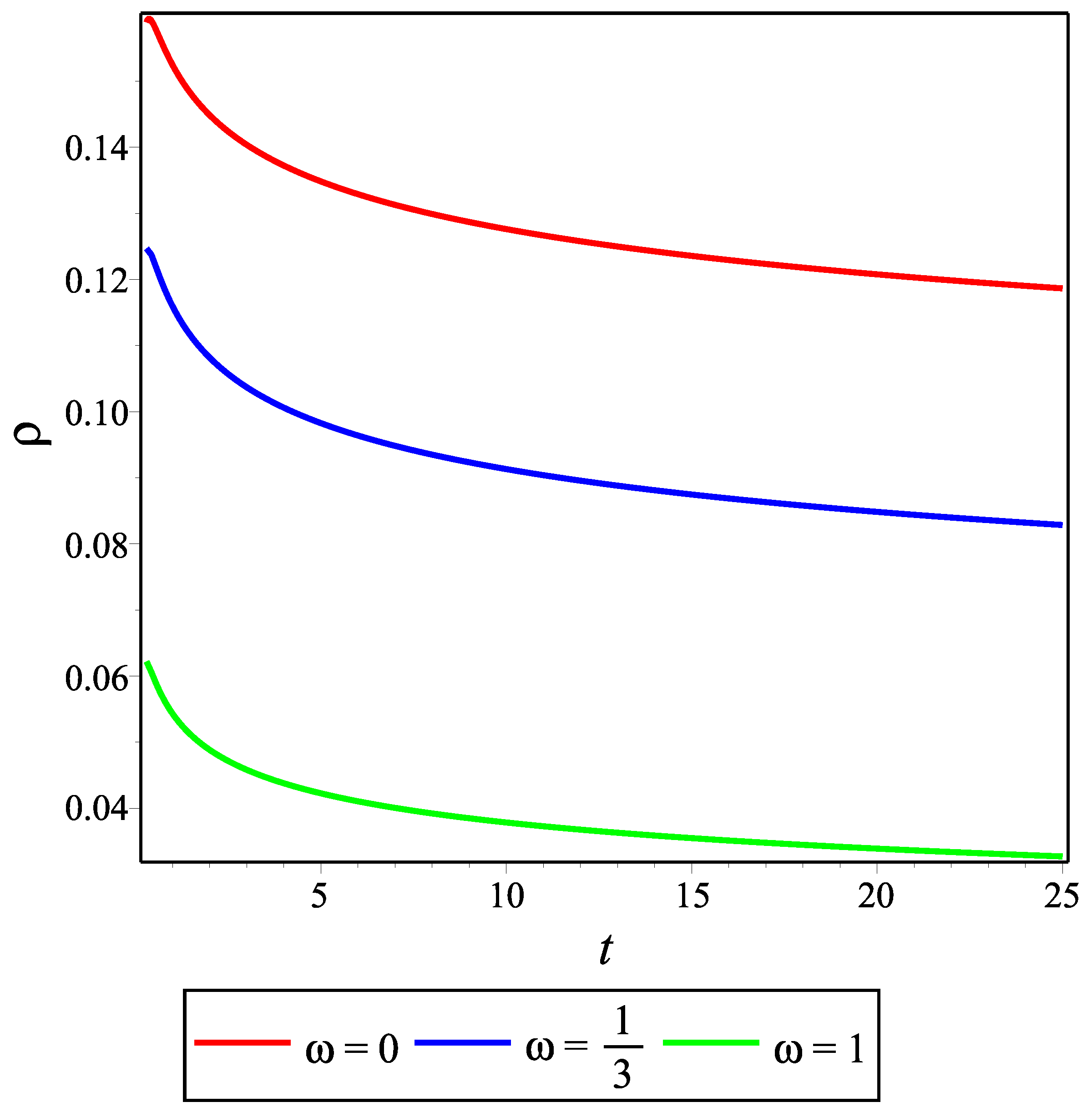
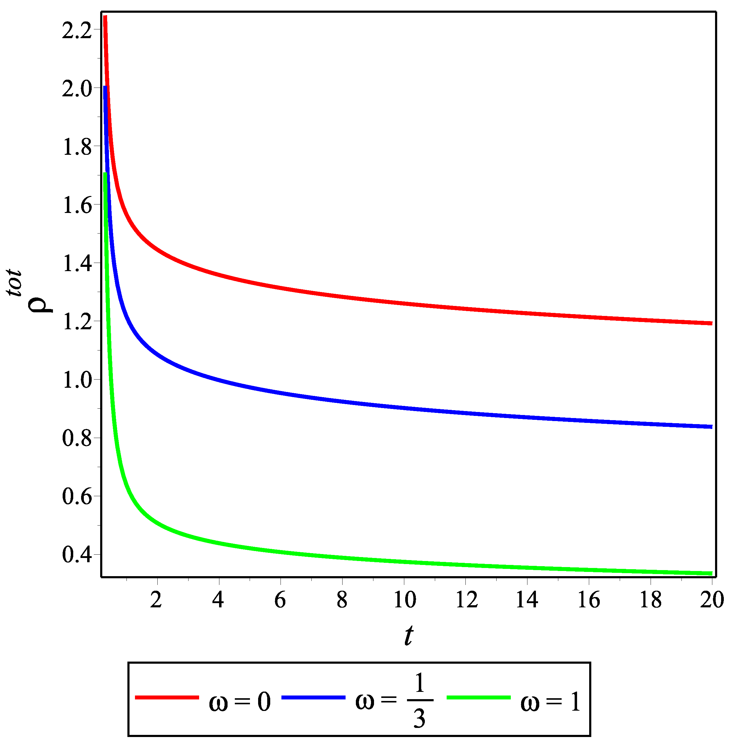
Figure 1, Figure 2 and Figure 3 show the temporal changes in the energy density of matter and the total effective energy density and pressure, respectively, of the decelerating model for the choice of the integration constants , , for the coupling constant and for different positive values of the EoS parameter . We can see from Figure 1 and Figure 2 that and are positive-valued for all t. These are vital conditions for the viability of the model. At the same time, we see from Figure 3 that is always positive, which is consistent with the decelerating universe scenario. In fact, this is the reason for only considering positive values of : the decelerating universe does not contain exotic matter with negative pressure.
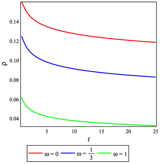
Figure 1.
Evolution of the energy density of matter against time t for decelerating model in NMC form.
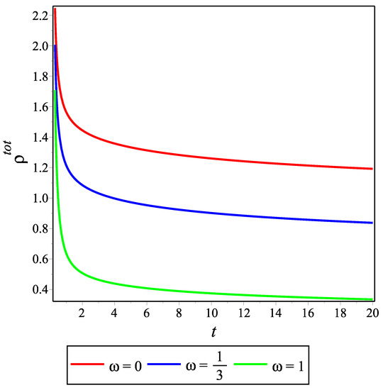
Figure 2.
Evolution of the total effective energy density against time t for decelerating model in NMC form.
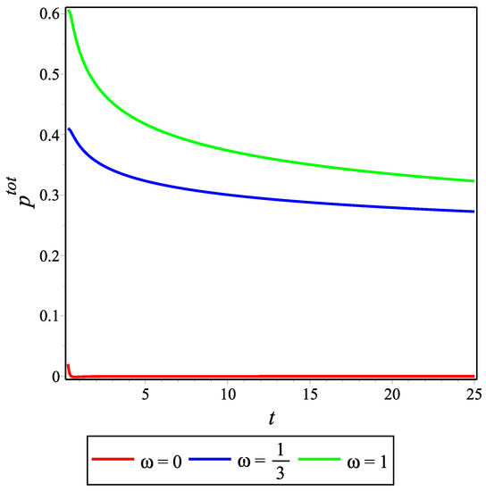
Figure 3.
Evolution of the total effective pressure against time t for decelerating model in NMC form.
4.2. Accelerating Model for NMC Form
The appearance of the negative deceleration parameter indicates that this model is an accelerating model. For this case, if one follows the same procedure as in the previous model, then Equation (26) becomes
and its integration gives
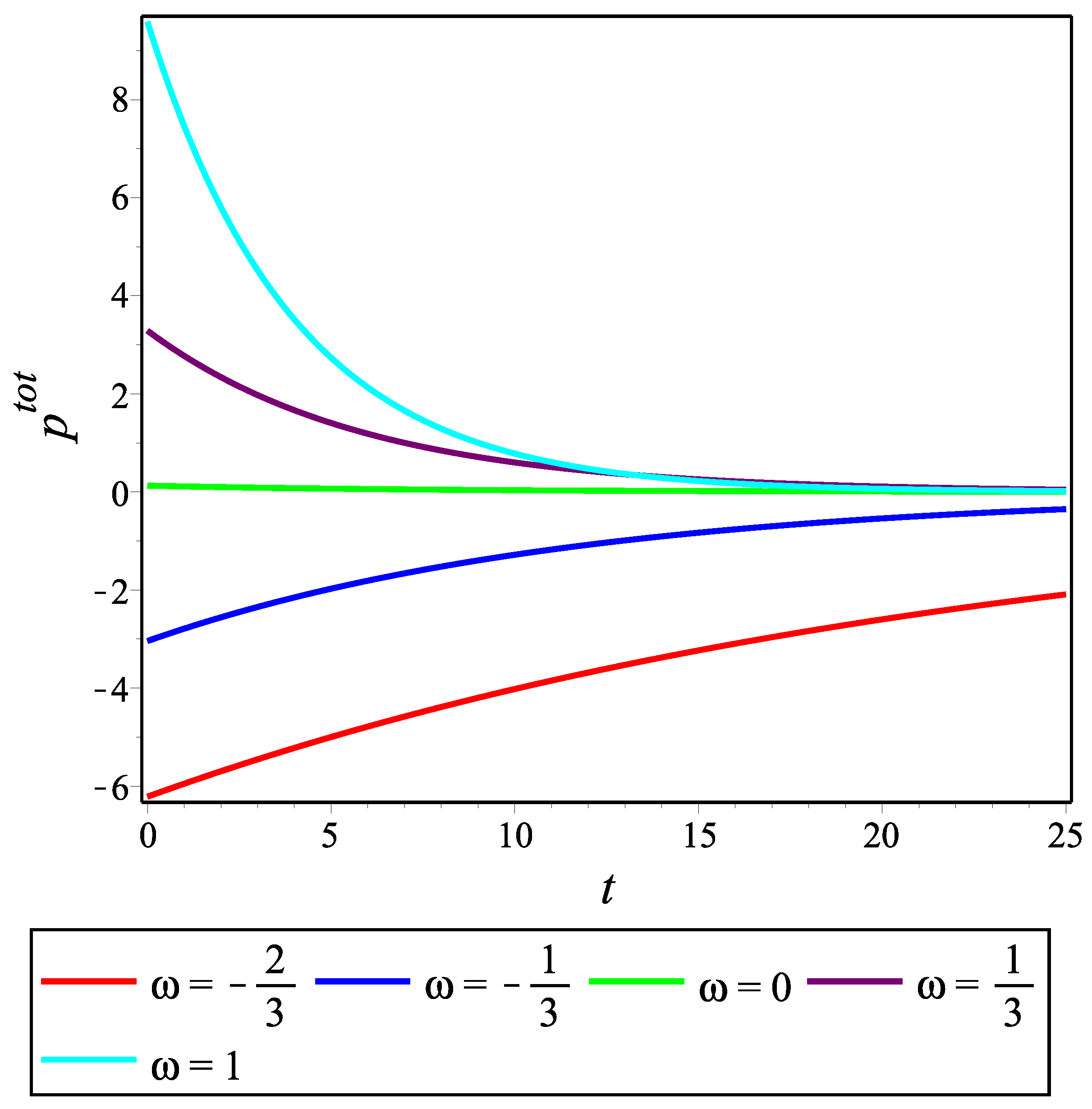
Here again, instead of writing the expressions for and that can be obtained by Equations (28) and (29), we show below how they evolve by using their graphs.
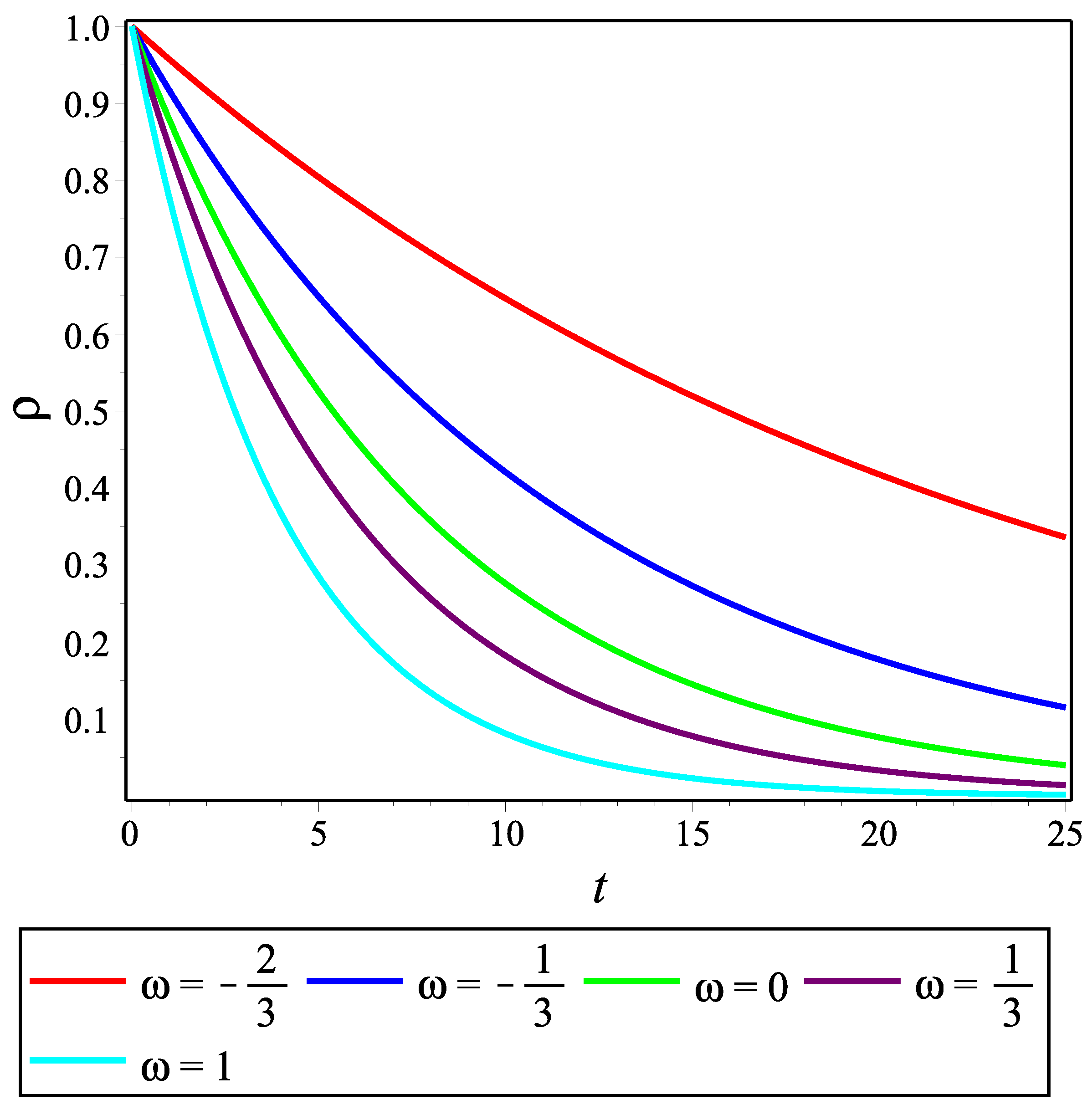
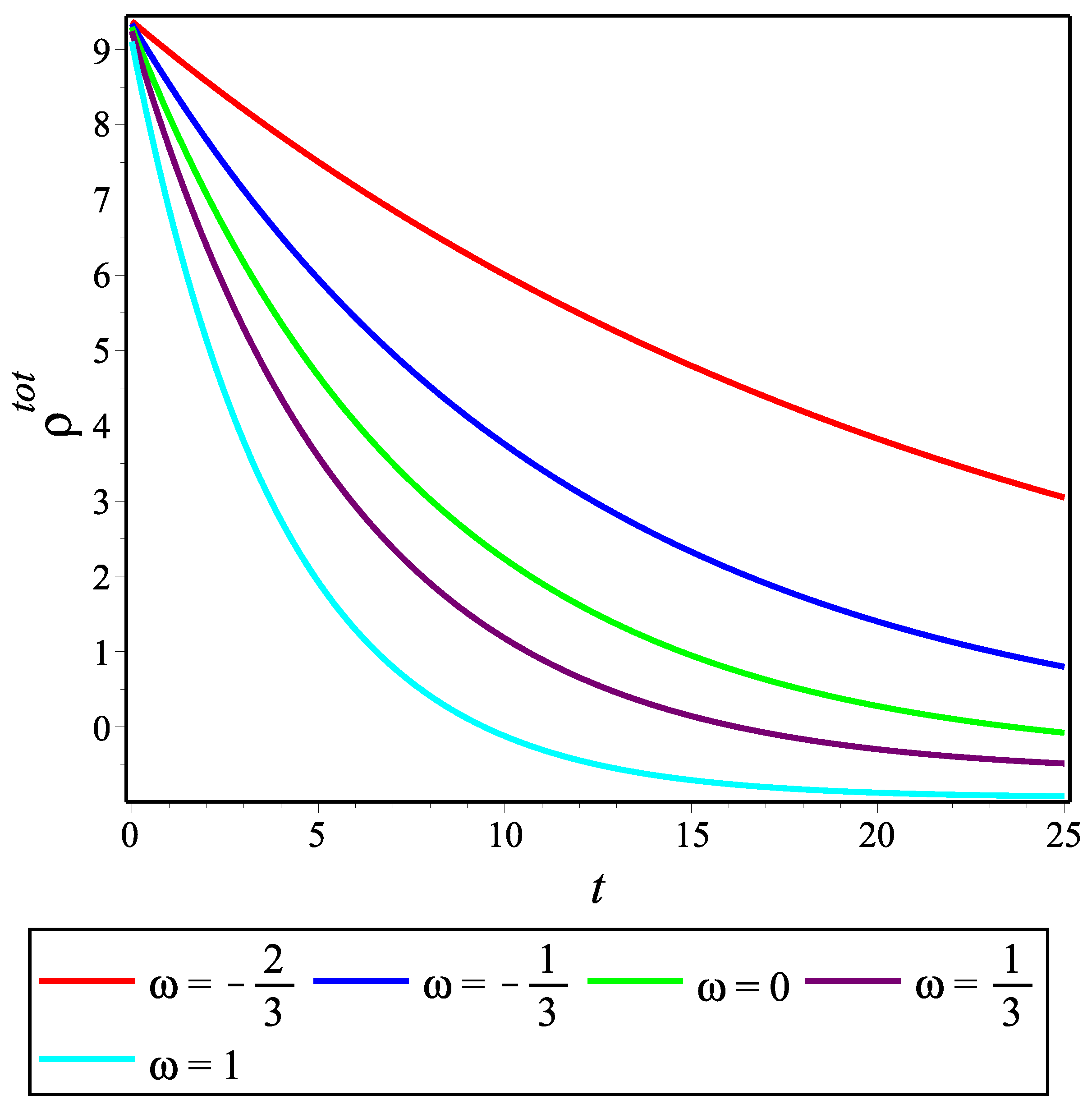
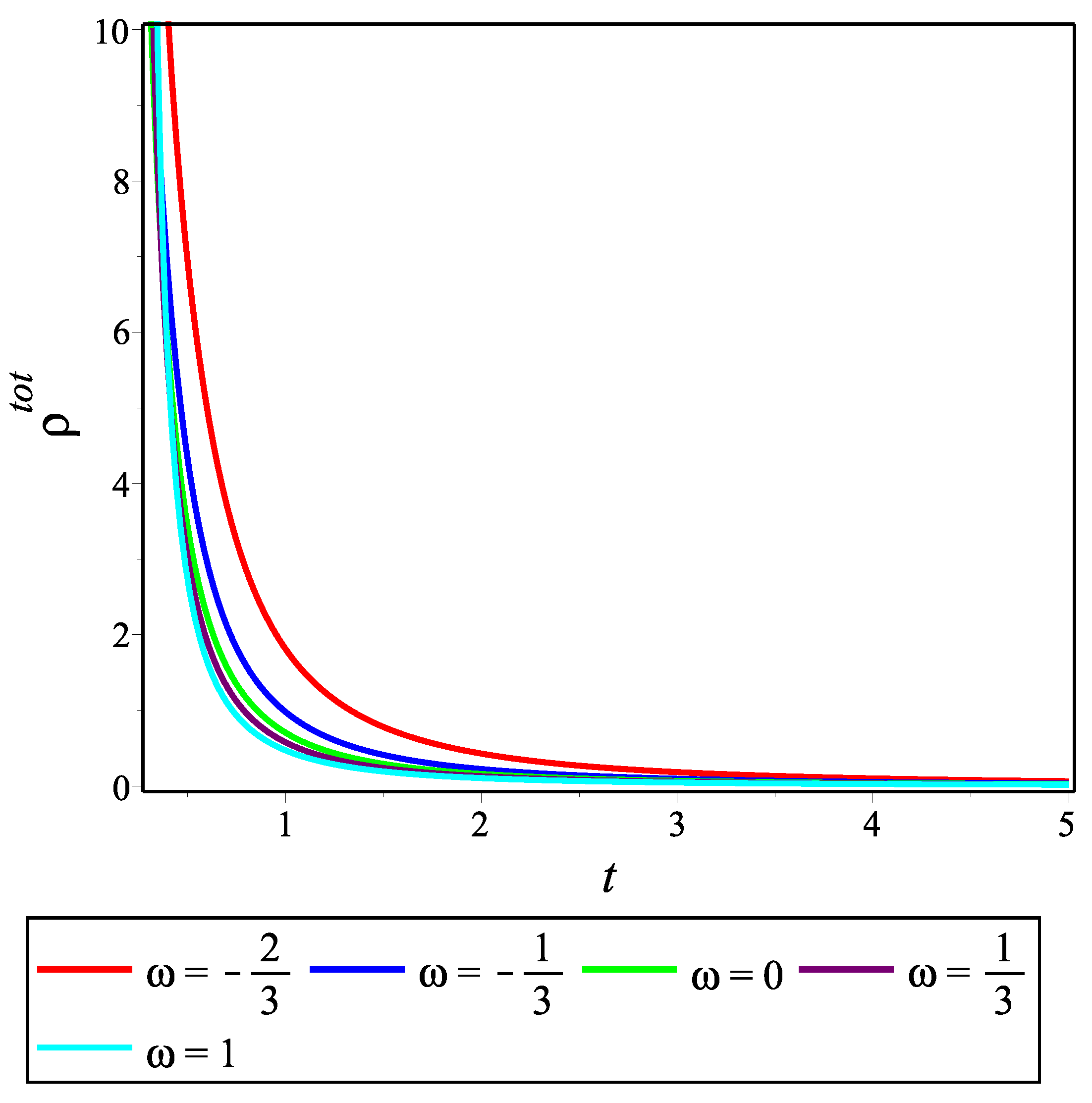
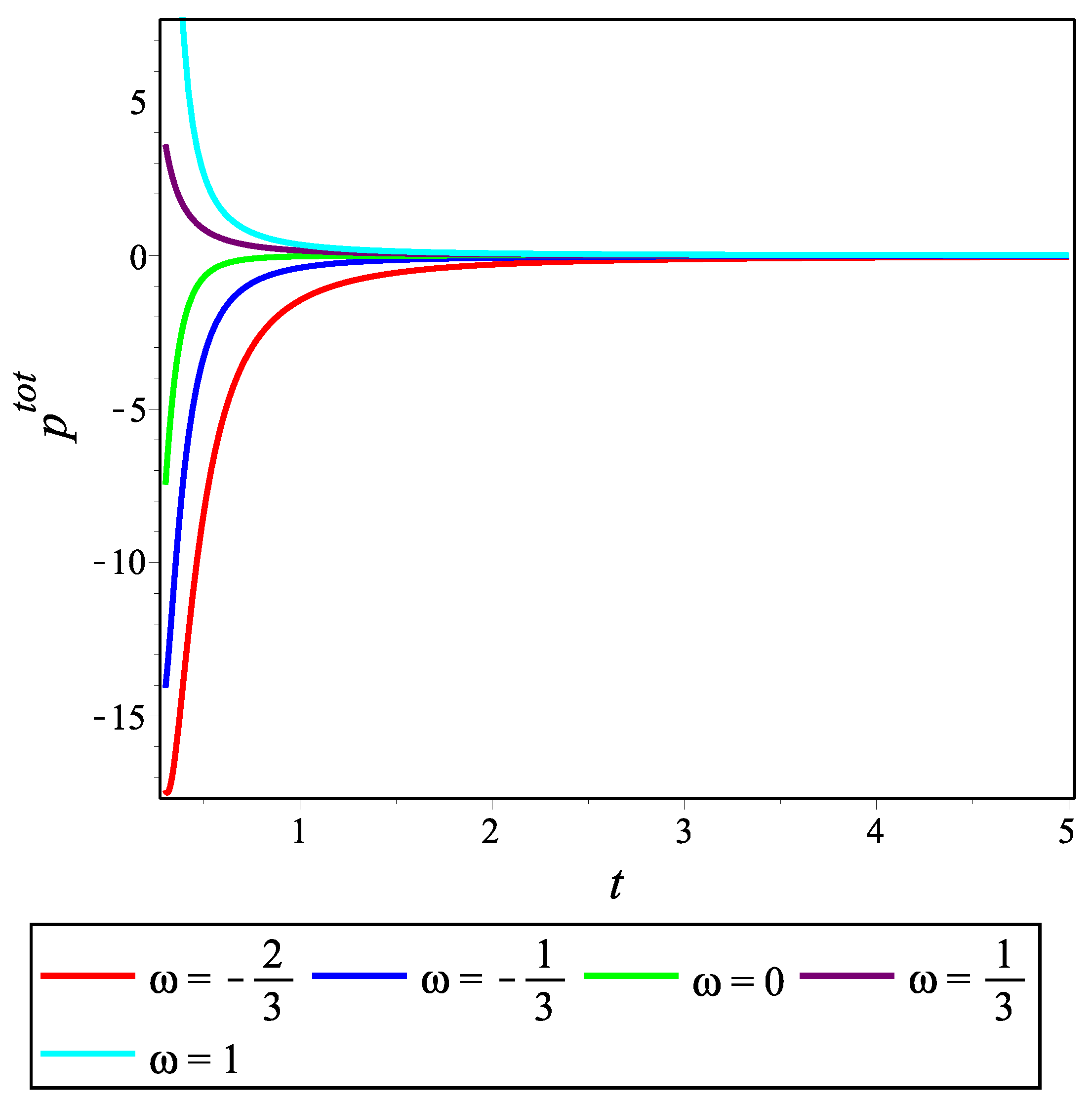
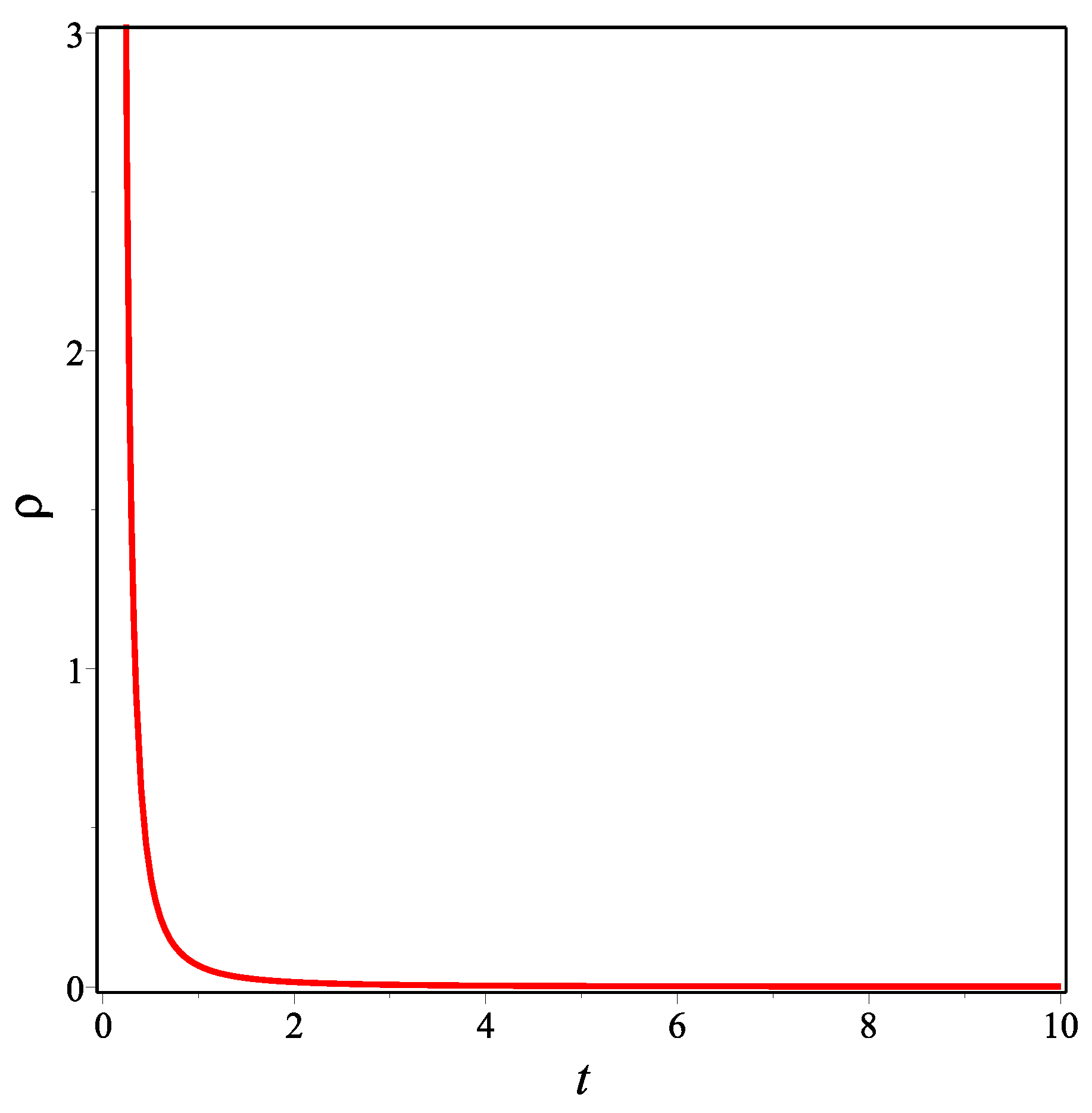
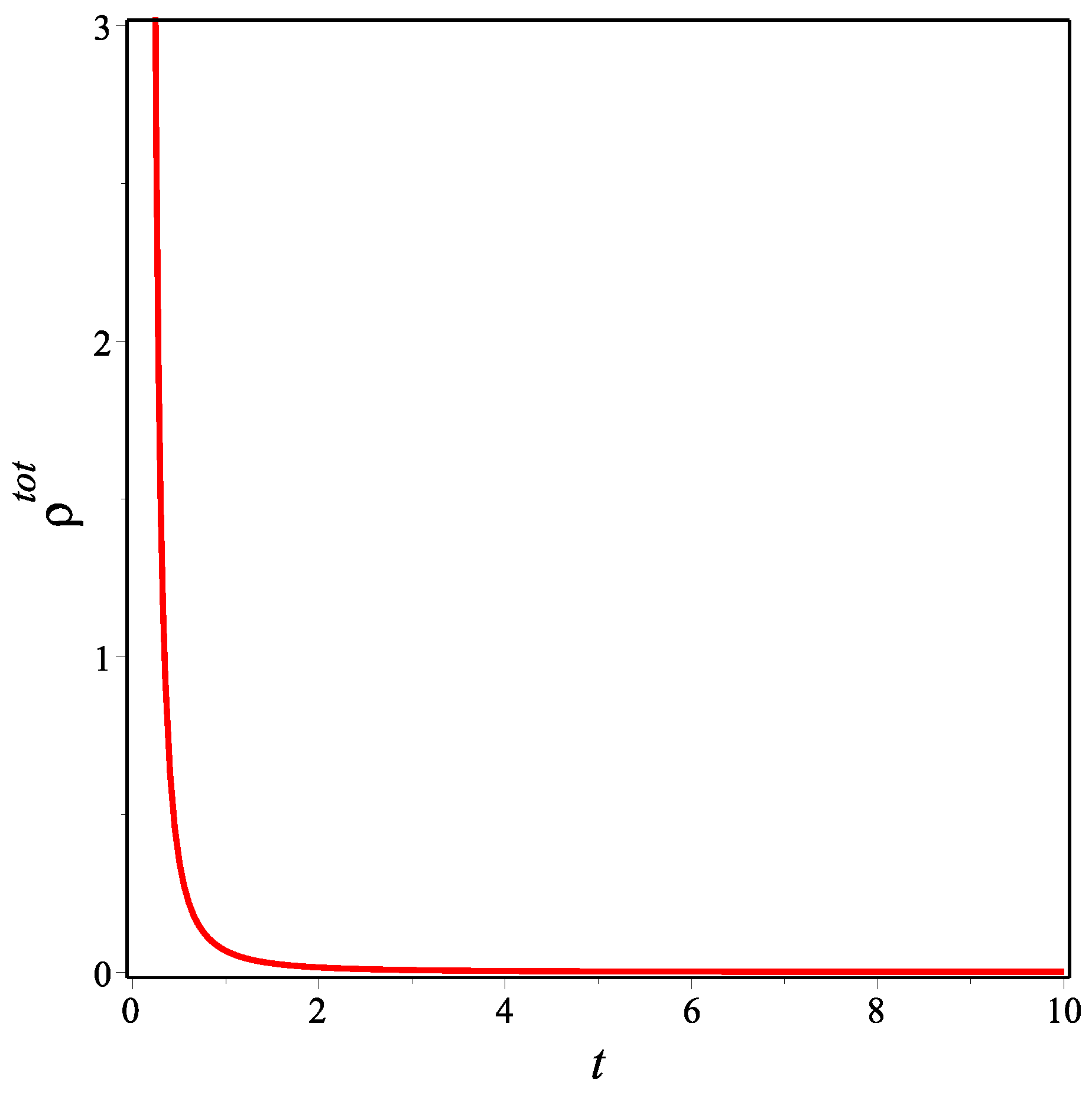
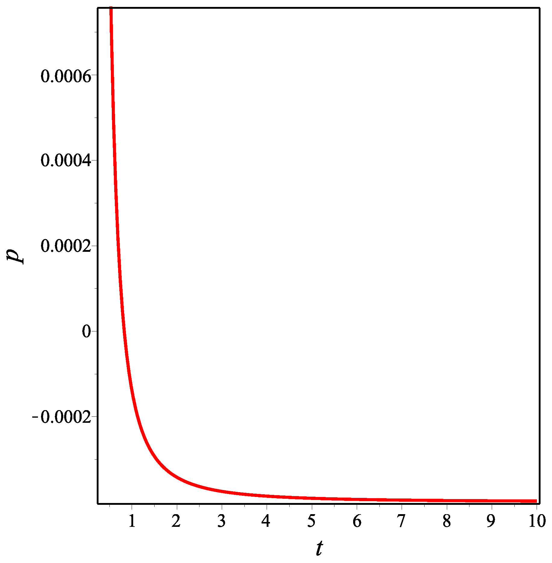
Figure 4, Figure 5 and Figure 6 show the temporal changes in the matter energy density and the total effective energy density and pressure, respectively, of the accelerating model for the choice of constants , , and for different values of the EoS parameter . Unlike the previous model, we take into account both positive and negative values to be compatible with the accelerating universe scenario. We can see that both the densities are positive-valued for all t. Further, can take negative values for negative .

Figure 4.
Evolution of the energy density against time t for accelerating model in NMC form.
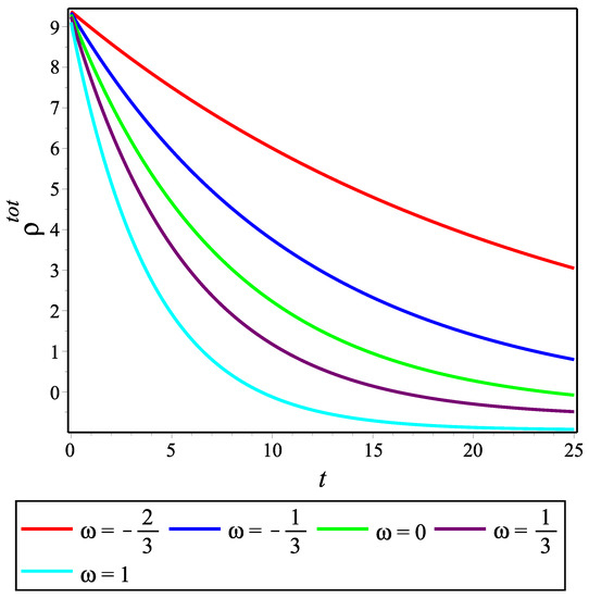
Figure 5.
Evolution of the total effective energy density against time t for accelerating model in NMC form.
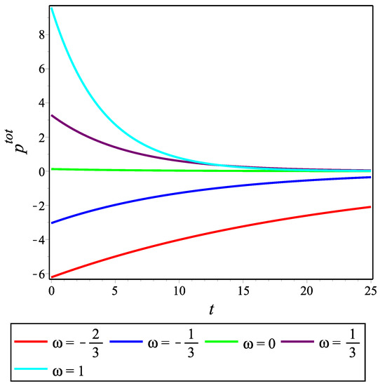
Figure 6.
Evolution of the total effective pressure against time t for accelerating model in NMC form.
4.3. Transit Model for NMC Form
For the transit model incorporating the scale factor a as given by Equation (46), the Hubble and the deceleration parameters are obtained as
Here, we obtain a time-dependent deceleration parameter. A time-dependent deceleration parameter is important for explaining the transition of the expansion of the universe from the past decelerating phase to the recent accelerating phase.
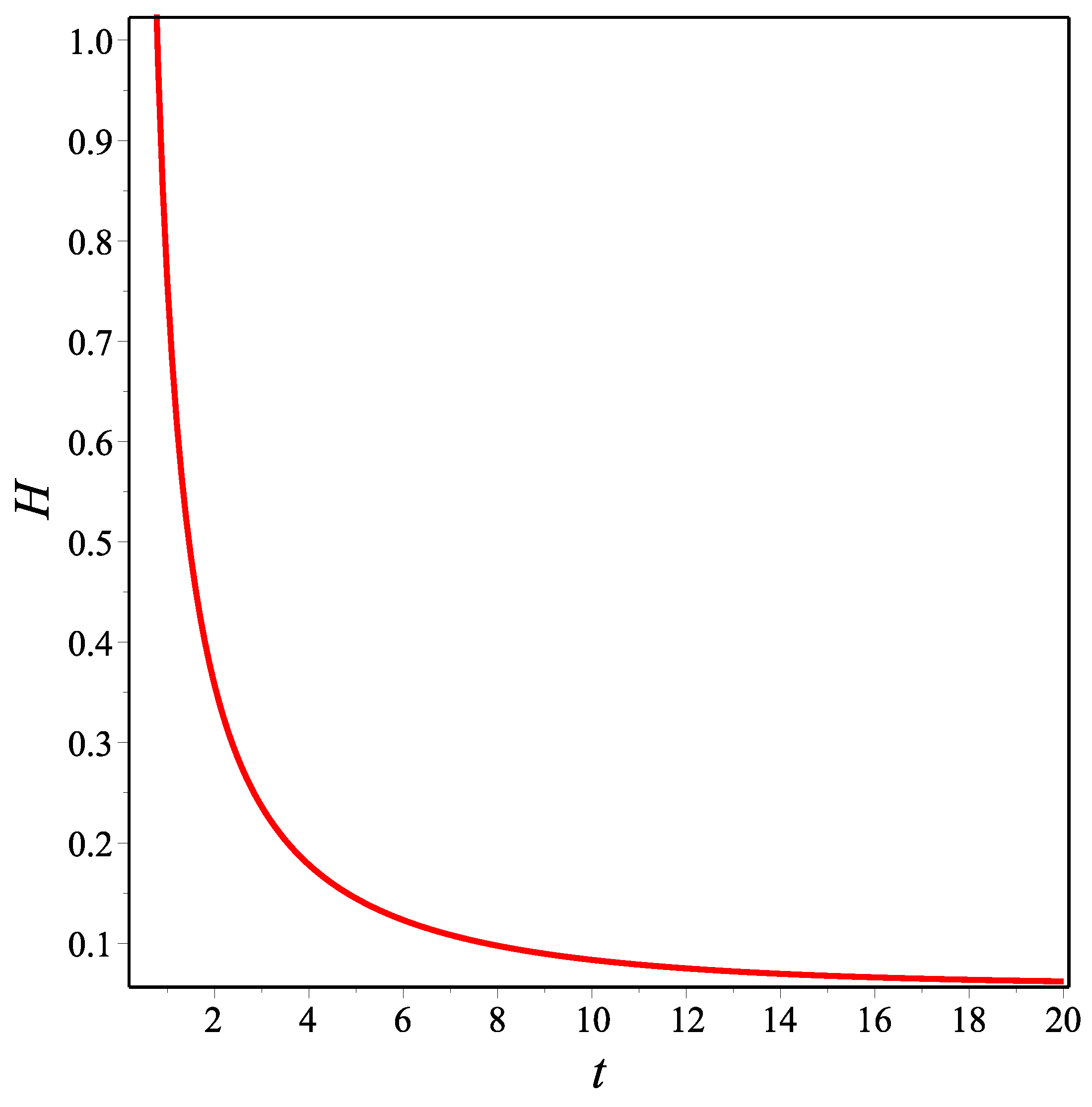
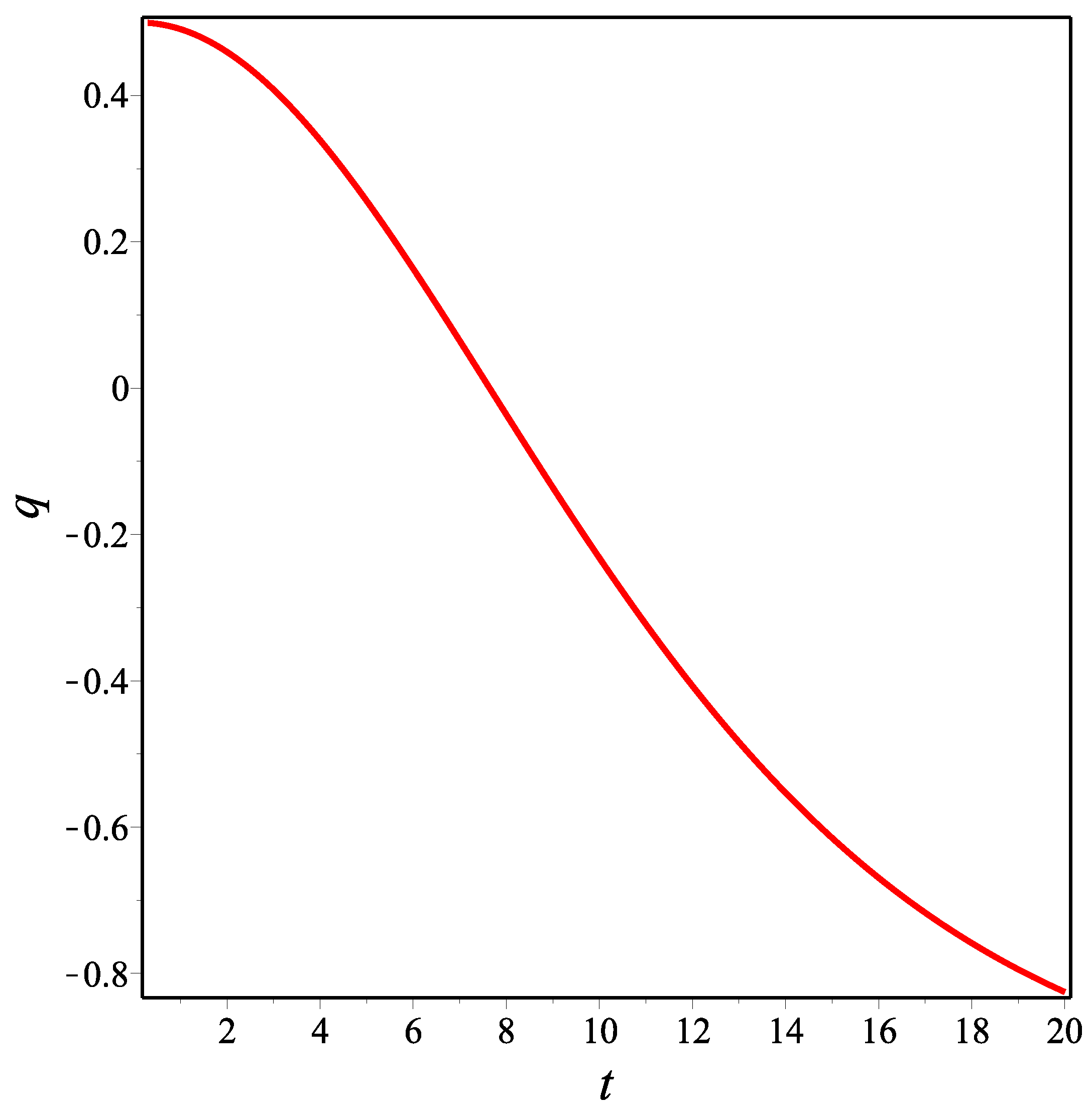
In Figure 7 and Figure 8, the evolutions of the Hubble and deceleration parameters are shown. We see that q exhibits the phase transition from the decelerating to the accelerating expansion phase. In order for the behaviors of q and H and their current values to be compatible with current observations, the values of the constants were chosen as and . According to this, the transition time is almost 7.643 Gyr, the present value of the deceleration paramater is almost , and the present value of the Hubble parameter is almost Gyr. On the other hand, the value of the deceleration parameter at the beginning is , which is the value of q in our decelerating model; and q approaches as t approaches infinity, which is the value of q in our accelerating model.

Figure 7.
Evolution of the Hubble parameter q against time t for transit model.
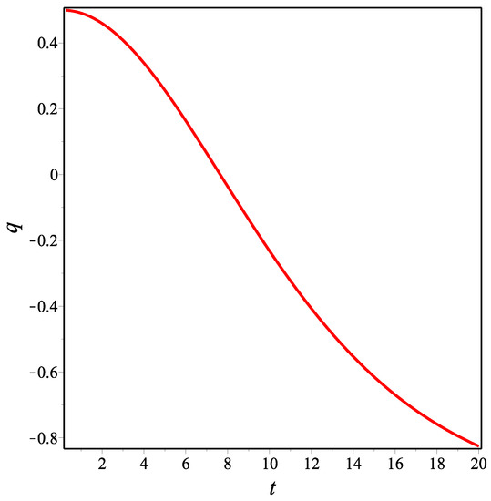
Figure 8.
Evolution of the deceleration parameter q against time t for transit model.
Now, let us discuss the dynamic quantities of this model. In the last two subsections above, we obtained by integrating Equation (26). However, for this model, since an exact solution of the differential Equation (26) cannot be obtained, we obtain using Equation (32). After obtaining , we obtain and by using Equations (23) and (24), respectively. But since all of these expression are quite long, we refrain from writing the expressions of , and here. Instead, we content ourselves with presenting the graphs that show the changes over time, drawn using the values of the constants given above. We can see from Figure 9 and Figure 10 that the energy densities are positive-valued for all values of , while is positive-valued only for positive values of as seen in Figure 11 in this model.
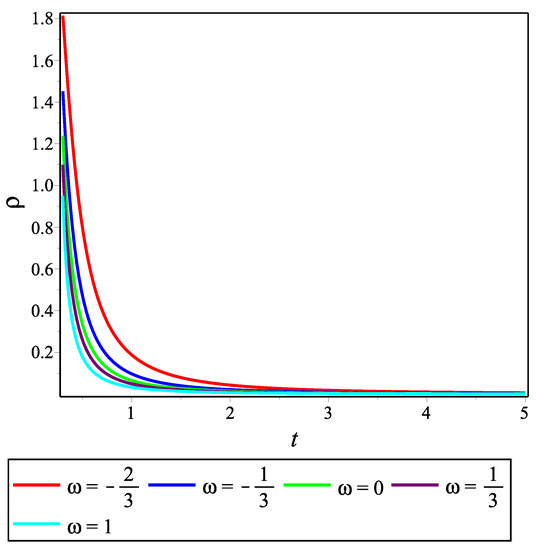
Figure 9.
Evolution of the energy density against time t for transit model in NMC form.
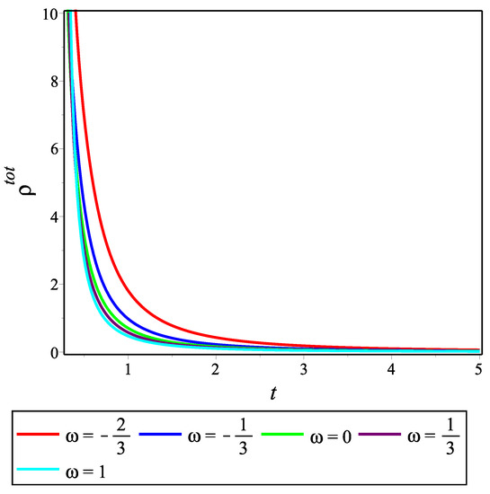
Figure 10.
Evolution of the total effective energy density against time t for transit model in NMC form.
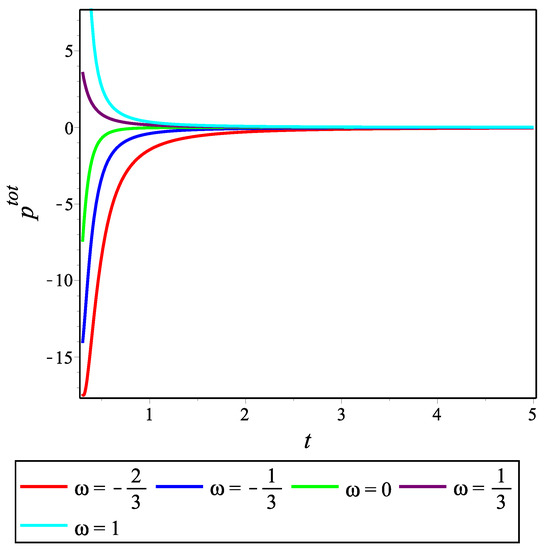
Figure 11.
Evolution of the total effective pressure against time t for transit model in NMC form.
4.4. Decelerating Model for SMC Form
Here, we have obtained the solutions of the energy density and pressure without the need for a constant EoS parameter. However, if we calculate the expression of the EoS parameter using the definition , we still get a constant as follows:
To investigate the time evolution of these dynamical parameters by means of their graphs, an important point to note is that and are connected to each other by Equation (63). Accordingly, the values that we discussed for the decelerating model in the previous subsections are constrained here. The first and obvious restriction is that must be different from 0 because if , then , and this is the GR case. The second constraint, as seen from Equation (63), is that
which tells us that cannot take the value of . The third and final constraint is that ; otherwise, the energy density diverges. Therefore, only the value of remains among the w values we used for the examination of the previous sub-cases. Our examination for this value () gives us the energy density that only takes negative values, ; that is, it has no physical meaning. Consequently, we can interpret that the decelerating expansion solution of the constant jerk parameter is not the solution to the field equations of the SMC form of theory in the flat FLRW background.
4.5. Accelerating Model for SMC Form
For the accelerating model in which , the energy density and pressure given by Equations (37) and (38), respectively, are reduced to constants as follows
Although a positive energy density condition is met for that meets the condition, this situation is not consistent with the expanding universe scenario. Therefore, we can interpret that, as in the previous subsection, the accelerating solution of the constant jerk parameter does not give a physical solution of the field equations of the SMC form.
4.6. Transit Model for SMC Form
For the transit model, in which the scale factor a is given by Equation (46), Equations (37) and (38) become
In this case, the EoS parameter is obtained as
We see that unlike the accelerating model for the SMC form, is not constant in this transit model for the same form.
The behavior of , p and are given in Figure 12, Figure 13, Figure 14 and Figure 15, respectively. As can be seen from these figures, is always positive; p starts its evolution with a positive value, decreases over time, and ends with a negative value; and therefore , while initially taking positive values, decreases over time, goes to zero, and then continues its evolution by taking negative values. It can be seen that converges to as t approaches infinity. In this case, is obtained as a negative constant.
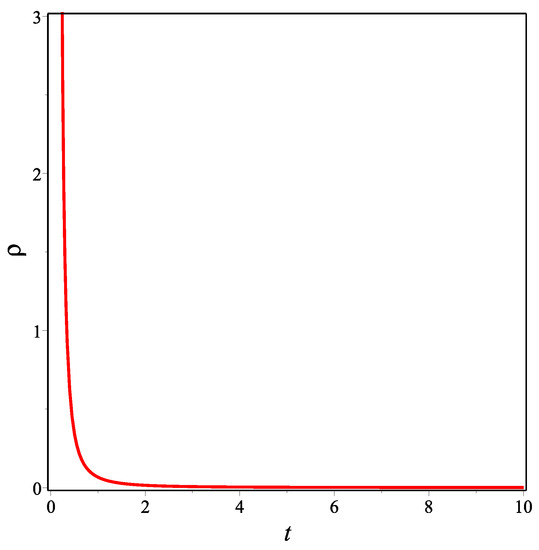
Figure 12.
Evolution of the energy density against time t for transit model in SMC form.
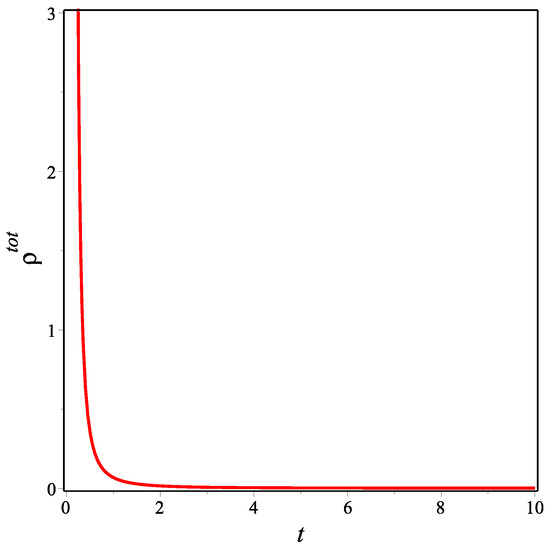
Figure 13.
Evolution of the energy density against time t for transit model in SMC form.
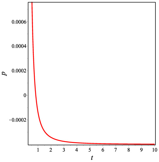
Figure 14.
Evolution of the pressure p against time t for transit model in SMC form.
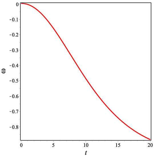
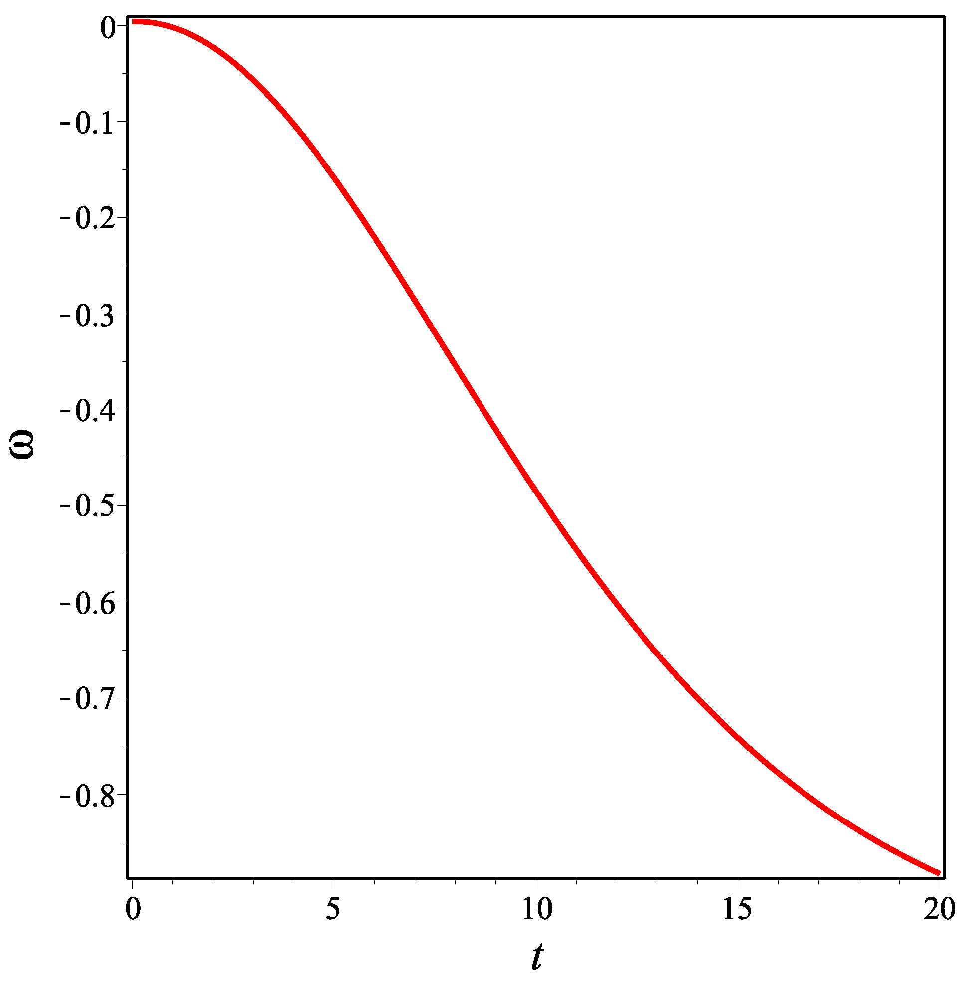
Figure 15.
Evolution of the EoS parameter against time t for transit model in SMC form.
5. Wec Analysis
The condition that the sum of the energy density and pressure is not negative must also be satisfied, as well as the requirement for a positive energy density for any physically valid cosmological model. The requirement of these two conditions together is called the weak energy condition (WEC). In addition, in modified gravity theories, the WEC is generalized and similar conditions must be satisfied for the effective fluid. The generalized WEC demands
and
Since the SMC form of the models we discussed above does not give the desired solutions for both the accelerating and decelerating models, we now analyze the WEC only for the NMC form. Therefore, from now on, we use the decelerating and accelerating model expressions (unless otherwise specified) only for the NMC form. But for the transition model, we consider both the NMC and SMC forms in the following.
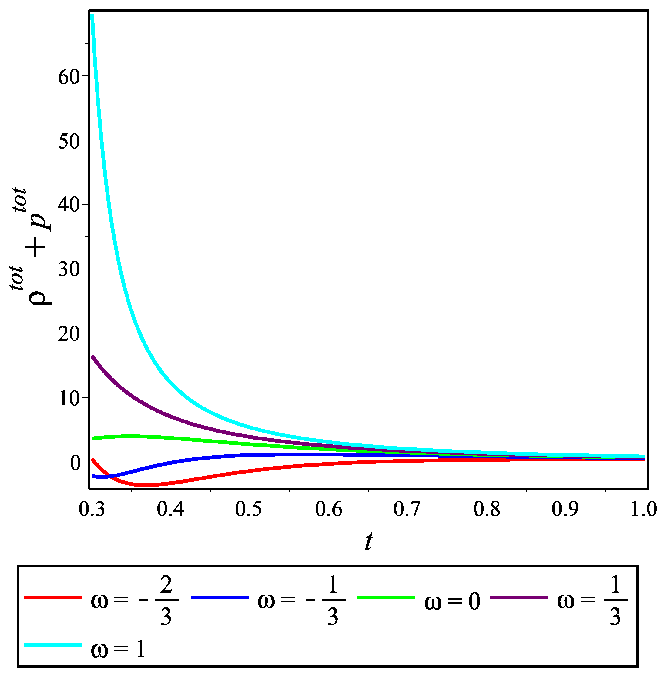
The conditions (71) are satisfied for all the decelerating, accelerating and transit models we have discussed above and are illustrated in Figure 1, Figure 2, Figure 4, Figure 5, Figure 9, Figure 10, Figure 12 and Figure 13. Now, the conditions (72) are illustrated again in Figure 16, Figure 17, Figure 18, Figure 19, Figure 20, Figure 21, Figure 22 and Figure 23.
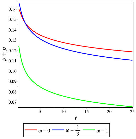
Figure 16.
Evolution of against time t for decelerating model in NMC form.

Figure 17.
Evolution of against time t for decelerating model in NMC form.
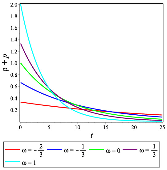
Figure 18.
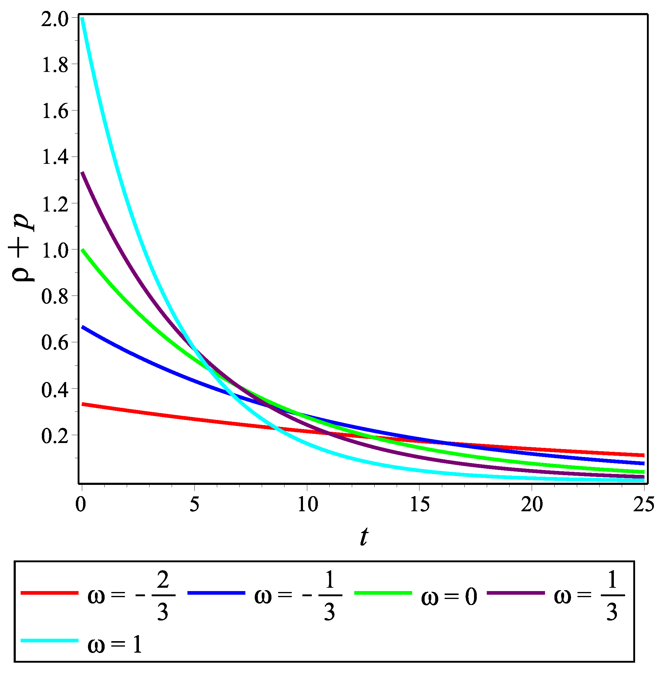
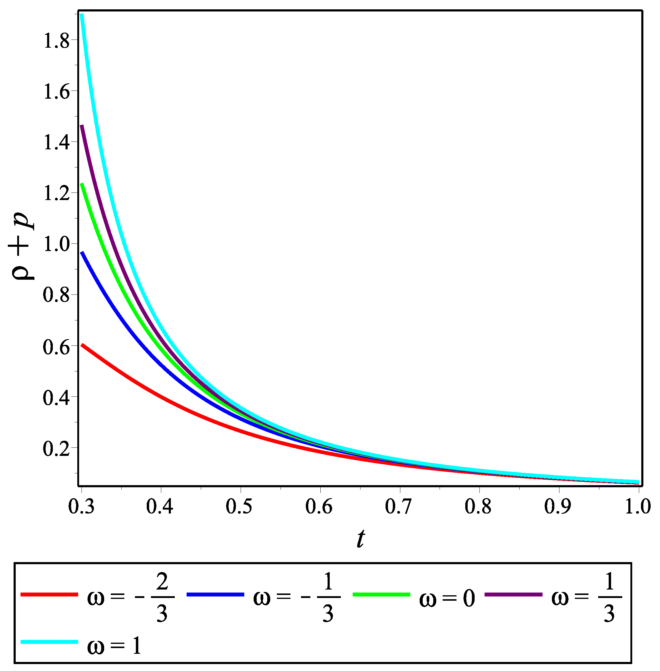
Evolution of against time t for accelerating model in NMC form.
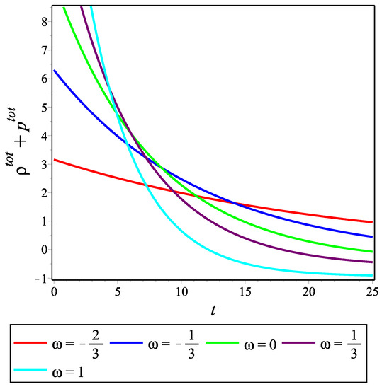
Figure 19.
Evolutionof against time t for accelerating model in NMC form.
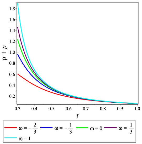
Figure 20.
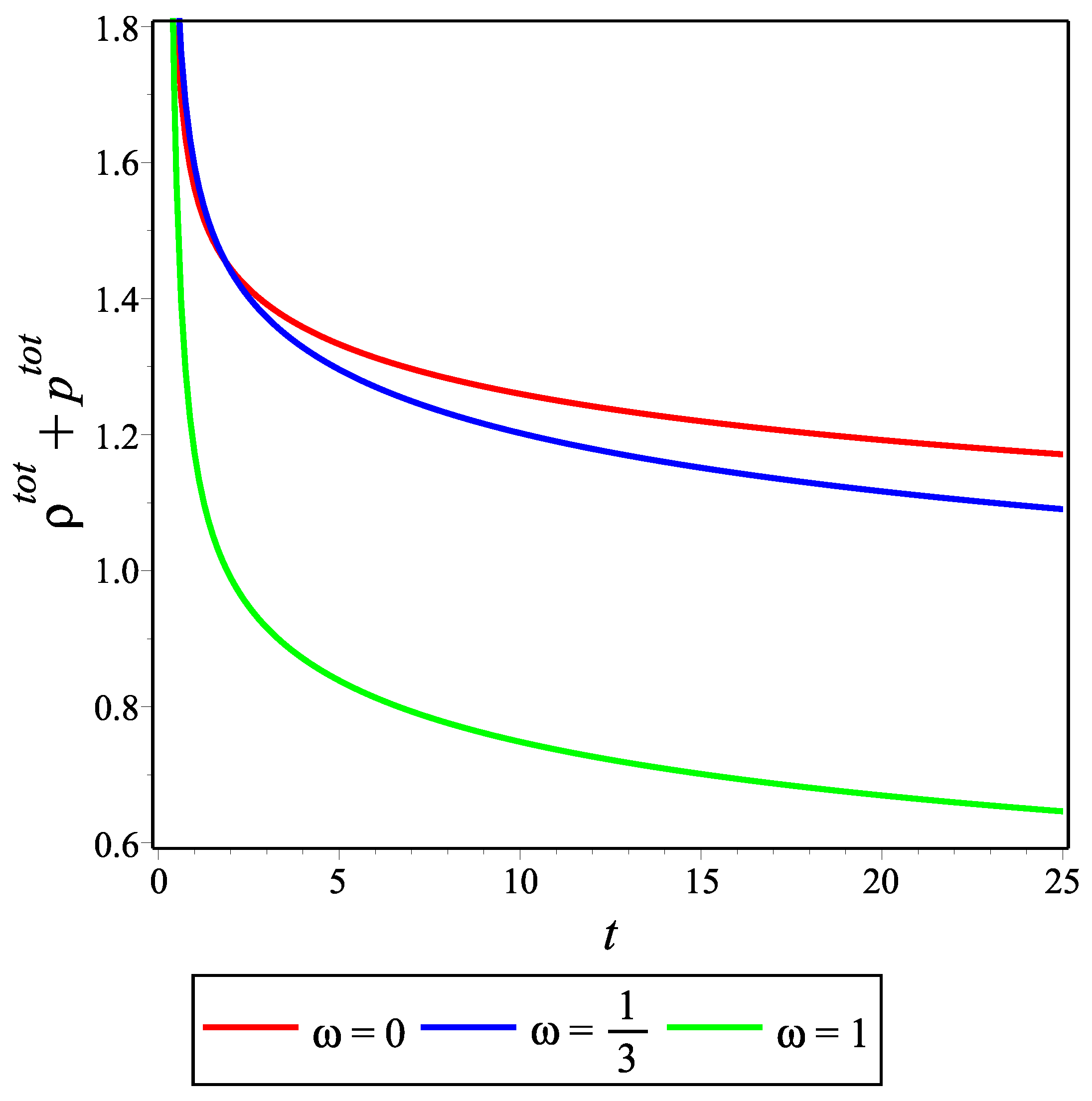
Evolutionof against time t for transit model in NMC form.
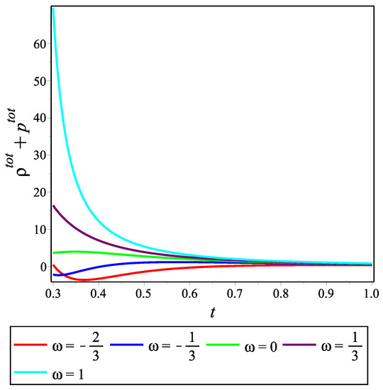
Figure 21.
Evolution of against time t for transit model in NMC form.
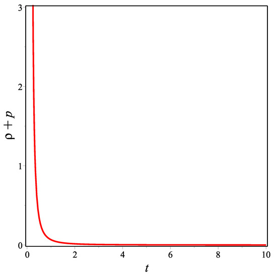
Figure 22.
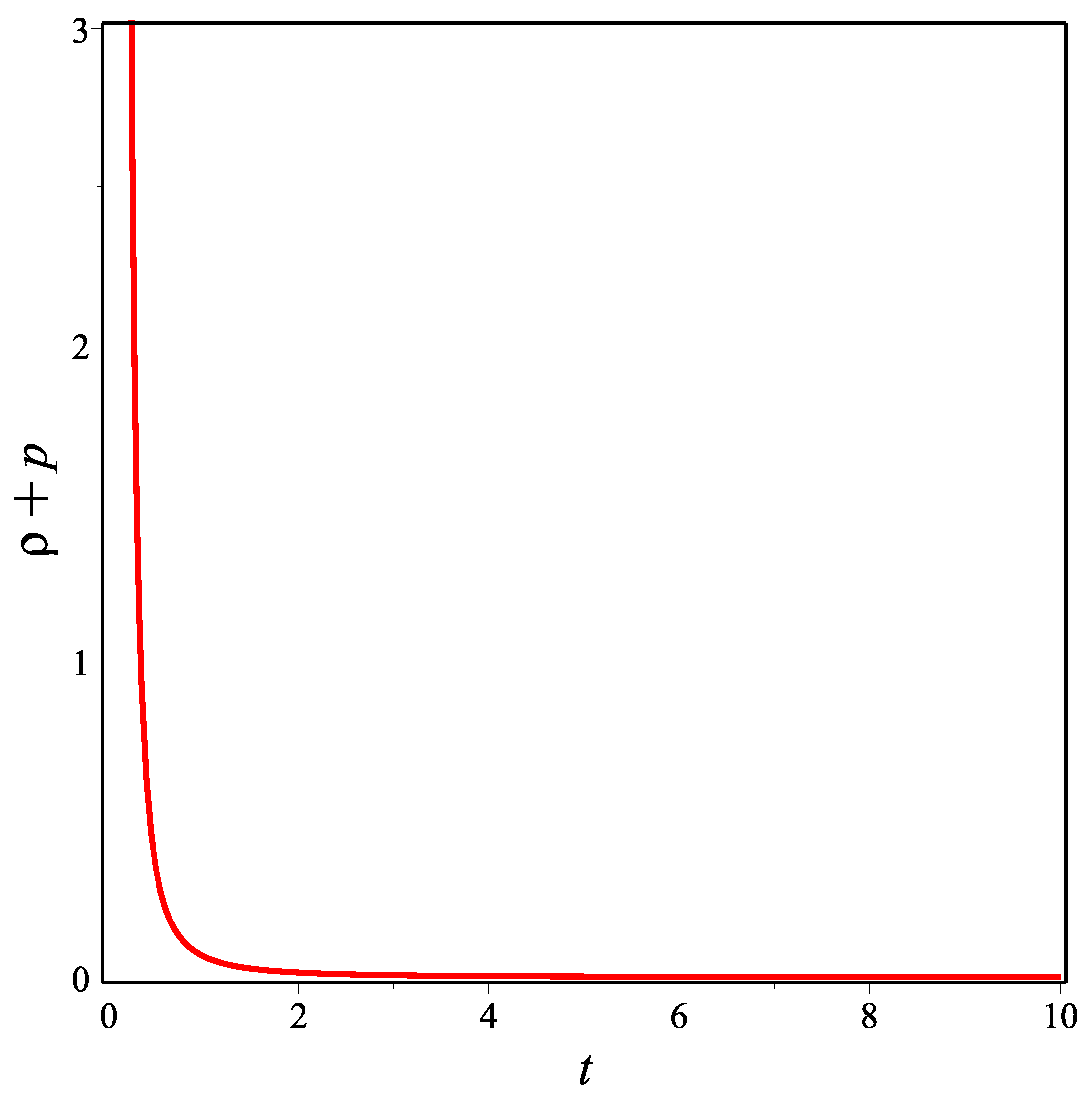
Evolution of against time t for transit model in SMC form.
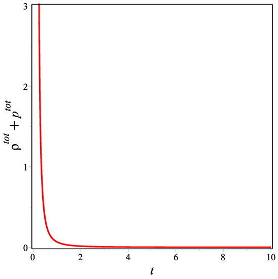
Figure 23.
Evolution of against time t for transit model in SMC form.
We can see from Figure 16 and Figure 17 that conditions (72) are satisfied in the decelerating model for all selected values of . On the other hand, while the first condition of (72) is satisfied in the accelerating model, as seen from Figure 18, its second condition is satisfied only for negative values of . In the transit model for the NMC form, the first condition is satisfied for all selected values of , while the second condition is not satisfied for negative values of . Also, the condition is satisfied, as seen in Figure 23, in the transit model for the SMC form. Thus, there are different situations for which the WEC is satisfied for the decelerating and accelerating models in the NMC form and for the transit models in both the NMC and SMC forms that we consider in this study.
6. Conclusions
We have studied dark energy with a constant jerk parameter in an FLRW model in gravity. The simplest form , is usually studied in the literature. For this reason, to compare our results, we also discussed the simplest case as well as the more complicated form. In the papers [20,21], the authors also studied a constant jerk parameter in a Bianchi I model in gravity, but they used the form , , so that work is different from ours.
This theory does not have energy conservation, but energy can be lost or gained or particle production may occur. This is similar to having a more generalized energy–momentum tensor, including viscosity or heat conduction in GR.
In the standard CDM model in GR, which fits observational constraints reasonably well, we have . We expect any generalized cosmological model to tend to the CDM model at late times. By choosing as a starting point, we obtained, for the first time we believe, Equations (40)–(45). However, since these solutions are complicated, we chose one of them, viz., (41), and were able to write it as Equation (46). We call this solution the transit solution. However, a power law solution Equation (47) and an exponential solution Equation (48) are also exact solutions to the differential equation for . The power law solution is valid at early times, and the exponential solution applies at late times. We analyzed these three solutions separately. Hence, by choosing as a starting point, we ensured that the relevant model approximates that of the CDM model at late times. We have plotted the energy densities, effective energy densities and effective pressures for the decelerating model in Figure 1, Figure 2 and Figure 3, for the accelerating model in Figure 4, Figure 5 and Figure 6 and for the transit model in NMC form in Figure 9, Figure 10 and Figure 11.
A detailed energy analysis of the weak energy condition has been carried out, and the decelerating model satisfies the WEC. The accelerating model satisfies the WEC except for positive values of . Conversely, the transit model satisfies the WEC except for negative values of . These results are illustrated in Figure 16, Figure 17, Figure 18, Figure 19, Figure 20, Figure 21, Figure 22 and Figure 23. We have also plotted the Hubble and deceleration parameters for the transit model in Figure 7 and Figure 8, showing that the transition time is Gyr and that the present values of the Hubble and deceleration parameters are consistent with recent observational values.
Finally, we mentioned in the introduction that this work is based on an earlier abbreviated paper [19] that appeared in the Proceedings of the 2nd Electronic Online Conference on the Universe held during 16 February–2 March 2023. We shall now point out briefly what was done in that paper along with the novel aspects in this work. In our earlier paper, we chose a nonlinear functional form for , given by . For the flat FLRW metric, we worked out the field equations and then chose the jerk parameter to be . Since this nonlinear differential equation was difficult to solve, we managed to only find exact power law and exponential solutions at that stage. The former represents deceleration, and the latter represents acceleration. We also found the expressions for the energy density for both solutions, and we plotted these.
In this work, the novel aspects are:
- This study entails a much deeper analysis of the concept of the implications of a constant jerk parameter for modified gravity.
- Most studies of theory are based on the linear form of . In this work, we considered the nonlinear form . This is much more difficult to analyze.
- The complete solution to the differential Equation (39) for has been presented for the first time here as far as we are aware.
- Since these equations are fairly complicated, and some of them are complex (and therefore imaginary), we selected one of the solutions. We simplified it to a manageable form that could be analyzed more easily, and we provided a complete analysis of this solution (the transit solution).
- Using observations, we calculated the values of the parameters that occur in the transit solution. Then, we calculated the Hubble parameter at the present time, the deceleration parameter at present and at transition, and the transition time from deceleration to acceleration. The transit solution appears to be viable, but we plan a more detailed analysis of its implications in the future, including observations.
- The transit solution was compared with the two other solutions (power law and exponential). Detailed plots were provided for all three solutions to illustrate the results more clearly.
- Energy conditions were analyzed in this paper; these were not addressed in the Phys. Sc. Forum paper. These conditions were analyzed in detail for all three types of models, and detailed comparisons were made amongst all three.
- This work has 23 figures illustrating our results here, as compared to 2 in the previous work.
Author Contributions
Conceptualization, D.S. and A.B.; methodology, D.S.; software, D.S.; validation, D.S. and A.B.; formal analysis, D.S. and A.B.; investigation, D.S. and A.B.; resources, D.S.; writing—original draft preparation, D.S.; writing—review and editing, D.S. and A.B.; supervision, D.S. and A.B.; project administration, D.S. and A.B. All authors have read and agreed to the published version of the manuscript.
Funding
This research received no external funding.
Institutional Review Board Statement
Not applicable.
Informed Consent Statement
Not applicable.
Data Availability Statement
No new data were created or analyzed in this study. Data sharing is not applicable to this article.
Acknowledgments
The authors would sincerely like to thank all the reviewers for their enlightening comments, which have helped improve the manuscript considerably.
Conflicts of Interest
The authors declare no conflict of interest.
Abbreviations
The following abbreviations are used in this manuscript:
| GR | General Relativity |
| DE | Dark Energy |
| CDM | Cold Dark Matter |
| WEC | Weak Energy Condition |
References
- Permutter, S.; Aldering, G.; Goldhaber, G.; Knop, R.A.; Nugent, P.G.; Castro, P.G.; Deustua, S.; Fabbro, S.; Goobar, A.; Groom, D.E.; et al. Observational Evidence from Supernovae for an Accelerating Universe and a Cosmological Constant. Astrophys. J. 1999, 517, 565–586. [Google Scholar]
- Riess, A.G.; Filippenko, A.V.; Challis, P.; Clocchiatti, A.; Diercks, A.; Garnavich, P.M.; Gilliland, R.L.; Hogan, C.J.; Jha, S.; Kirshner, R.P.; et al. Observational Evidence from Supernovae for an Accelerating Universe and a Cosmological Constant. Astron. J. 1998, 116, 1009–1038. [Google Scholar] [CrossRef]
- Riess, A.G.; Kirshner, R.P.; Schmidt, B.P.; Jha, S.; Challis, P.; Garnavich, P.M.; Esin, A.A.; Carpenter, C.; Grashius, R. The American Astronomical Society, find out more The Institute of Physics, find out more BVRI Light Curves for 22 Type Ia Supernovae. Astron. J. 1999, 117, 707–724. [Google Scholar] [CrossRef]
- Ade, P.A.R.; Aghanim, N.; Arnaud, M.; Ashdown, M.; Aumont, J.; Baccigalupi, C.; Banday, A.J.; Barreiro, R.B.; Bartlett, J.G.; Bartolo, N.; et al. Planck 2015 results. XIII. Cosmological parameters. Astron. Astrophys. 2016, 594, A13. [Google Scholar]
- Ratra, B.; Peebles, P.J.E. Cosmological consequences of a rolling homogeneous scalar field. Phys. Rev. D 1988, 37, 3406. [Google Scholar] [CrossRef]
- Wetterich, C. Cosmology and the fate of dilatation symmetry. Nucl. Phys. B 1988, 302, 668–696. [Google Scholar] [CrossRef]
- Khurshudyan, M.; Chubaryan, E.E.; Pourhassan, B. Inteeracting quintessence models of dark energy. Int. J. Theor. Phys. 2014, 53, 2370–2378. [Google Scholar] [CrossRef]
- Armendariz-Picon, C.; Mukhanov, V.; Steinhardt, P.J. Dynamical Solution to the Problem of a Small Cosmological Constant and Late-Time Cosmic Acceleration. Phys. Rev. Lett. 2000, 85, 4438. [Google Scholar] [CrossRef]
- Kamenshchik, A.Y.; Moschella, U.; Pasquier, V. An alternative to quintessence. Phys. Lett. B 2001, 511, 265–268. [Google Scholar] [CrossRef]
- Bento, M.C.; Bertolami, O.; Sen, A.A. Generalized Chaplygin gas, accelerated expansion, and dark-energy-matter unification. Phys. Rev. D 2002, 66, 043507. [Google Scholar] [CrossRef]
- Xu, L.; Lu, J.; Wang, Y. Revisiting generalized Chaplygin gas as a unified dark matter and dark energy model. Eur. Phys. J. C 2012, 72, 1883. [Google Scholar] [CrossRef]
- Saadat, H.H.; Pourhassan, B. FRW Bulk Viscous Cosmology with Modified Chaplygin Gas in Flat Space. Astrophys. Space Sci. 2013, 344, 237. [Google Scholar] [CrossRef]
- Pourhassan, B. Viscous modified cosmic Chaplygin gas cosmology. Int. J. Mod. Phys. D 2013, 22, 1350061. [Google Scholar] [CrossRef]
- Harko, T.; Lobo, F.S.N.; Nojiri, S.; Odintsov, S.D. f(R,T) gravity. Phys. Rev. D 2011, 84, 024020. [Google Scholar] [CrossRef]
- Moraes, P.H.R.S.; Sahoo, P.K. The simplest non-minimal matter-geometry coupling in the f(R,T) cosmology. Eur. Phys. J. C 2017, 77, 480. [Google Scholar] [CrossRef]
- Sharma, L.K.; Yadav, A.K.; Sahoo, P.K.; Singh, B.K. Non-minimal matter-geometry coupling in Bianchi I space-time. Results Phys. 2018, 10, 738–742. [Google Scholar] [CrossRef]
- Tiwari, R.K.; Sofuoglu, D.; Isik, R.; Shukla, B.K.; Baysazan, E. Non-minimally coupled transit cosmology in f(R,T) gravity. Int. J. Geom. Meth. Mod. Phys. 2022, 19, 2250118. [Google Scholar] [CrossRef]
- Sofuoglu, D.; Tiwari, R.K.; Abebe, A.; Alfedeel, A.H.A.; Hassan, E.I. The cosmology of a non-minimally coupled f(R,T) gravitation. Physics 2022, 4, 1348–1358. [Google Scholar] [CrossRef]
- Sofuoglu, D.; Beesham, A. f(R, T) Gravity and Constant Jerk Parameter in FLRW Spacetime. Phys. Sci. Forum 2023, 7, 13. [Google Scholar]
- Tiwari, R.K.; Sofuoglu, D.; Mishra, S.K. and Beesham, A. Anisotropic model with constant jerk parameter in f(R,T) gravity. Gravit. Cosmol. 2022, 28, 196–203. [Google Scholar] [CrossRef]
- Tiwari, R.K.; Kumar, S.; Dubey, V.K.; Sofuoglu, D. Role of constant jerk parameter in f(R, T) gravity. Int. J. Geom. M. Mod. Phys. 2023, 20, 2350049. [Google Scholar] [CrossRef]


Disclaimer/Publisher’s Note: The statements, opinions and data contained in all publications are solely those of the individual author(s) and contributor(s) and not of MDPI and/or the editor(s). MDPI and/or the editor(s) disclaim responsibility for any injury to people or property resulting from any ideas, methods, instructions or products referred to in the content. |
© 2023 by the authors. Licensee MDPI, Basel, Switzerland. This article is an open access article distributed under the terms and conditions of the Creative Commons Attribution (CC BY) license (https://creativecommons.org/licenses/by/4.0/).