Sensitivity to Axion-like Particles with a Three-Beam Stimulated Resonant Photon Collider around the eV Mass Range

Abstract

We propose a three-beam stimulated resonant photon collider with focused laser fields in order to directly produce an axion-like particle (ALP) with the two beams and to stimulate its decay by the remaining one. The expected sensitivity around the eV mass range has been evaluated. The result shows that the sensitivity can reach the ALP-photon coupling down to $\mathcal{O}\left({10}^{-14}\right)$ GeV⁻¹ with 1 J class short-pulsed lasers.

1. Introduction

CP violation is rather naturally expected from the topological nature of the QCD vacuum, $\theta$-vacuum, which is required, at least, to solve the $U{\left(1\right)}_A$ anomaly. Nevertheless, the $\theta$-value evaluated from the measurement of the neutron dipole moment indicates the CP conserving nature in the QCD sector. This so-called strong CP problem is one of the most important problems yet unresolved in the standard model of particle physics. Peccei and Quinn advocated the introduction of a new global $U{\left(1\right)}_{PQ}$ symmetry [1] in order to dynamically cancel out the finite $\theta$-value expected in the QCD sector with a counter $\theta$-value around which a massive axion appears as a result of the symmetry breaking. If the PQ-symmetry breaking scale is much higher than that of the electroweak scale, the coupling of axion to ordinary matter may be feeble. This invisible axion can thus be a reasonable candidate for dark matter as a byproduct.

In addition to axion, axion-like particle (ALP) not necessarily requiring the linear relation between mass and coupling such as in the QCD axion scenario [2,3,4,5], is also important in the context of inflation as well as dark matter in the universe. Among many possible ALPs, the miracle model [6] which unifies inflaton and dark matter within a single ALP attracts laser-based experimental searches, because the preferred ranges of the ALP mass $\left(m_a\right)$ and its coupling to photons $(g/M)$ are $0.01<m_a<1$ and $g/M\sim {10}^{-11}$ GeV⁻¹, respectively, based on the viable parameter space consistent with the CMB observation.

So far, we have advocated a method to directly produce axion-like particles and simultaneously stimulate their decays by combining two-color laser fields in collinearly focused geometry [7]. This quasi-parallel photon–photon collision system has been dedicated to sub-eV axion mass window and the searches have been actually performed [8,9,10,11,12]. Given the axion mass window above eV and a typical laser photon energy of ∼1 eV, stimulated photon–photon collisions with different collision geometry has a potential to be sensitive to a higher mass window. In addition to the well-known axion helio- and halo-scopes, the proposed method can cooperatively provide unique test grounds totally independent of any of implicit theoretical assumptions on the axion flux in the Sun as well as in the universe. Therefore, if any of the helio- or halo-scopes detects a hint on an ALP, this method can unveil the nature of the ALP via the direct production and its stimulated decay in laboratory-based experiments by tuning the sensitive mass range to that specific mass window. In this sense, it is indispensable for us to prepare the independent method for expanding its sensitive mass window as wide as possible.

In this paper we propose a three-beam laser collider and discuss its expected sensitivity to an unexplored domain for the miracle model as well as the benchmark models of the QCD axion based on a realistic set of beam parameters available at world-wide high-intensity laser systems.

2. Formulation Dedicated for a Stimulated Three Beam Collider

We focus on the following effective Lagrangian describing the interaction of an ALP as a pseudoscalar field ${\varphi }_a$ with two photons

$$-\mathcal{L}=\frac{1}{4}\frac{g}{M}{F}_{\mu \nu }{\tilde{F}}^{\mu \nu }{\varphi }_a.$$

(1)

As illustrated in Figure 1, in the averaged or approximated sense, we consider a coplanar scattering with four-momenta $p_i$ (i = 1–4)

$$<p_c\left(p_1\right)>+<p_c\left(p_2\right)>\to p_3+<p_i\left(p_4\right)>,$$

(2)

where two focused laser beams, $<p_c>$, create an ALP with a symmetric incident angle ${\theta }_c$ and the produced ALP simultaneously decays into two photons due to an inducing laser beam in the background, $<p_i>$, incident with a different angle ${\theta }_i$. As a result of the stimulated decay, emission of a signal photon $p_3$, is induced. $<>$ symbols reflect the fact that all three beams contain energy and momentum (angle) spreads at around the focal point. The energy uncertainty is caused by Fourier limited short pulsed lasers such as femtosecond lasers with the optical frequency, while the momentum uncertainty and fluctuations on angle of incidence are unavoidable due to focused fields. Thus, $p_1$, $p_2$ and $p_4$ must be stochastically selected from individual beams, while $p_3$ is generated as a result of energy–momentum conservation via $p_1+p_2\to p_3+p_4$.

We then assume a search for ALPs by scanning ${\theta }_c$, equal incident angles of the two creation beam axes, to look for an enhancement of the interaction rate when the resonant condition

$$m_a=E_{cms}=2{\omega }_{c}sin{\theta }_c$$

(3)

is satisfied, where $m_a$ is the ALP mass, ${\omega }_c$ is the central value of single photon energies in the incident creation laser beams and $E_{cms}$ is center-of-mass system (cms) collision energy between two incident photons. Because individual incident photons fluctuate around the average beam energy ${\omega }_c$ and also around the average incident angle ${\theta }_c$, this resonance condition has to be evaluated via weighted integral (averaging) over proper fluctuation distributions as we discuss below. In the following subsections, we thus review necessary formulae to numerically evaluate the interaction rate by taking generic collision geometry with asymmetric incident energies and asymmetric incident angles into account. This asymmetric treatment is essentially required, because unless we implement the degrees of the spreads at fixed ${\theta }_c$ and ${\omega }_c$ depending on experimental parameters, we cannot determine reasonable discretized steps for the scanning over the ALP mass range of interest.

In our previous work [13], we introduced a theoretical interface allowing the asymmetric treatment in the case where a single focused beam is used for creation of an ALP resonance state and the other focused beam sharing the same optical axis as the creation beam is co-moving for inducing the decay. However, if the sensitive mass range must be increased, we have to introduce two separated incident beams for the creation part. Thus, a modified geometrical treatment for the three separated beams must be reconsidered. In [13] we provided formulae only for the case of the scalar field exchange. In order to discuss ALPs, we have further extended the formulae to the pseudoscalar exchange case with the proper treatment of polarizations affecting the vertex factors [14]. In the following subsections we will provide necessary formulae developed in [13,14] with necessary modifications for the purpose of this paper.

2.1. Expression for Signal Yield in Stimulated Resonant Scattering

Figure 2 explains the relation between theoretical coordinates with the primed symbol and laboratory coordinates to which laser beams are physically mapped. The $z^{\prime }$-axis is theoretically obtainable so that stochastically selected two incident photons satisfying the resonance condition have zero pair transverse momentum ($p_T$) with respect to $z^{\prime }$. The Lorentz invariant scattering amplitude is calculated on the primed coordinates where rotation symmetries of the initial and final state reaction planes around $z^{\prime }$ are maintained. Definitions of four-momentum vectors $p_i^{\prime }$ and four-polarization vectors $e^{\prime }\left({\lambda }_{p_i^{\prime }}\right)$ with polarization states ${\lambda }_{p_i^{\prime }}$ for the initial-state ($i=1,2$) and final-state ($i=3,4$) plane waves are given. The conversion between the two coordinates is possible via a simple rotation $\mathcal{R}$ as explained below. In the following, unless confusion is expected, the prime symbol associated with the momentum vectors is omitted.

We start by reviewing a spontaneous yield of the signal $p_3$, $\mathcal{Y}$, in the scattering process $p_1+p_2\to p_3+p_4$ only with two incident photon beams having densities ${\rho }_1$ and ${\rho }_2$. The concept of cross section is useful for fixed $p_1$ and $p_2$ beams. In a situation where $p_1$ and $p_2$ largely fluctuate within beams, however, its convenience is lost. Thus we apply the following factorization of volume-wise interaction rate $\overline{\Sigma }$ [15,16] instead of cross section with units of length L and time s in $\left[\right]$

$$\begin{array}{c}\hfill \mathcal{Y}=N_1{N}_2\left(\int dtd\mathit{r}{\rho }_1(\mathit{r},t){\rho }_2(\mathit{r},t)\right)\times \\ \hfill \left(\int dQW\left(Q\right)\frac{c}{2{\omega }_{1}2{\omega }_2}{\left|{\mathcal{M}}_s\left(Q^{\prime }\right)\right|}^{2}d{L}_{ips}^{\prime }\right)\end{array}$$

(4)

$$\begin{array}{c}\hfill \equiv N_1{N}_2\mathcal{D}\left[s/L^3\right]\overline{\Sigma }\left[L^3/s\right]\end{array}$$

(5)

where the probability density of cms-energy, $W\left(Q\right)$, is multiplied for averaging over the possible range. $W\left(Q\right)$ is a function of the combinations of photon energies (${\omega }_{\alpha }$), polar (${\Theta }_{\alpha }$) and azimuthal (${\Phi }_{\alpha }$) angles in laboratory coordinates, denoted as

$$Q\equiv \{{\omega }_{\alpha },{\Theta }_{\alpha },{\Phi }_{\alpha }\}\mathrm{and}dQ\equiv {\Pi }_{\alpha }d{\omega }_{\alpha }d{\Theta }_{\alpha }d{\Phi }_{\alpha }$$

(6)

for the incident beams $\alpha =1,2$. The integral with the weight of $W\left(Q\right)$ implements the resonance enhancement by including the off-shell part as well as the pole in the s-channel amplitude including the Breit–Wigner resonance function [13,14].

As illustrated in Figure 2, $Q^{\prime }\equiv \{{\omega }_{\alpha },{\vartheta }_{\alpha },{\varphi }_{\alpha }\}$ are kinematical parameters in a rotated coordinates $Q^{\prime }$ constructed from a pair of two incident wave vectors so that the transverse momentum of the pair with respect to a $z^{\prime }$-axis becomes zero. The primed coordinates are convenient because the axial symmetry around the $z^{\prime }$-axis allows simpler calculations for the following solid angle integral. The conversions from Q to $Q^{\prime }$ are thus expressed as rotation matrices on polar and azimuthal angles: ${\vartheta }_{\alpha }\equiv {\mathcal{R}}_{{\vartheta }_{\alpha }}\left(Q\right)$ and ${\varphi }_{\alpha }\equiv {\mathcal{R}}_{{\varphi }_{\alpha }}\left(Q\right)$.

By adding an inducing beam with the central four-momentum $p_4$ having normalized density ${\rho }_4$ with the average number of photons $N_4$, we extend the spontaneous yield to the induced yield, ${\mathcal{Y}}_{c+i}$, with the following extended set of kinematical parameters,

$$Q_I\equiv \{Q,{\omega }_4,{\Theta }_4,{\Phi }_4\}\mathrm{and}d{Q}_I\equiv dQd{\omega }_{4}d{\Theta }_{4}d{\Phi }_4.$$

(7)

as follows

$$\begin{array}{c}\hfill {\mathcal{Y}}_{c+i}=N_1{N}_2{N}_4\left(\int dtd\mathit{r}{\rho }_1(\mathit{r},t){\rho }_2(\mathit{r},t){\rho }_4(\mathit{r},t)V_4\right)\times \\ \hfill \left(\int d{Q}_{I}W\left(Q_I\right)\frac{c}{2{\omega }_{1}2{\omega }_2}{\left|{\mathcal{M}}_s\left(Q^{\prime }\right)\right|}^{2}d{L}_{ips}^{{}^{\prime }I}\right)\\ \hfill \equiv N_1{N}_2{N}_4{\mathcal{D}}_{three}\left[s/L^3\right]{\overline{\Sigma }}_I\left[L^3/s\right],\end{array}$$

(8)

where the factor ${\rho }_4(\mathit{r},t)V_4$ is a probability corresponding to a degree of spacetime overlap of the $p_1$ and $p_2$ beams with the inducing beam $p_4$ for a given volume of the $p_4$ beam, $V_4$. $d{L}_{ips}^{{}^{\prime }I}$ describes an inducible phase space in which the solid angles of $p_3$ balance solid angles of $p_4$ via energy–momentum conservation within the distribution of the given inducing beam after conversion from $p_4$ in the primed coordinate system to the corresponding laboratory coordinate where laser beams are physically mapped. With Gaussian distributions G, $W\left(Q_I\right)$ is explicitly defined as

$$W\left(Q_I\right)\equiv {\Pi }_{\beta }{G}_E\left({\omega }_{\beta }\right)G_p({\Theta }_{\beta },{\Phi }_{\beta })$$

(9)

over $\beta =1,2,4$, where $G_E$ reflecting an energy spread via Fourier transform limited duration of a short pulse and $G_p$ in the momentum space, equivalent to the polar angle distribution, are introduced based on the properties of a focused coherent electromagnetic field with an axial symmetric nature for an azimuthal angle $\Phi$ around the optical axis of a focused beam, as we discuss below.

2.1.1. Evaluation of Spacetime Overlapping Factor ${\mathcal{D}}_{three}$ with Three Beams

The factor ${\mathcal{D}}_{three}$ in Equation (8) expresses a spatiotemporal overlapping factor of the focused creation beams (subscript $c1$ and $c2$) with the focused inducing beam (subscript i) in laboratory coordinates. The following photon number densities ${\rho }_{k=c1,c2,i}$ deduced from the electromagnetic field amplitudes based on the Gaussian beam parameterization [17] corresponding to the black pulse in Figure 3 are integrated over spacetime $(t,\mathit{r})$:

$$\begin{array}{c}\hfill {\rho }_k(t,\mathit{r})={\left(\frac{2}{\pi }\right)}^{\frac{3}{2}}\frac{1}{w_k^2\left(ct\right)c{\tau }_k}\times \\ \hfill exp\left(-2\frac{x^2+y^2}{w_k^2\left(ct\right)}\right)exp\left(-2{\left(\frac{z-ct}{c{\tau }_k}\right)}^2\right),\end{array}$$

(10)

where $w_k$ are the beam radii as a function of time t whose origin is set at the moment when all the pulses reach the focal point, and ${\tau }_k$ are the time durations of the pulsed laser beams with the speed of light c and the volume for the inducing beam $V_i$ is defined as

$$V_i={(\pi /2)}^{3/2}{w}_{i0}^{2}c{\tau }_i,$$

(11)

where $w_{i0}$ is the beam waist (minimum radius) of the inducing beam. As a conservative evaluation, the integrated range for the overlapping factor is limited in the Rayleigh length

$${z_i}_R=\frac{\pi {w_i}_0^2}{{\lambda }_i}$$

(12)

with the wavelength of the inducing beam ${\lambda }_i$ only around the focal point where the induced scattering probability is maximized.

Figure 3 illustrates spacetime pulse functions propagating along individual optical axes of the three beams that are defined by rotating coordinates in Equation (10) around y-axis. ${\rho }_{c1}$, ${\rho }_{c2}$ and ${\rho }_i$ are defined with the rotation angles: ${\theta }_c$, $-{\theta }_c$ and $-{\theta }_i$, respectively. That is, we assume symmetric incident angles between the two creation laser beams and supply the inducing laser so that photon four-momenta satisfy energy–momentum conservation with respect to a fixed central value for signal photon four-momenta.

The overlapping factor with units of [$s/L^3$] can be analytically integrated over spatial coordinates and is eventually obtained by numerically integrating over time from $-z_{iR}/c$ to 0 as follows:

$$\begin{array}{cc}\hfill D_{three}[s/L^3]=& {\left(\frac{1}{\pi }\right)}^{\frac{3}{2}}{2}^3{w}_{i0}^2{\int }_{-\frac{z_{iR}}{c}}^{0}dt\frac{1}{w_c^3{w}_i{c}^2{\tau }_{c1}{\tau }_{c2}}\sqrt{\frac{1}{2\left(2w_i^2+w_c^2\right)}}\hfill \\ \hfill & \sqrt{\frac{J}{HS}}exp\left[\frac{T^2}{4S}-R\right]exp\left[-2\frac{{\tau }_{c2}^2{\tau }_i^2+{\tau }_{c1}^2{\tau }_i^2+{\tau }_{c1}^2{\tau }_{c2}^2}{{\tau }_{c1}^2{\tau }_{c2}^2{\tau }_i^2}{t}^2\right].\hfill \end{array}$$

(13)

The individual variables in Equation (13) are summarized as follows, where we use abbreviations ${\mathbf{C}}_{\mathbf{k}}=cos{\theta }_k$ and ${\mathbf{S}}_{\mathbf{k}}=sin{\theta }_k$ for $k=c1,c2,i$ and we assume ${\mathbf{C}}_{\mathbf{c}}\equiv {\mathbf{C}}_{\mathbf{c}\mathbf{1}}={\mathbf{C}}_{\mathbf{c}\mathbf{2}}$, ${\mathbf{S}}_{\mathbf{c}}\equiv {\mathbf{S}}_{\mathbf{c}\mathbf{1}}={\mathbf{S}}_{\mathbf{c}\mathbf{2}}$, $w_c\equiv w_{c1}=w_{c2}$, $d_c\equiv d_{c1}=d_{c2}$ and $f_c\equiv f_{c1}=f_{c2}$, because two creation beams are incident with a symmetric angle and focused with equal beam diameters and focal lengths.

$$\begin{array}{cccc}\hfill J[L^6·s^4]& =w_c^2{w}_i^2{c}^2{\tau }_{c1}^2{\tau }_{c2}^2{\tau }_i^2,\hfill & \hfill H[L^4·s^4]& =2\left(2C{\mathbf{C}}_{\mathbf{c}}^2+D{\mathbf{C}}_{\mathbf{i}}^2+E{\mathbf{S}}_{\mathbf{c}}^2+F{\mathbf{S}}_{\mathbf{c}}^2+G{\mathbf{S}}_{\mathbf{i}}^2\right),\hfill \\ \hfill S[1/L^2]& =\frac{O}{J}-P,\hfill & \hfill T[1/L]& =-\left(N+Q\right),\hfill \\ \hfill R\left[1\right]& =-\frac{4}{HJ}{\left(B_{c}M-B_{i}G\right)}^2.\hfill \end{array}$$

(14)

The parameters $B,C,D,E,F$ and G are

$$\begin{array}{cccccc}\hfill B_k\left[L\right]& =2ct{\mathbf{S}}_{\mathbf{k}},\hfill & \hfill C[L^4·s^4]& =w_i^2{c}^2{\tau }_{c1}^2{\tau }_{c2}^2{\tau }_i^2,\hfill & \hfill D[L^4·s^4]& =w_c^2{c}^2{\tau }_{c1}^2{\tau }_{c2}^2{\tau }_i^2,\hfill \\ \hfill E[L^4·s^4]& =w_c^2{w}_i^2{\tau }_{c2}^2{\tau }_i^2,\hfill & \hfill F[L^4·s^4]& =w_c^2{w}_i^2{\tau }_{c1}^2{\tau }_i^2,\hfill & \hfill G[L^4·s^4]& =w_c^2{w}_i^2{\tau }_{c1}^2{\tau }_{c2}^2.\hfill \end{array}$$

(15)

The parameters $M,N,O,P$ and Q are

$$\begin{array}{cc}\hfill M[L^4·s^4]& =E-F,N[1/L]=4t\left(\frac{{\tau }_{c2}^2{\tau }_i^2{\mathbf{C}}_{\mathbf{c}}+{\tau }_{c1}^2{\tau }_i^2{\mathbf{C}}_{\mathbf{c}}+{\tau }_{c1}^2{\tau }_{c2}^2{\mathbf{C}}_{\mathbf{i}}}{c{\tau }_{c1}^2{\tau }_{c2}^2{\tau }_i^2}\right),\hfill \\ \hfill O[L^4·s^4]& =2\left(2C{\mathbf{S}}_{\mathbf{c}}^2+D{\mathbf{S}}_{\mathbf{i}}^2+E{\mathbf{C}}_{\mathbf{c}}^2+F{\mathbf{C}}_{\mathbf{c}}^2+G{\mathbf{C}}_{\mathbf{i}}^2\right),\hfill \\ \hfill P[1/L^2]& =\frac{4}{HJ}\left\{{\left({\mathbf{C}}_{\mathbf{i}}{\mathbf{S}}_{\mathbf{i}}D+{\mathbf{C}}_{\mathbf{c}}{\mathbf{S}}_{\mathbf{c}}M\right)}^2-2{\mathbf{C}}_{\mathbf{c}}{\mathbf{S}}_{\mathbf{c}}{\mathbf{C}}_{\mathbf{i}}{\mathbf{S}}_{\mathbf{i}}MG+{\mathbf{C}}_{\mathbf{i}}^2{\mathbf{S}}_{\mathbf{i}}^2{G}^2-2{\mathbf{C}}_{\mathbf{i}}^2{\mathbf{S}}_{\mathbf{i}}^{2}DG\right\},\hfill \\ \hfill Q[1/L]& =\frac{4}{HJ}\left\{{\mathbf{C}}_{\mathbf{c}}{\mathbf{S}}_{\mathbf{c}}M\left(B_{c}M+B_{i}G\right)-{\mathbf{C}}_{\mathbf{i}}{\mathbf{S}}_{\mathbf{i}}\left(B_{c}MG-B_i{G}^2+D{B}_{i}G-D{B}_{c}M\right)\right\}.\hfill \end{array}$$

(16)

The beam parameters relevant to focused geometry used above are expressed as

$$\begin{array}{cccc}\hfill w_k& =w_{k0}\sqrt{1+\frac{c^2{t}^2}{{z_{kR}}^2}},w_{k0}\hfill & \hfill =\frac{{\lambda }_k}{\pi {\vartheta }_{k0}},{\vartheta }_{k0}& =arctan\left(\frac{d_k}{2f_k}\right)\hfill \end{array}$$

(17)

with $k=c1,c2,i$.

2.1.2. Evaluation of Inducible Volume-Wise Interaction Rate, ${\overline{\Sigma }}_I$

Performing the analytical integral for ${\overline{\Sigma }}_I$ in Equation (8) is not practical and we are forced to evaluate it with the numerical integral. The expression for $|{\mathcal{M}}_s\left(Q^{\prime }\right){|}^2$ in the inducible volume-wise interaction rate is fully explained in [14]. In this paper, we focus on how to implement the numerical integral configured for a three-beam collider with focused beams. 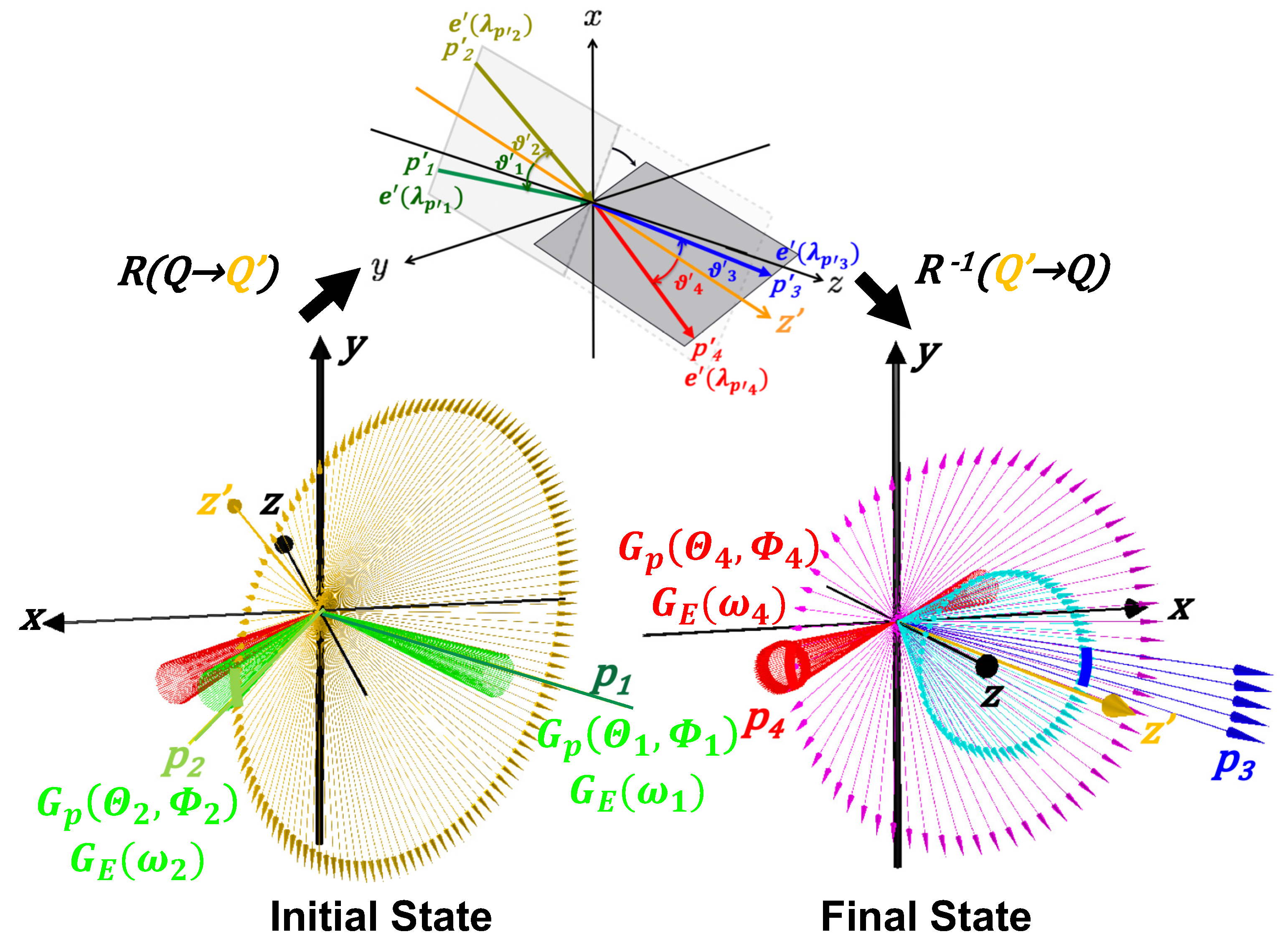Figure 4 illustrates the entire flow of the calculation. The left figure depicts the initial state of two scattering photons with incidence of two creation beams (green) and an inducing beam (red), while the right figure indicates the final state photons, that is, the inducing beam photons and signal photons (blue) in the laboratory coordinates by omitting the outgoing two creation beams. The top figure is to remind of the scattering amplitude calculation in the primed coordinates. Probability distribution functions in momentum space $G_p$ as a function of polar angles ${\Theta }_i$ and azimuthal angles ${\Phi }_i$ in the laboratory coordinates and those in energy $G_E\left({\omega }_i\right)$ for individual photons $i=1,2,4$ are assigned to individual focused beams by denoting the normalized Gaussian distributions as G. The actual steps for the calculations are as follows:

• Select a finite-size segment of $p_1$ from given $G_E\left({\omega }_1\right)G_p({\Theta }_1,{\Phi }_1)$ distributions.
• Find $p_2$ which satisfies the following resonance condition

  $$m_a=E_{cms}=2\sqrt{{\omega }_1{\omega }_2}sin\left(\frac{{\vartheta }_1+{\vartheta }_2}{2}\right)$$

  (18)

  with respect to the selected $p_1$ and to a finite energy segment in $G_E\left({\omega }_2\right)$ for a given mass parameter $m_a$. The possible $p_2$ candidates satisfying the resonance condition form the yellow thin cone around the $p_1$-axis reflecting the width of the Breit–Wigner function as shown in the left figure.
• Form a $z^{\prime }$-axis so that the pair transverse momentum, $p_T$, becomes zero, which is defined as zero-$p_T$ coordinates (primed coordinates) in contrast to the laboratory coordinates to which the three beams are physically mapped. Only a portion of the creation beam prepared for $p_2$ overlapping with the yellow cone can effectively contribute to the resonance production and, hence, the field weight for the pair can be eventually evaluated by properly reflecting $G_E\left({\omega }_1\right)G_p({\Theta }_1,{\Phi }_1)$ and $G_E\left({\omega }_2\right)G_p({\Theta }_2,{\Phi }_2)$.
• Convert the polarization vectors $e_i\left({\lambda }_i\right)$ as well as the momentum vectors from the laboratory coordinates to the zero-$p_T$ coordinates through the coordinate rotation $\mathcal{R}(Q\to Q^{\prime })$.
• The axial symmetric nature of possible final-state momenta $p_3^{\prime }$ and $p_4^{\prime }$ around $z^{\prime }$ is represented by the light-blue and magenta vectors in the right figure. A spontaneous scattering probability with the vertex factors using the primed polarization vectors in the planes containing the four photon wave vectors is calculated in the given zero-$p_T$ coordinates as illustrated in the top figure. By using the axial symmetric nature around $z^{\prime }$, the probability can be integrated over possible final state planes containing $p_3^{\prime }$ and $p_4^{\prime }$.
• In order to estimate the inducing effect for given $G_E\left({\omega }_4\right)G_p({\Theta }_4,{\Phi }_4)$ distributions fixed in the laboratory coordinates, a matching fraction of $p_4$ is calculated after rotating the primed vectors back to those in the laboratory coordinates from the zero-$p_T$ coordinates via the inverse rotation ${\mathcal{R}}^{-1}(Q^{\prime }\to Q)$. Based on the spread of $G_E\left({\omega }_4\right)$, the weights along the overlapping belt between the magenta and red vectors in the right figure are taken into account as the enhancement factor for the stimulation of the decay.
• Due to energy–momentum conservation, $p_3$ must balance with $p_4$. Thus a signal energy spread via ${\omega }_s\equiv {\omega }_3={\omega }_1+{\omega }_2-{\omega }_4$ and also the polar-azimuthal angle spreads by taking the $G_E\left({\omega }_4\right)G_p({\Theta }_4,{\Phi }_4)$ distributions into account are automatically determined. The volume-wise interaction rate ${\overline{\Sigma }}_I$ is then integrated over the inducible solid angle of $p_3$ reflecting all the energy and angular spreads included in the focused three beams.
• With Equation (8) the signal yield ${\mathcal{Y}}_{c+i}$ can be evaluated.

3. Expected Sensitivity

We evaluate search sensitivities based on the concept of a three-beam stimulated resonant photon collider (${}^{\mathrm{t}}$SRPC) with variable incident angles for scanning ALP masses around the eV range as illustrated in Figure 1. By assuming high-intensity femtosecond lasers such as Titanium:Sapphire lasers with 1 J pulse energy for simplicity, we consider that two identical creation beams with the central photon energy ${\omega }_c$ and the time duration ${\tau }_c$ are symmetrically incident with the same beam incident angle ${\theta }_c$ and an inducing laser with the central photon energy ${\omega }_i\equiv u{\omega }_c$ with $0<u<1$ is incident with the corresponding angle which satisfies energy–momentum conservation by requiring a common signal photon energy $(2-u){\omega }_c$ independent of various incident angle combinations. The central wavelength is around 800 nm and then we assume the ability to produce high harmonic waves from the fundamental wavelength for creation beams and to generate an inducing beam with a non-integer number u based on the optical parametric amplification (OPA) technique in order to discriminate signal waves against the integer number high harmonic waves originating from the creation beams. Since the OPA technique cannot achieve the perfect conversion from the fundamental wavelength, we assume 0.1 J pulse energy and also the elongation of the pulse duration for the inducing beam compared to that in the creation beam.

Table 1. Experimental parameters used to numerically calculate the upper limits on the coupling–mass relations.

Parameter	Value
Central wavelength of creation laser ${\lambda }_c$	800 nm ($\omega$)/400 nm ($2\omega$)/267 nm (3$\omega$)
Relative linewidth of creation laser, $\delta {\omega }_c/<{\omega }_c>$	${10}^{-2}$
Duration time of creation laser, ${\tau }_c$	30 fs
Creation laser energy per ${\tau }_c$, $E_c$	1 J
Number of creation photons ($\omega$), $N_c$	$4.03\times {10}^{18}$ photons
Number of creation photons ($2\omega$), $N_c$	$2.01\times {10}^{18}$ photons
Number of creation photons ($3\omega$), $N_c$	$1.34\times {10}^{18}$ photons
Beam diameter of creation laser beam, $d_c$	60 mm
Polarization	linear (P-polarized state)
Central wavelength of inducing laser, ${\lambda }_i$	1300 nm
Relative linewidth of inducing laser, $\delta {\omega }_i/<{\omega }_i>$	${10}^{-2}$
Duration time of inducing laser beam, ${\tau }_i$	100 fs
Inducing laser energy per ${\tau }_i$, $E_i$	$0.1$ J
Number of inducing photons, $N_i$	$6.54\times {10}^{17}$ photons
Beam diameter of inducing laser beam, $d_i$	30 mm
Polarization	circular (left-handed state)
Focal length of off-axis parabolic mirror, $f_c=f_i$	600 mm
Overall detection efficiency, $ϵ$	1%
Number of shots, $N_{shots}$	${10}^5$ shots
$\delta N_S$	100

summarizes assumed parameters for two identical creation laser beams and an including laser beams as well as the common focusing and statistical parameters.

Given a set of three-beam laser parameters P in Table 1, the number of stimulated signal photons, $N_{obs}$, is expressed as

$$N_{obs}={\mathcal{Y}}_{c+i}(m_a,g/M;P)N_{shot}ϵ,$$

(19)

which is a function of ALP mass $m_a$ and coupling $g/M$, where $N_{shot}$ the number of laser shots and $ϵ$ the overall efficiency of detecting $p_3$. For a set of $m_a$ values with an assumed $N_{obs}$, a set of coupling $g/M$ can be estimated by numerically solving Equation (19).

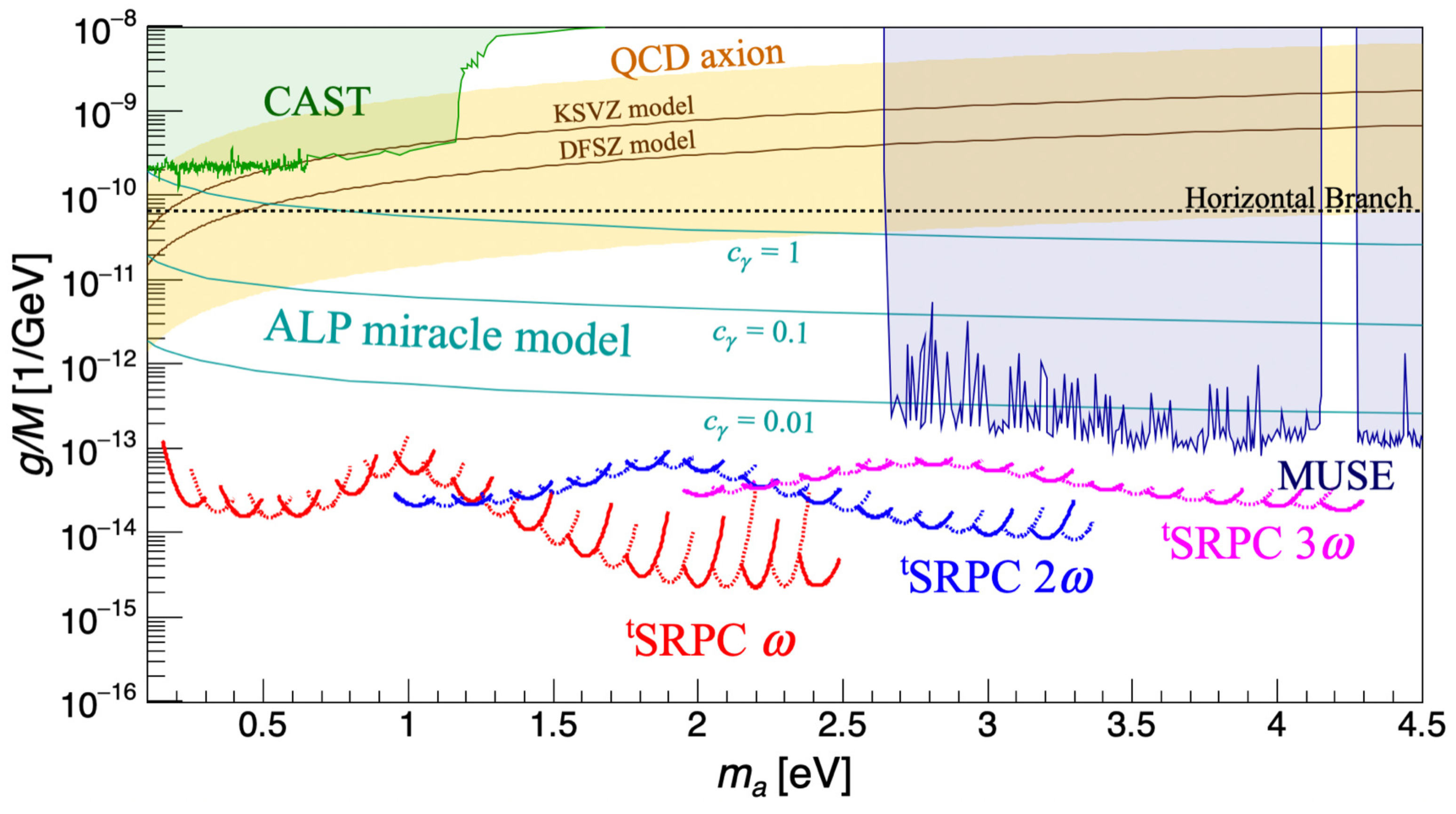
Based on parameters in Table 1, Figure 5 shows the reachable sensitivities in the coupling–mass relation for the pseudoscalar field exchange at a 95% confidence level by ${}^{\mathrm{t}}$SRPC. The red, blue and magenta solid/dashed curves show the expected upper limits by ${}^{\mathrm{t}}$SRPC when we assume ${\omega }_c=800$ nm (fundamental wavelength $\omega$), 400 nm (second harmonic $2\omega$) and 267 nm (third harmonic $3\omega$), respectively. The ALP mass scanning is assumed to be performed with the step of $0.1$ eV. Thanks to energy and momentum fluctuations at around the focal point, the same order sensitivities are maintained within the assumed scanning step (the local minima of the parabolic behavior in the coupling correspond to different incident angle setups in Figure 5). For easy viewing, the solid and dashed curves are drawn alternatively. These assumed photon sources are all available within the current technology [18] in terms of the photon wavelength and energy per pulse.

These sensitivity curves are obtained based on the following condition. In this virtual search, the null hypothesis is supposed to be fluctuations on the number of photon-like signals following a Gaussian distribution whose expectation value, $\mu$, is zero for the given total number of collision statistics. The photon-like signals implies a situation where photons-like peaks are counted by a peak finder based on digitized waveform data from a photodevice [11], where electrical fluctuations around the baseline of a waveform cause both positive and negative numbers of photon-like signals. In order to exclude this null hypothesis, a confidence level $1-\alpha$ is introduced as

$$1-\alpha =\frac{1}{\sqrt{2\pi }\sigma }{\int }_{\mu -\delta }^{\mu +\delta }{e}^{-{(x-\mu )}^2/\left(2{\sigma }^2\right)}dx=\mathrm{erf}\left(\frac{\delta }{\sqrt{2}\sigma }\right),$$

(20)

where $\mu$ is the expected value of an estimator x following the hypothesis, and $\sigma$ is one standard deviation. In this search, the estimator x corresponds to the number of signal photons $N_S$ and we assume the detector-acceptance-uncorrected uncertainty $\delta N_S$ as the one standard deviation $\sigma$ around the mean value $\mu =0$. For setting a confidence level of 95%, $2\alpha =0.05$ with $\delta =2.24\sigma$ is used, where a one-sided upper limit by excluding above $x+\delta$ [19] is considered. For a set of experimental parameters P in Table 1, the upper limits on the coupling–mass relation, $m_a$ vs. $g/M$, are then estimated by numerically solving the following equation

$$N_{obs}=2.24\delta N_S={\mathcal{Y}}_{c+i}(m_a,g/M;P)N_{shots}ϵ.$$

(21)

The horizontal dotted line shows the upper limit from the Horizontal Branch (HB) observation [20]. The purple area shows bounds by the optical MUSE-faint survey [21]. The green area is excluded by the helioscope experiment CAST [22]. The yellow band shows the QCD axion benchmark models with $0.07<|E/N-1.95|<7$ where KSVZ($E/N=0$) [4,5] and DFSZ($E/N=8/3$) [23] are shown with the brawn lines. The cyan lines show predictions from the ALP miracle model [6] with its intrinsic model parameters $c_{\gamma }=1.0$, $0.1,0.01$, respectively.

4. Conclusions

We have evaluated expected sensitivities to axion-like particles coupling to photons based on the concept of a three-beam stimulated resonant photon collider with focused short-pulse lasers. Within the current high-intensity laser technology reaching the pulse energy 1 J, we found that the searching method can probe ALPs in the eV mass range down to $g/M=\mathcal{O}\left({10}^{-14}\right)$ GeV⁻¹. This sensitivity is sufficient to test the unexplored domain motivated by the miracle model as well as the benchmark QCD axion models.