Abstract
This paper studies dispersive bright and dark optical solitons, modeled by the Schrödinger–Hirota equation, numerically by the aid of the Adomian decomposition. The surface plots of the algorithm yielded an impressively small measure. The effects of soliton radiation are ignored.
1. Introduction
There are multiple models that study the dynamics of dispersive optical solitons that propagate through an optical fiber. A few such models are the Fokas–Lenells equation, cubic-quartic solitons; pure-quartic solitons, pure-cubic solitons, and highly dispersive solitons. The Schrödinger–Hirota equation (SHE) will be used to explain the dynamics of dispersive optical solitons in today’s presentation. This equation is derived from the main governing equation that is studied in nonlinear optics, namely the nonlinear Schrödinger’s equation (NLSE) in the presence of a third-order dispersion and other Hamiltonian type perturbations. To derive SHE, one needs to apply Lie transform to the NLSE and ignore the higher order terms which would eventually lead to SHE. This derivation has been discussed previously [1]. The nonlinear form of the refractive index that would be taken into consideration is the Kerr type that is alternatively known as the cubic type. Additional research work related to the present study can be found in [2,3,4].
This work is a numerical study of SHE that is conducted using the Adomian decomposition method (ADM). To this effect, SHE is first split into three operators, namely the temporal derivative, the linear operator, and the nonlinear operator. Subsequently, the Adomian polynomials are constructed. Finally, the Laplace transform is carried out for each of the components and then added. The final solution structure is obtained by taking the inverse Laplace transform recursively for each component and taking its N-component finite sum. The test examples were carried out for both bright and dark solitons. It must be noted that the adverse effect such as soliton radiation as well as the slow-down effect of solitons are neglected here so that the focus is on the core soliton. The error plots were finally constructed and gave an impressive error measure that is of the order of . The detailed scheme and the soliton surface plots are discussed in the subsequent sections of this manuscript.
2. Schrödinger–Hirota Equation
The Schrödinger–Hirota equation (SHE) with Kerr law nonlinearity in dimensionless form is written as [1,5,6,7,8,9,10]:
where stands for the complex-valued wave profile and is its linear temporal evolution. Furthermore, in Equation (1) a represents the group velocity dispersion (GVD), c is the Kerr law nonlinearity coefficient, is the coefficient of third order dispersion (3OD), is the coefficient of nonlinear dispersion and i is the imaginary unit. The dynamics of dispersive optical solitons propagating over long-range optical fibers are modeled by Equation (1), such as the ones used for inter-oceanic or intercontinental telecommunications.
3. Bright and Dark Solitons for the Governing Equation (1)
3.1. Bright Solitons
3.2. Dark Solitons
4. The Laplace Transform Combined with the Adomian Decomposition Method
In this section we will briefly develop the well-known Adomian decomposition method and demonstrate its improvement resulting from the method’s combination with the Laplace transform [12,13]. The development is focused on achieving both bright and dark solitons for the SHE model (1).
In general, using operators we can write Equation (1) as
subject to the initial condition
where is the usual time derivation operator, is a linear differential operator, which in our case turns out to be
while is a nonlinear operator, which acts as a
According to the standard Adomian decomposition method, the solution q can be expanded in an infinite series as follows:
and the nonlinear term series
where each of the is an Adomian polynomial [14].
In the case of the nonlinear operator given in Equation (15), we can decompose it as
where
both and can be decomposed into infinite series of Adomian polynomials given by:
where as symbolizes the Adomian polynomials, which will be calculated by means of the formulas established in [15], that is,
and
From now on will denote the Laplace transform and its inverse operator. Then applying on both sides of the operational Equation (12) we have
and making use of the initial condition, which will be derived from the initials profiles of the solitons f, we obtain
Substituting Equations (16)–(17) into Equation (25) gives
Considering the process of decomposition in the Adomian polynomials (18)–(21) we obtain
Matching both sides of Equation (27), we obtain the Laplace transform of each of the components of the solution, that is
and for every , the recursive relations are given by
Now let us compute some Adomian polynomials, for this purpose let us consider the nonlinear operators and on q appearing in Equation (19) and by using formulas (22) and (23), we obtain
and so on for other Adomian polynomials.
Finally, considering the inverse Laplace transform , the components , , , …, are then determined recursively by:
where is referred to as the zero-th component.
Now, the solution functions q in the Laplace-Adomian decomposition algorithm are extracted as
Convergence of the Algorithm
The solution given above is a series that quickly and uniformly converges to the exact solution. To validate the convergence of the series (31), we will employ a strong important functional analysis result. For sufficient convergence conditions of the proposed technique, we demonstrate the following theorem and its application in the previous algorithm.
Theorem 1.
Letbe a Banach space andbe a contractive nonlinear operator such that for all, , . Consequently, using the Banach contraction principle, T has a unique point x such that.
The series presented in (31) may be expressed using the Adomian decomposition technique as follows:
and assume that where , therefore, we have
- (a)
- ,
- (b)
Proof.
To prove (a), by the first step of mathematical induction, i.e., if , we have
Now suppose that the result is true for , then
we have
Therefore, we have
hence it follows that .
To prove (b), according to the fact that and that also . Therefore, we have
wich implies that
For the above, the term approximate solution of the power series (31) is given by
For more details about the convergence of the method, see [16,17,18]. □
In the next section, we will perform the numerical simulation for the calculation of optical solitons for Equation (1) in order to show the high degree of accuracy and efficiency of the algorithm obtained from LADM.
5. Numerical Simulations of Solitons for Equation (1)
The numerical simulation results are carried out by using the Mathematica software and the results obtained will be shown graphically.
5.1. Bright Highly Dispersive Optical Soliton
We now consider the initial condition at from Equation (2):
We will carry out the simulation for three cases with the parameters given in Table 1 and the results obtained are shown graphically in Figure 1, Figure 2 and Figure 3.

Table 1.
Coefficients of Equation (1) to simulate bright solitons.
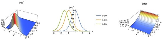
Figure 1.
3D, 2D and absolute error graphics for Case 1.
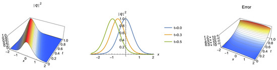
Figure 2.
3D, 2D and absolute error graphics for Case 2.
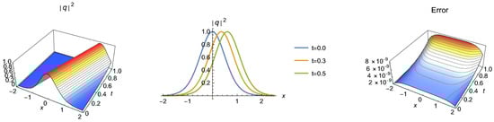
Figure 3.
3D, 2D and absolute error graphics for Case 3.
5.2. Dark Highly Dispersive Optical Soliton
We now consider the initial condition at from Equation (7):
We will carry out the simulation for three cases with the parameters given in Table 2 the results obtained are shown graphically in Figure 4, Figure 5 and Figure 6.
Table 2.
Coefficients of Equation (1) to simulate dark solitons.
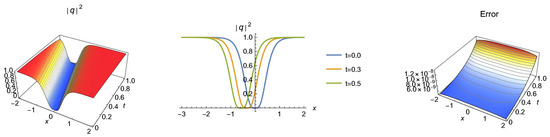
Figure 4.
3D, 2D and absolute error graphics for Case 4.
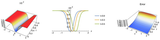
Figure 5.
3D, 2D and absolute error graphics for Case 5.
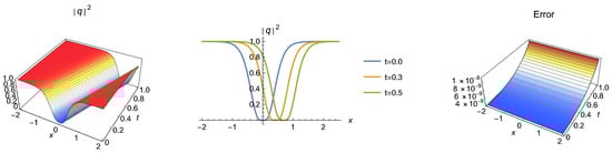
Figure 6.
3D, 2D and absolute error graphics for Case 6.
6. Conclusions
The results of the current paper display a visual effect of the dynamics of dispersive optical solitons that emerge from SHE. In this context, both bright and dark solitons are taken into consideration. Dispersive bright and dark optical solitons are modeled in this paper by using SHE with the Kerr law of nonlinear refractive index change, and these solitons are simulated numerically. The scheme is from the Laplace ADM algorithm that is presented. The error measure is impressively small which enabled the display of almost perfect surface plots of these solitons. The effects of soliton radiation are not included and thus the slow-down of solitons due to third-order dispersive effects is not reflected in the numerical schemes.
This work and the results presented here pave the way for future research to take place. These are to be extended to birefringent fibers, followed by an extension to DWDM topology. These simulations are in the work and the results will be subsequently and sequentially disseminated. Another feature to think about is the formation of quiescent solitons that come from the fact that the CD is rendered to be nonlinear for SHE. This aspect will be reported on further down the road.
Author Contributions
Conceptualization, A.B.; writing—original draft preparation, O.G.-G.; project administration, L.M.; project administration, S.M. All authors have read and agreed to the published version of the manuscript.
Funding
This research received no external funding.
Institutional Review Board Statement
Not applicable.
Informed Consent Statement
Not applicable.
Data Availability Statement
Not applicable.
Acknowledgments
This work was supported by the project “DINAMIC”, Contract no. 12PFE/2021.162. The authors are extremely thankful for it.
Conflicts of Interest
The authors declare no conflict of interest.
References
- Biswas, A.; Jawad, A.J.M.; Manrakhan, W.N.; Sarma, A.K.; Khan, K.R. Optical solitons and complexitons of the Schrödinger-Hirota equation. Opt. Laser Technol. 2012, 44, 2265–2269. [Google Scholar] [CrossRef]
- Khamis, A.K.; Lotfy, K.; El-Bary, A.A.; Mahdy, A.M.S.; Ahmed, M.H. Thermal-piezoelectric problem of a semiconductor medium during photo-thermal excitation. Waves Random Complex Media 2021, 31, 2499–2513. [Google Scholar] [CrossRef]
- Mahdy, A.M.S.; Lotfy, K.; Ismail, E.A.; El-Bary, A.; Ahmed, M.; El-Dahdouh, A.A. Analytical solutions of time-fractional heat order for a magneto-photothermal semiconductor medium with Thomson effects and initial stress. Results Phys. 2020, 18, 103174. [Google Scholar] [CrossRef]
- Koyunbakan, H. The transmutation method and Schrödinger equation with perturbed exactly solvable potential. J. Comput. Acoust. 2009, 17, 1–10. [Google Scholar] [CrossRef]
- Bhrawy, A.H.; Alshaery, A.A.; Hilal, E.M.; Manrakhan, W.N.; Savescu, M.; Biswas, A. Dispersive optical solitons with Schrödinger-Hirota equation. J. Nonlinear Opt. Phys. Mater. 2014, 23, 1450014. [Google Scholar] [CrossRef]
- Bernstein, I.; Zerrad, E.; Zhou, Q.; Biswas, A.; Melikechi, N. Dispersive optical solitons with Schrödinger-Hirota equation by traveling wave hypothesis. Optoelectron. Adv.-Mater.-Rapid Commun. 2015, 9, 792–797. [Google Scholar]
- Kaur, L.; Wazwaz, A.M. Bright-dark optical solitons for Schrödinger-Hirota equation withvariable coefficients. Optik 2019, 179, 479–484. [Google Scholar] [CrossRef]
- Huang, W.-T.; Zhou, C.-C.; Lü, X.; Wang, J.-P. Dispersive optical solitons for the Schrödinger-Hirota equation in optical fibers. Mod. Phys. Lett. B 2021, 35, 2150060. [Google Scholar] [CrossRef]
- Chowdury, A.; Ankiewicz, A.; Akhmediev, N. Moving breathers and breather-to-soliton conversions for the Hirota equation. Proc. R. Soc. A 2015, 471, 20150130. [Google Scholar] [CrossRef]
- Bakodah, H.O.; Banaja, M.A.; Alshaery, A.A.; Al Qarni, A.A. Numerical solution of dispersive optical solitons with Schrödinger-Hirota equation by improved Adomian decomposition method. Math. Probl. Eng. 2019, 2019, 2960912. [Google Scholar] [CrossRef]
- Biswas, A.; Yildirim, Y.; Yasar, E.; Zhou, Q.; Alshomrani, A.S.; Moshokoa, S.P.; Belic, M. Dispersive optical solitons with Schrödinger-Hirota model by trial equation method. Optik 2018, 162, 35–41. [Google Scholar] [CrossRef]
- Adomian, G.; Rach, R. On the solution of nonlinear differential equations with convolution product nonlinearities. J. Math. Anal. Appl. 1986, 114, 171–175. [Google Scholar] [CrossRef]
- Adomian, G. Solving Frontier Problems of Physics: The Decomposition Method; Kluwer: Boston, MA, USA, 1994. [Google Scholar]
- Mohammed, A.S.H.F.; Bakodah, H.O. Numerical investigation of the Adomian-based methods with w-shaped optical solitons of Chen-Lee-Liu equation. Phys. Scr. 2021, 96, 035206. [Google Scholar] [CrossRef]
- Duan, J.-S. Convenient analytic recurrence algorithms for the Adomian polynomials. Appl. Math. Comput. 2011, 217, 6337–6348. [Google Scholar] [CrossRef]
- Cherruault, Y. Convergence of Adomian’s method. Kybernetes 1989, 18, 31–38. [Google Scholar] [CrossRef]
- Hosseini, M.M.; Nasabzadeh, H. On the convergence of Adomian decomposition method. Appl. Math. Comput. 2006, 182, 536–543. [Google Scholar] [CrossRef]
- Babolian, E.; Biazar, J. On the order of convergence of Adomian method. Appl. Math. Comput. 2002, 130, 383–387. [Google Scholar] [CrossRef]
Disclaimer/Publisher’s Note: The statements, opinions and data contained in all publications are solely those of the individual author(s) and contributor(s) and not of MDPI and/or the editor(s). MDPI and/or the editor(s) disclaim responsibility for any injury to people or property resulting from any ideas, methods, instructions or products referred to in the content. |
© 2022 by the authors. Licensee MDPI, Basel, Switzerland. This article is an open access article distributed under the terms and conditions of the Creative Commons Attribution (CC BY) license (https://creativecommons.org/licenses/by/4.0/).