Statistical Properties of X-ray Flares in Gamma-ray Bursts


Abstract
1. Introduction
2. Sample Selection and Data Analysis
3. Statistical Properties of the X-ray Flares
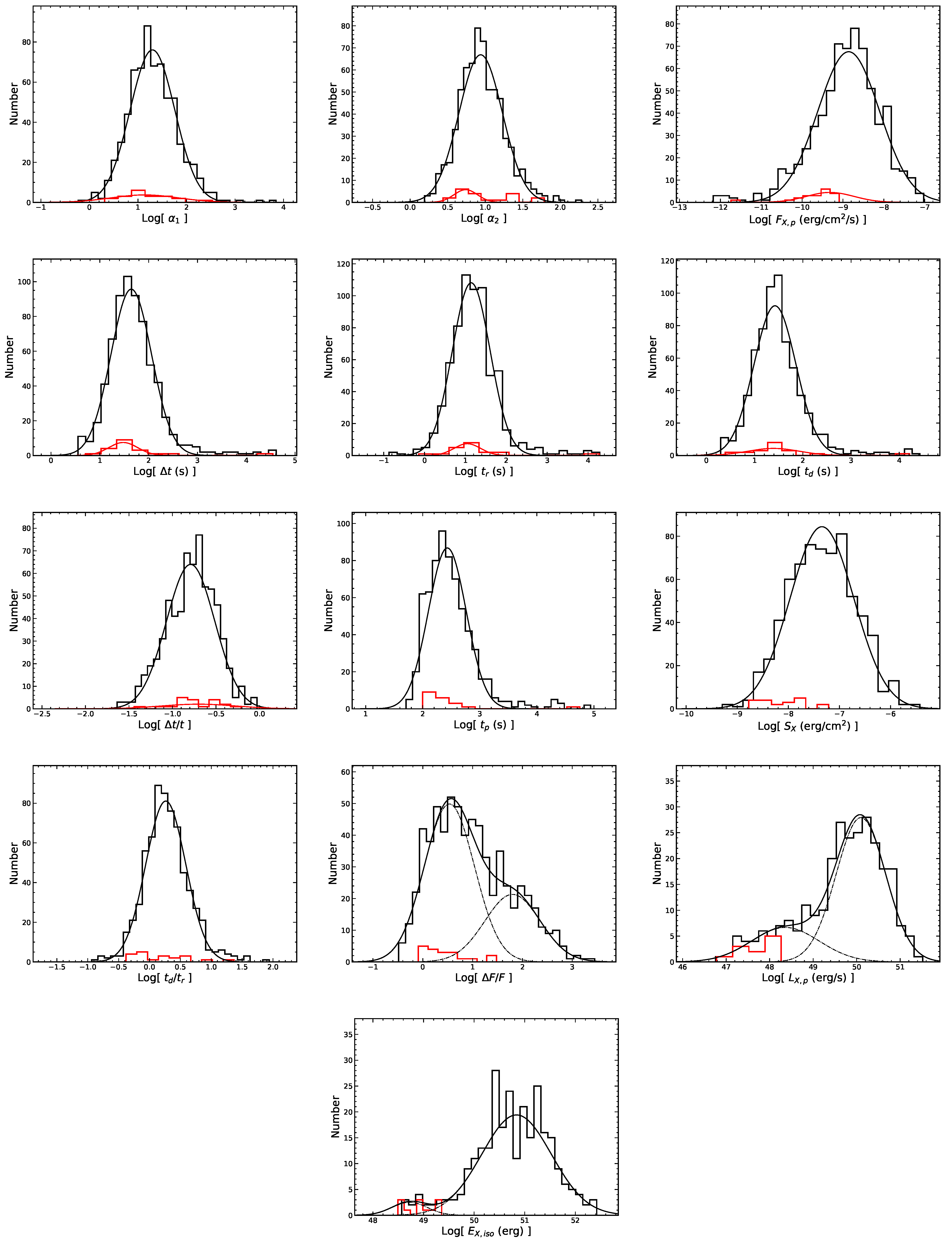
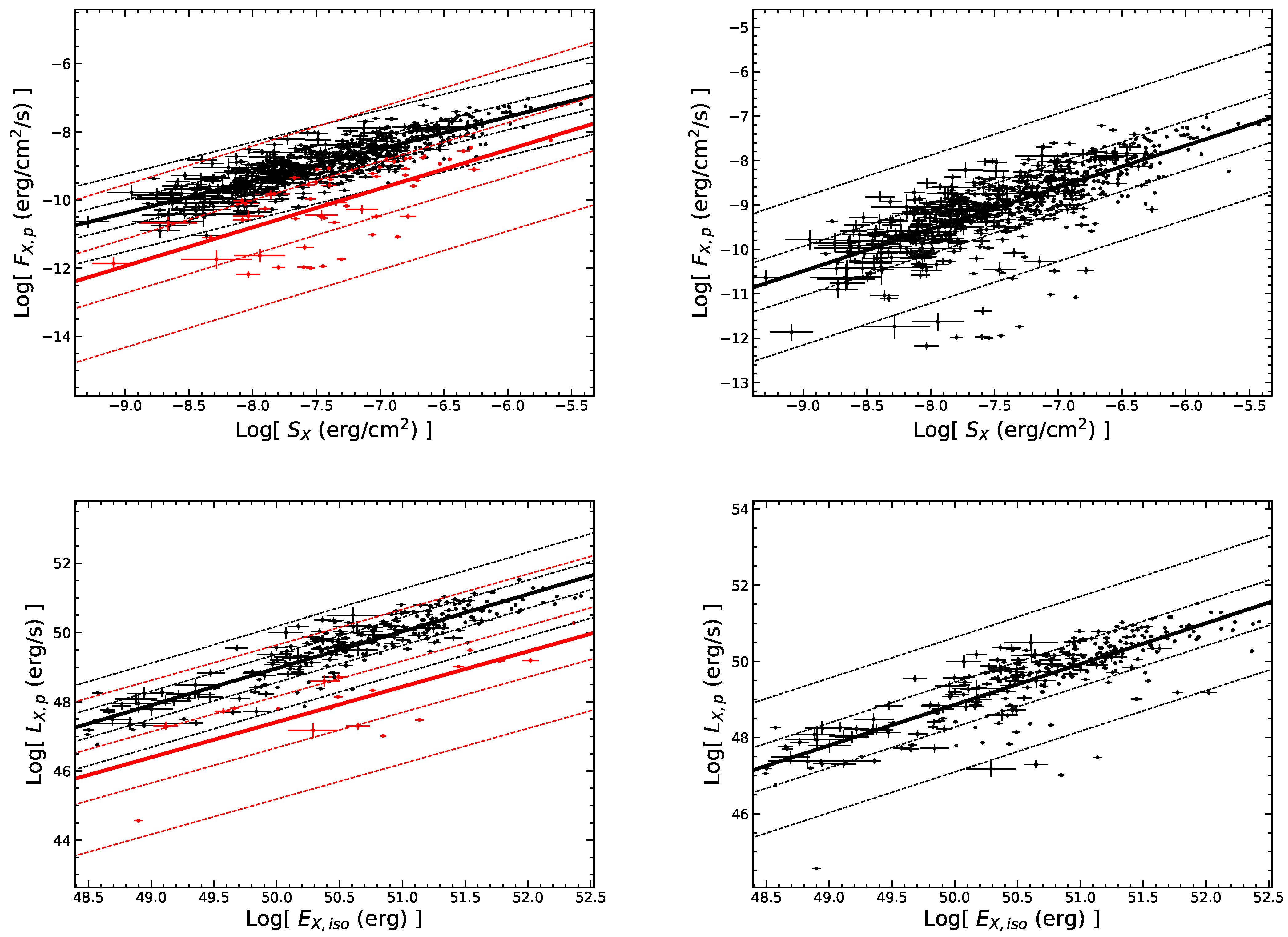
3.1. Distributions of Flare Parameters
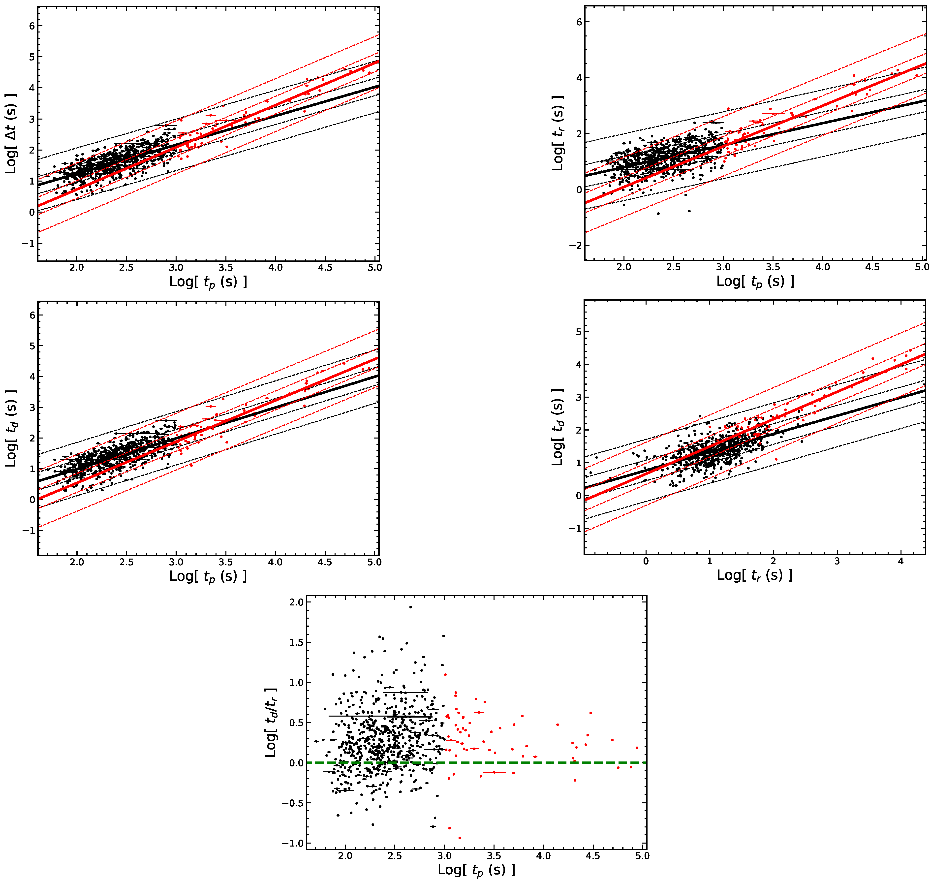
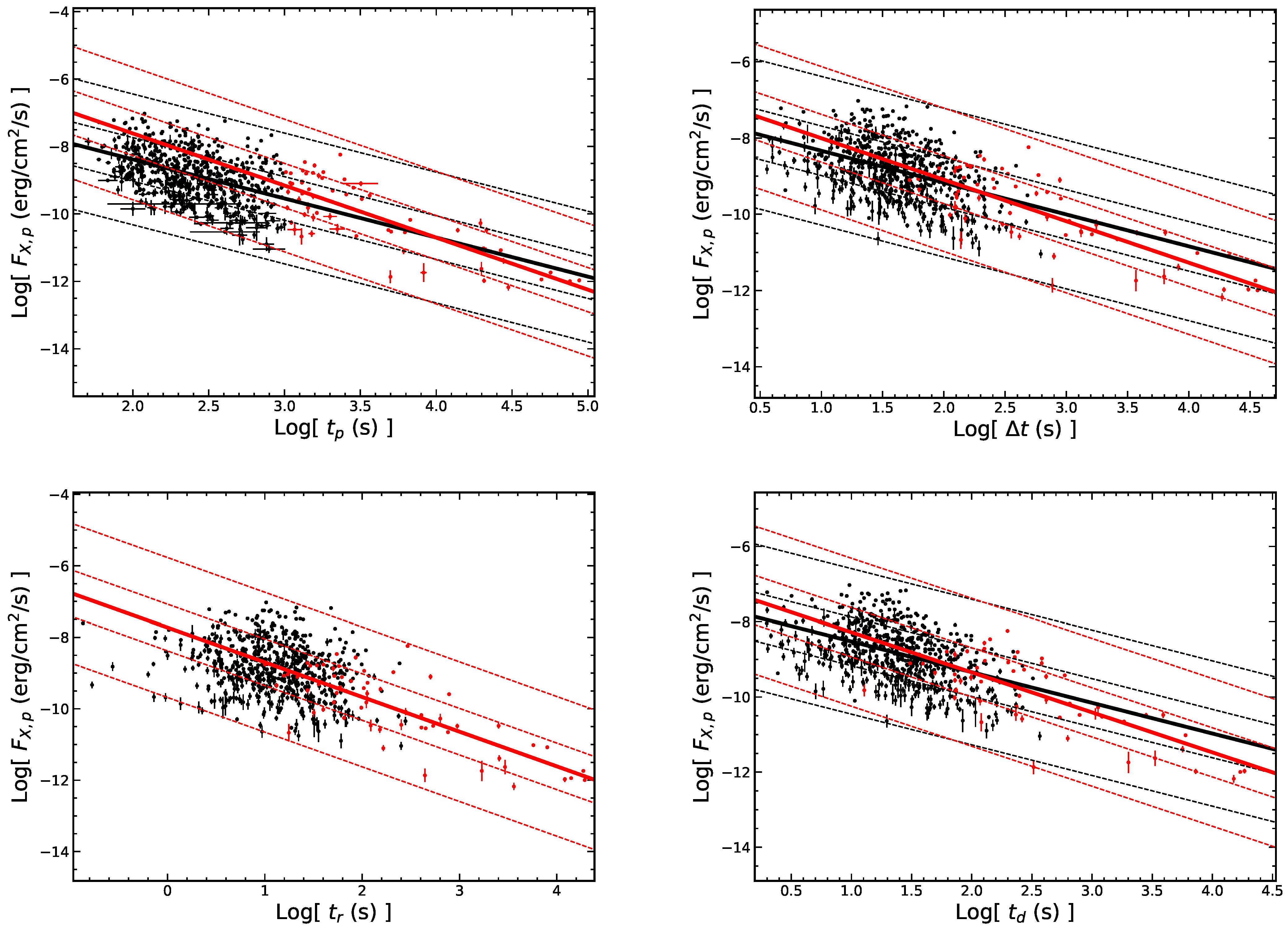
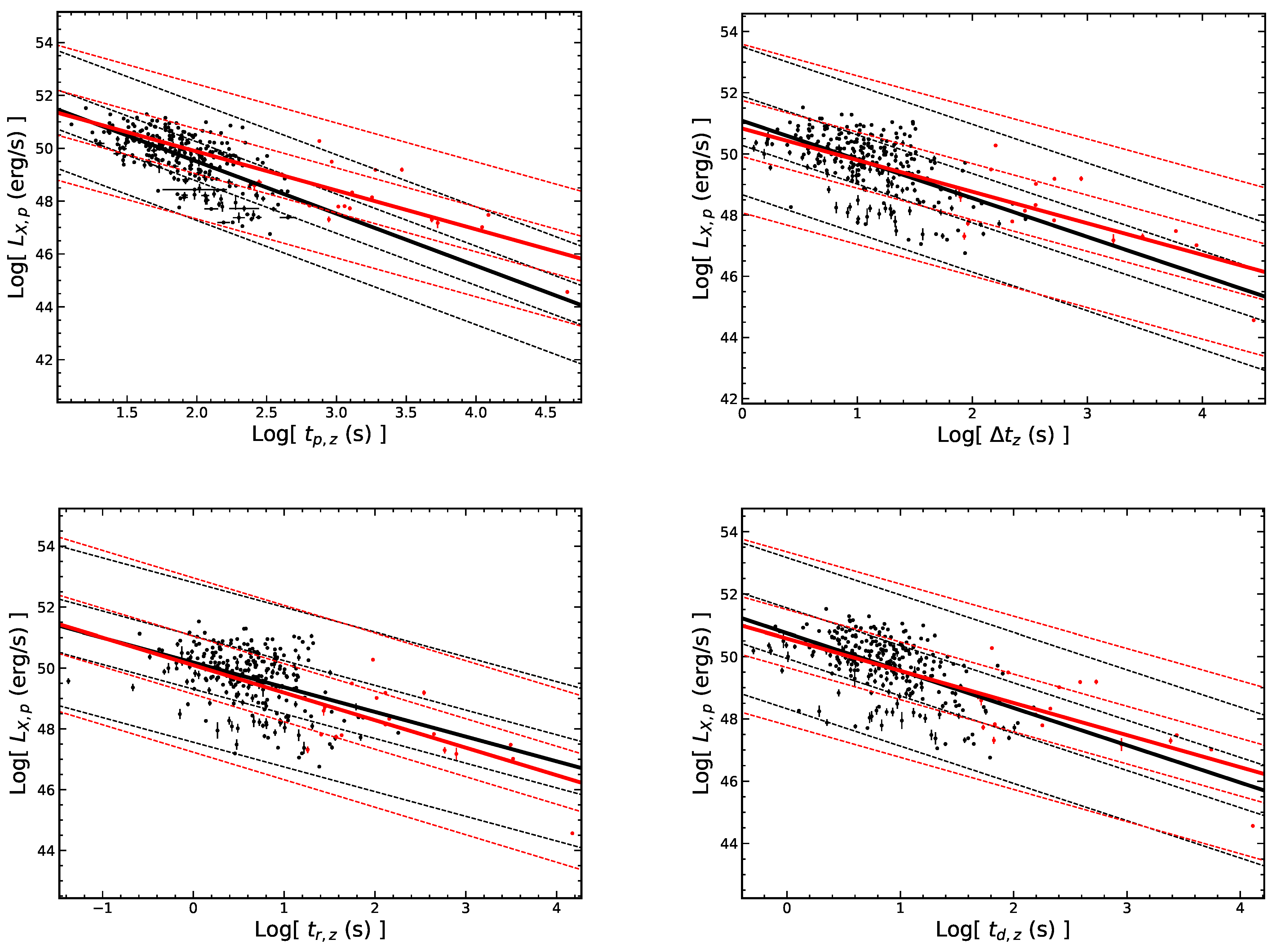
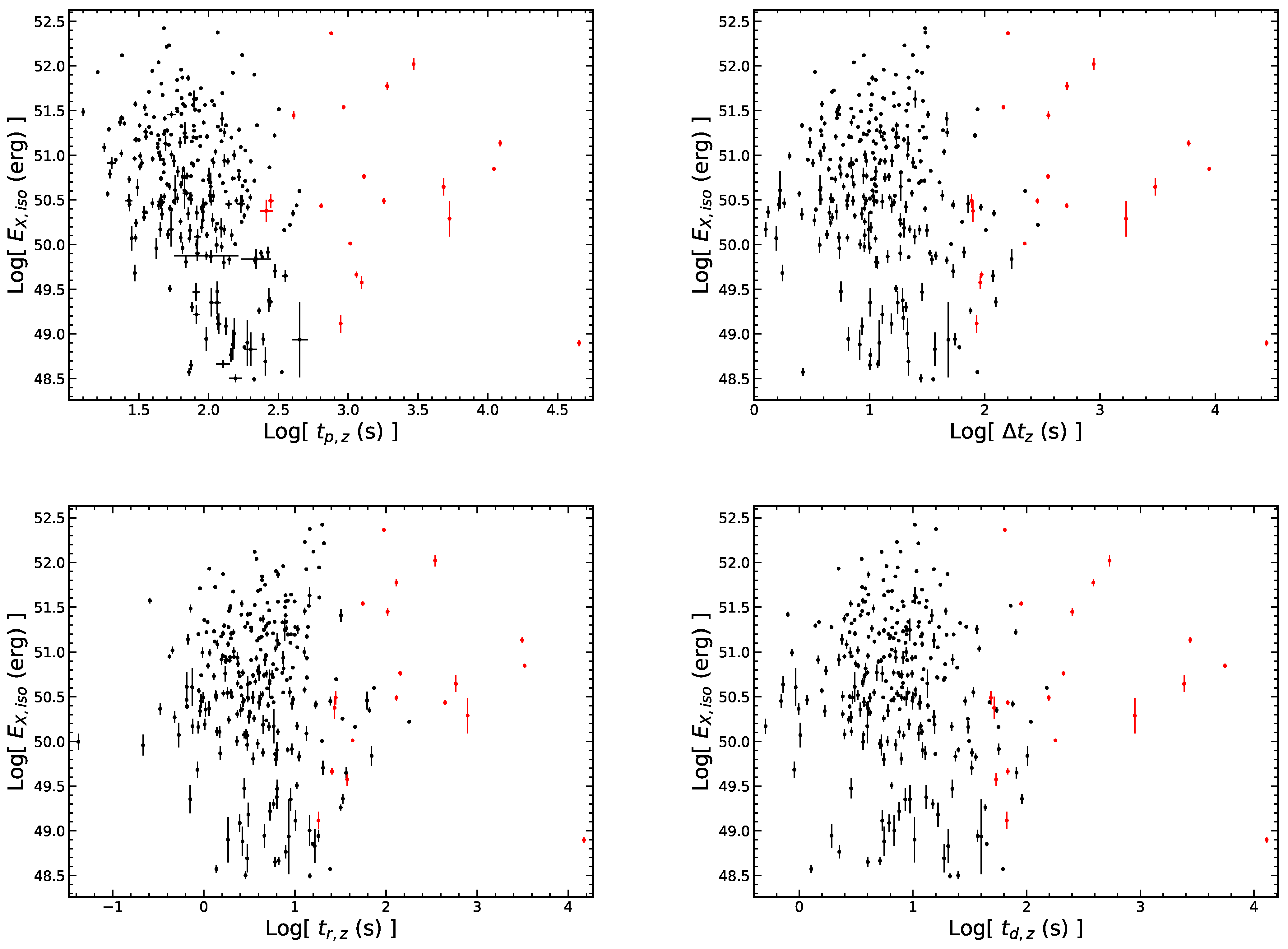
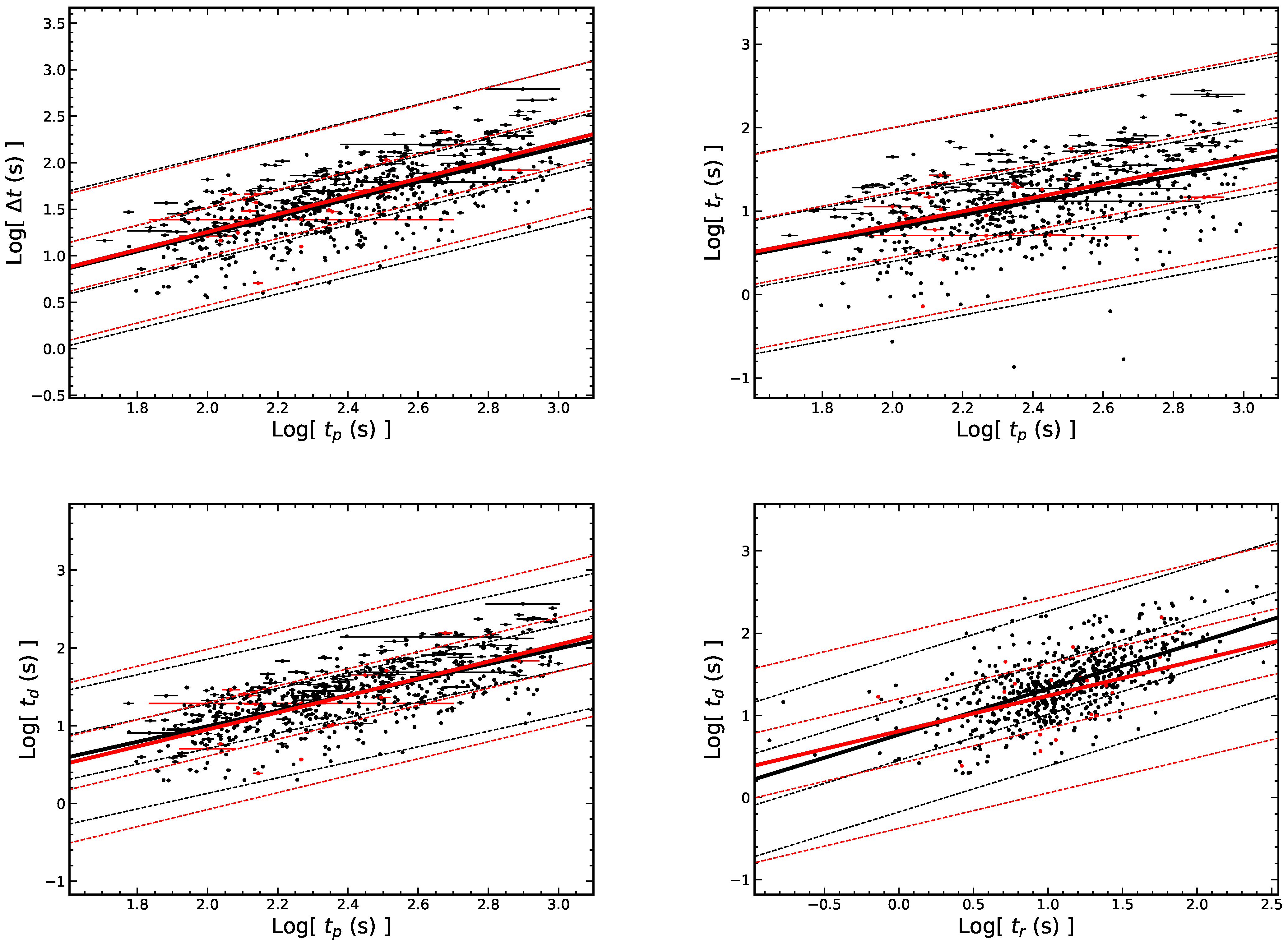
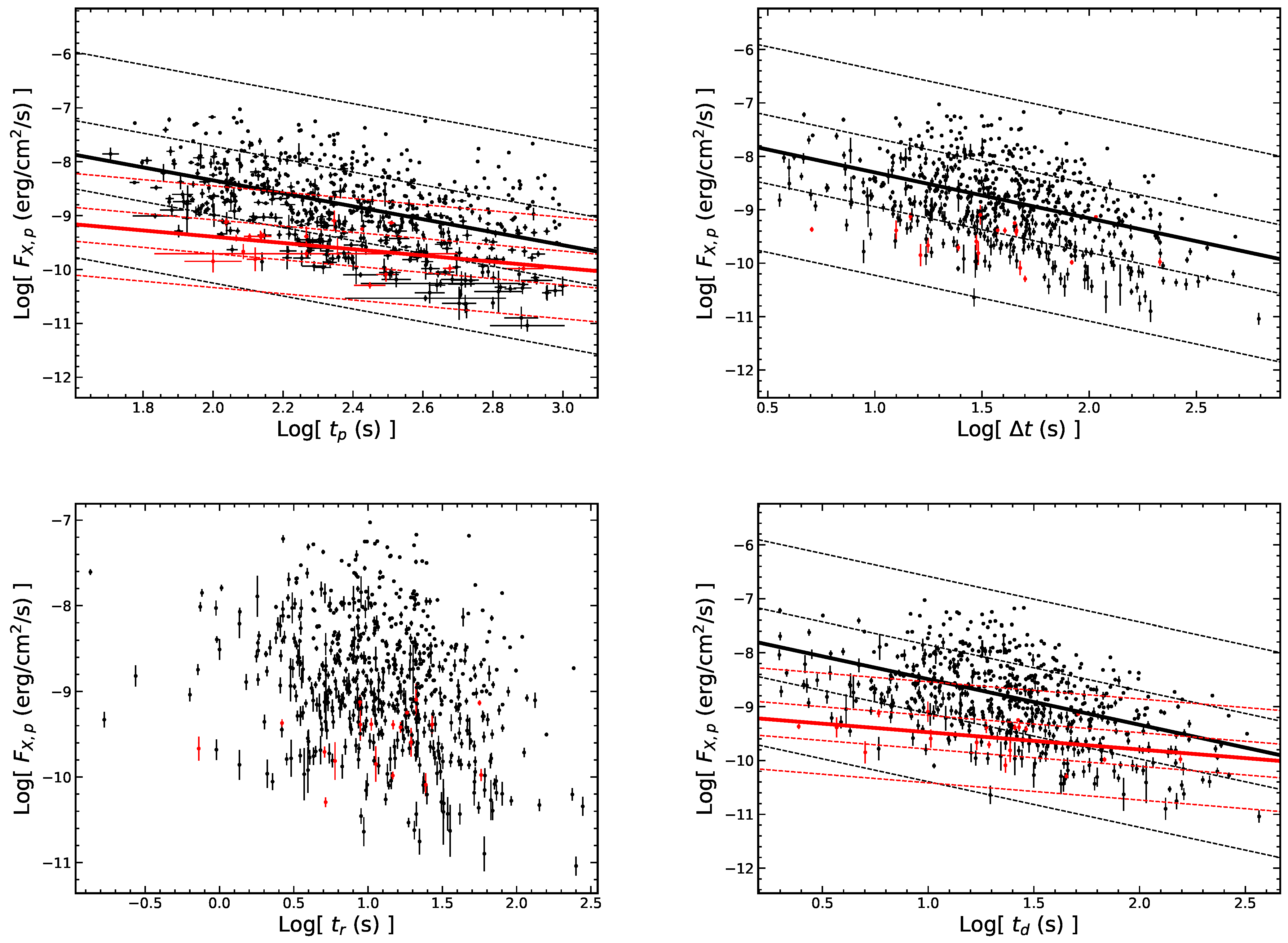
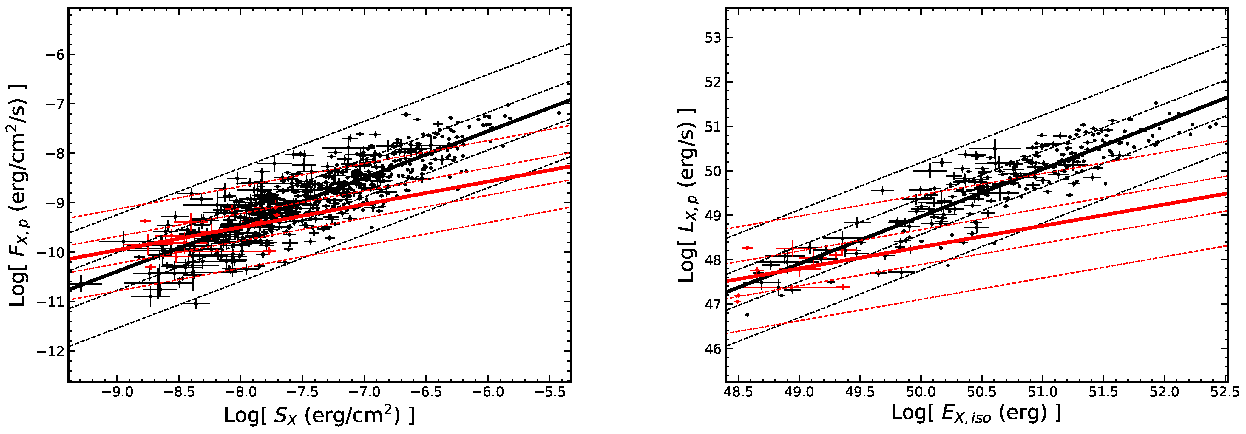
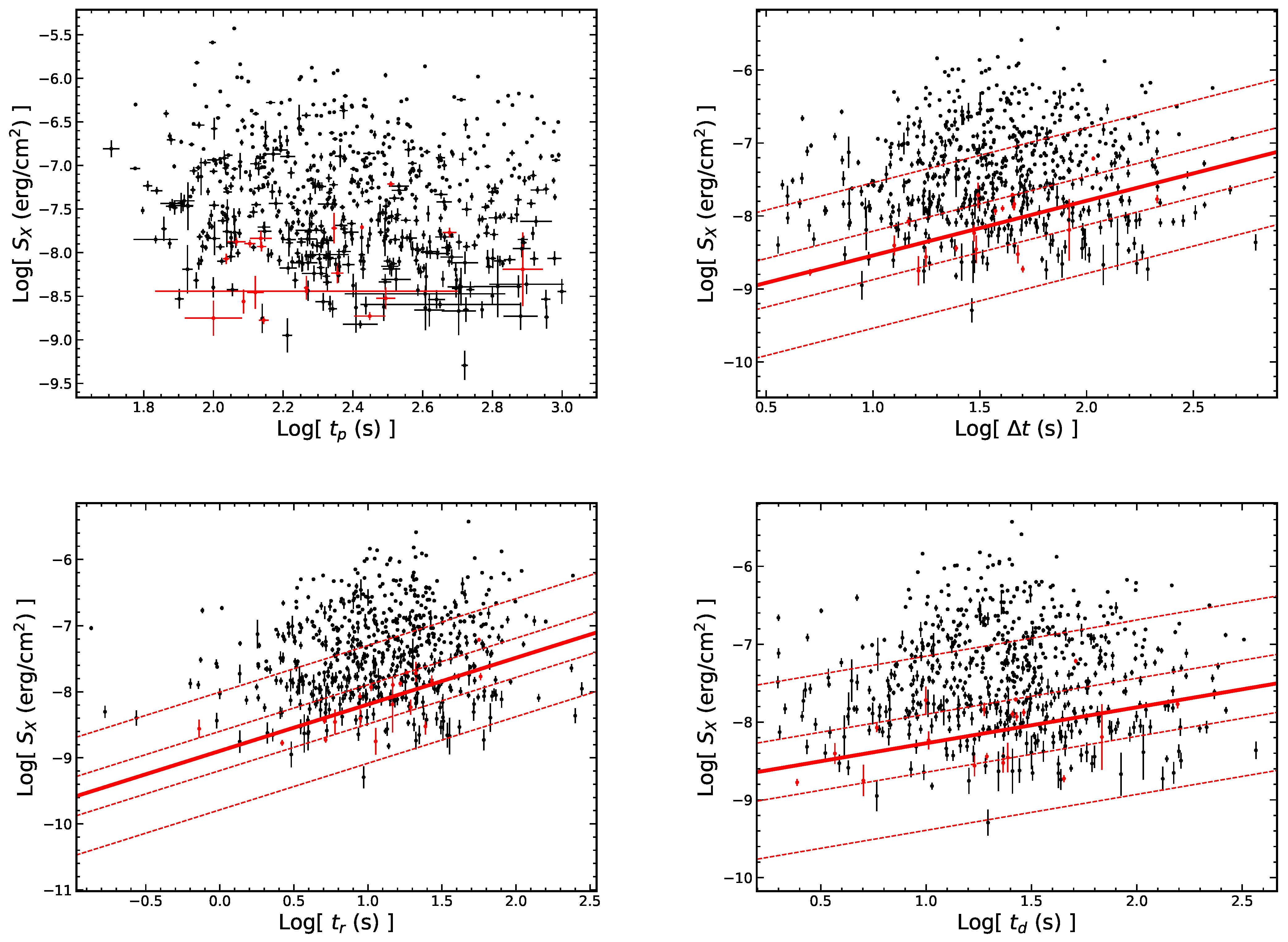
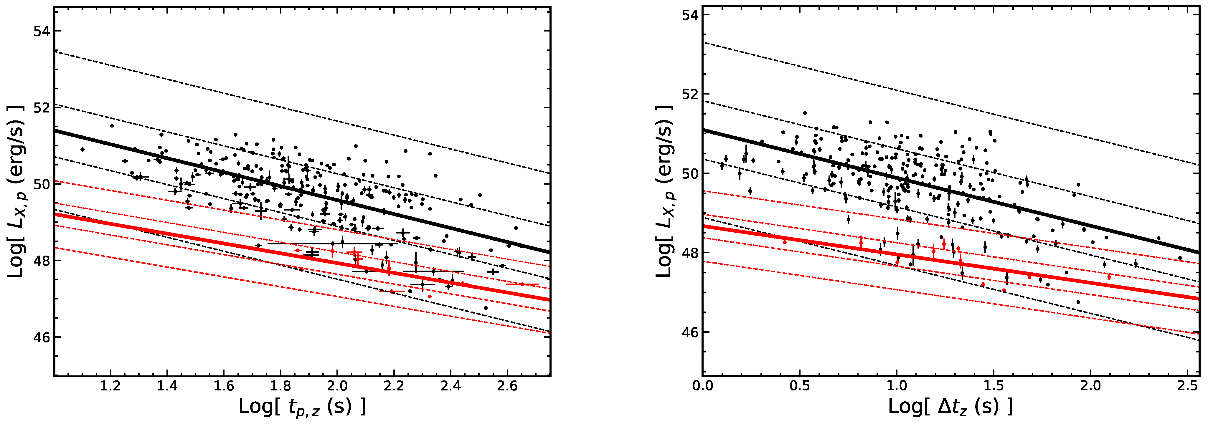
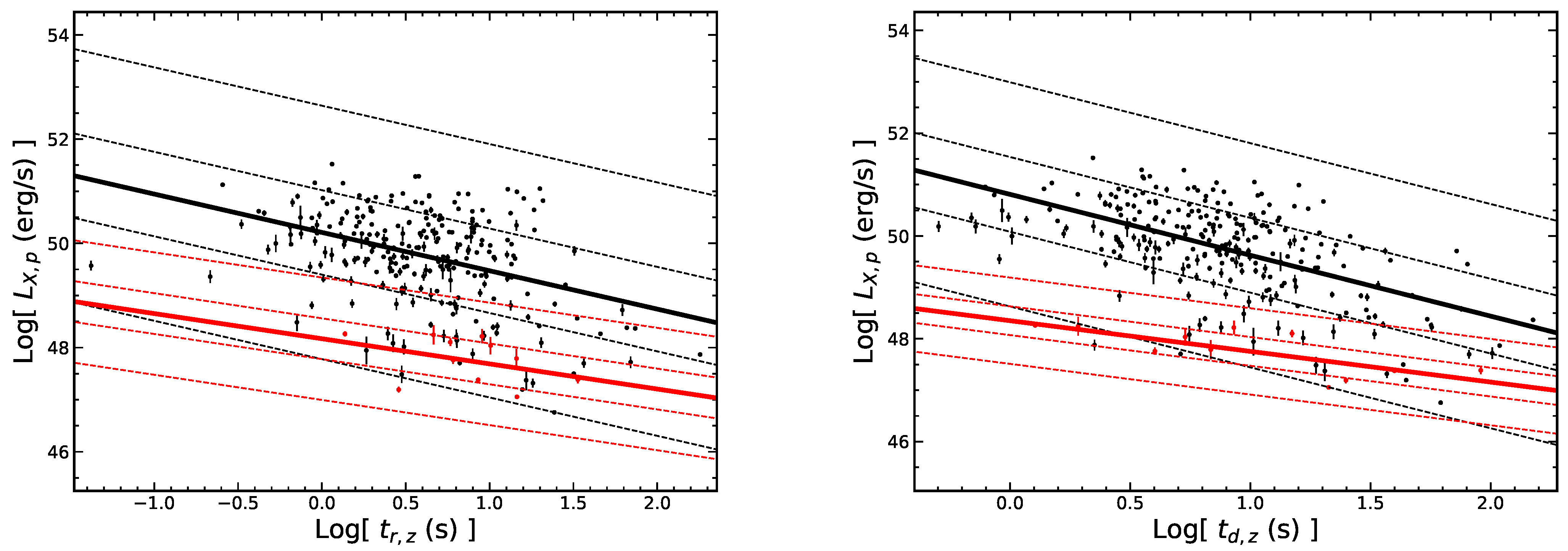
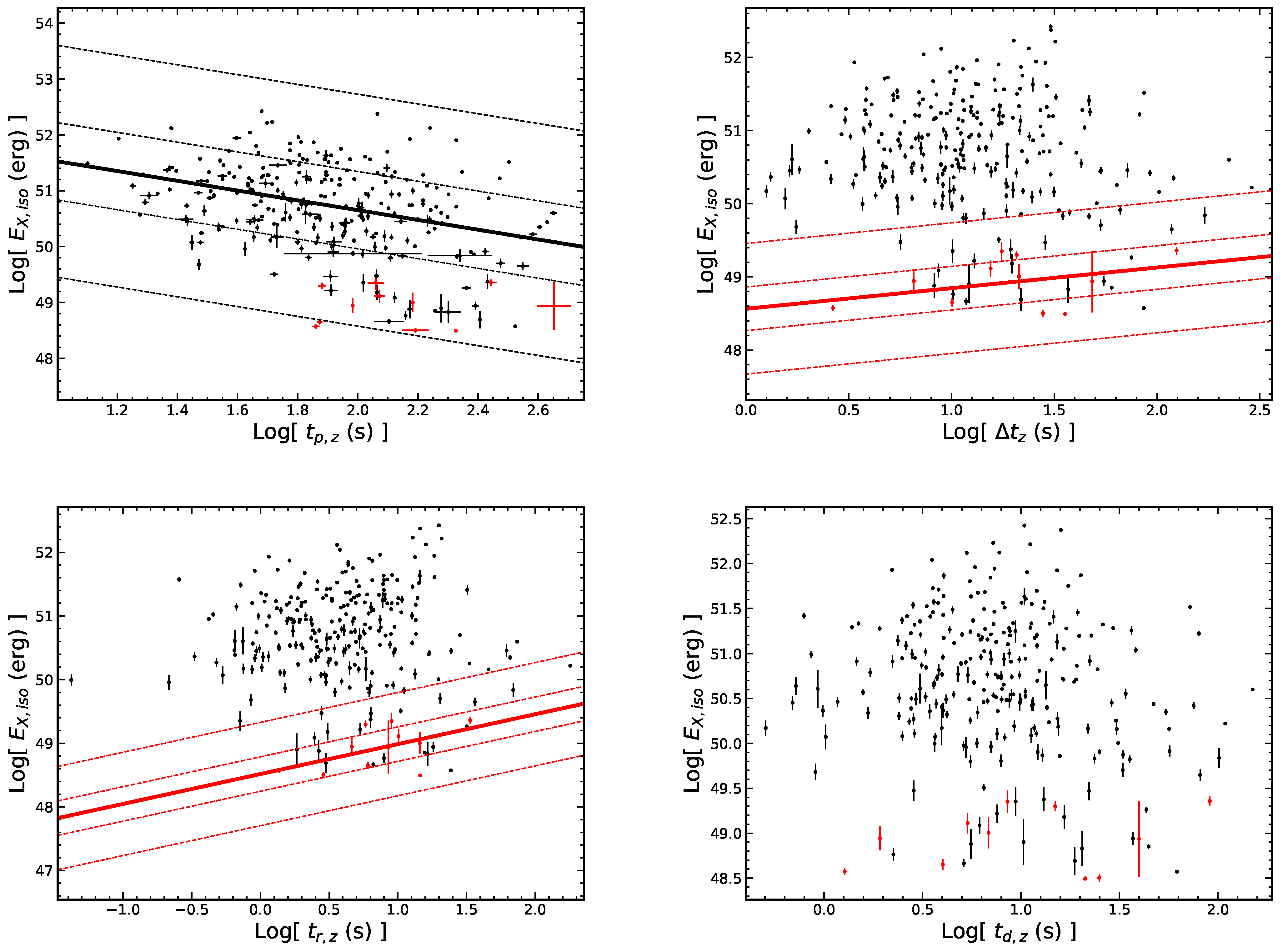
3.2. Two-Parameter Correlations of Early Flares and Late Flares
3.3. Two-Parameter Correlations of LGRB Flares and SGRB Flares
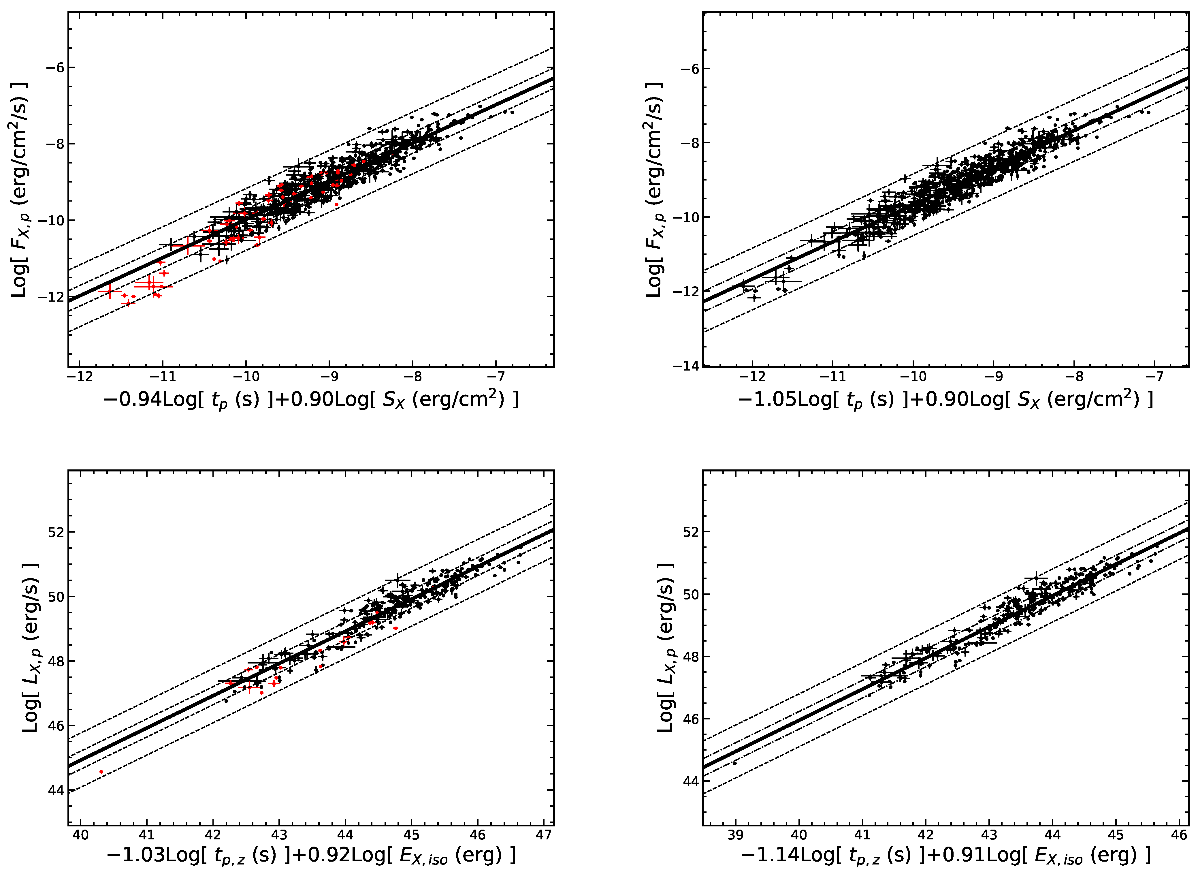
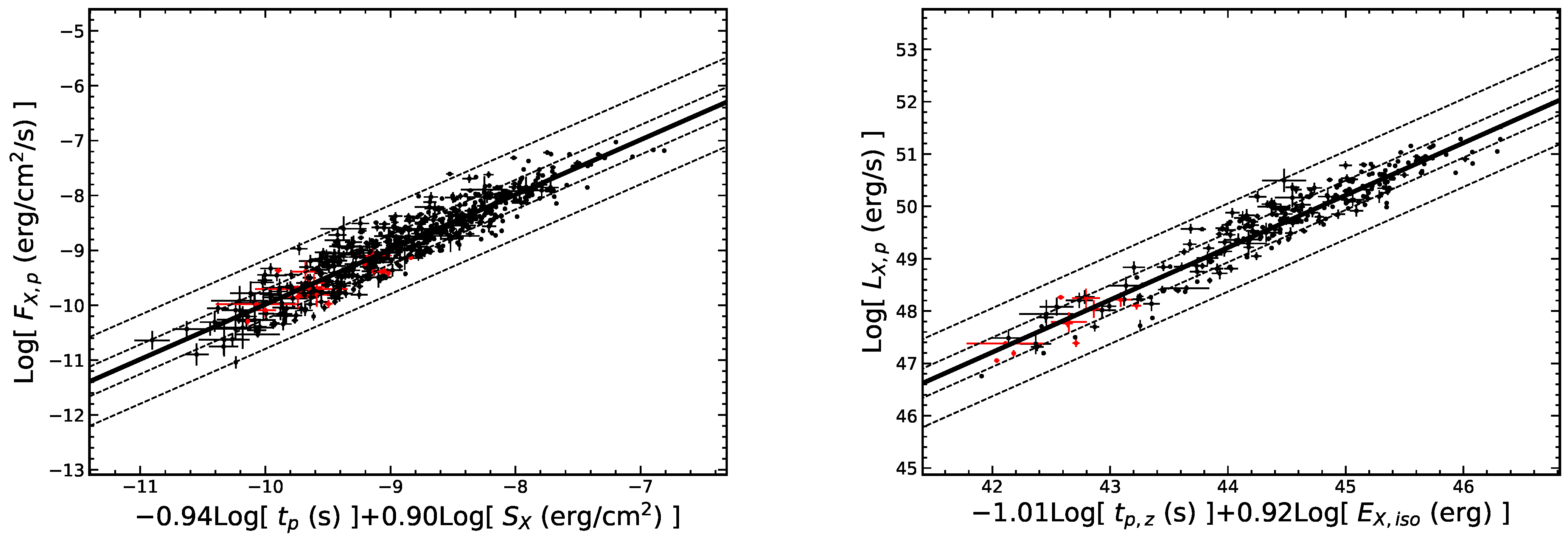
3.4. Three-Parameter Correlations of Flares
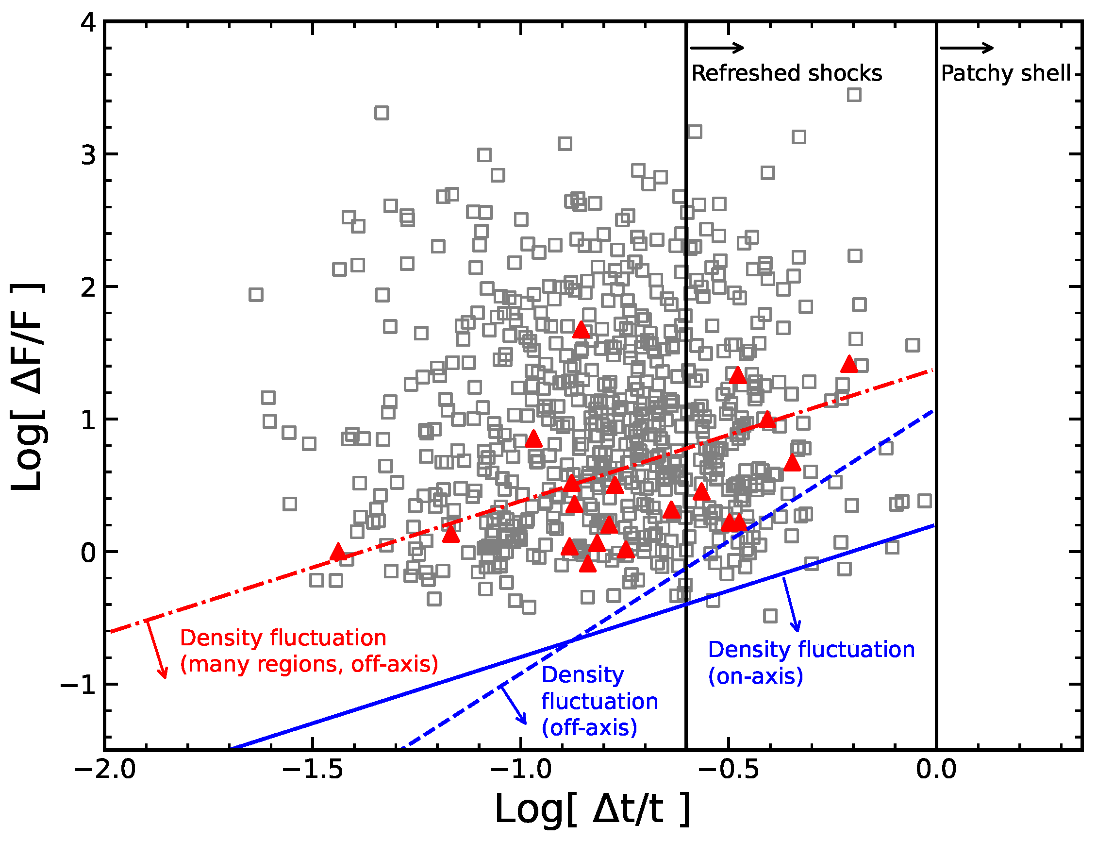
4. Origin of the Flares
5. Conclusions
Author Contributions
Funding
Data Availability Statement
Acknowledgments
Conflicts of Interest
References
- Kouveliotou, C.; Meegan, C.A.; Fishman, G.J.; Bhat, N.P.; Briggs, M.S.; Koshut, T.M.; Paciesas, W.S.; Pendleton, G.N. Identification of Two Classes of Gamma-ray Bursts. Astrophys. J. 1993, 413, L101. [Google Scholar] [CrossRef]
- Zhang, Z.-B.; Choi, C.-S. An Analysis of the Durations of Swift Gamma-ray Bursts. Astron. Astrophys. 2008, 484, 293. [Google Scholar] [CrossRef]
- MacFadyen, A.I.; Woosley, S.E. Collapsars: Gamma-ray Bursts and Explosions in ”Failed Supernovae”. Astrophys. J. 1998, 524, 262. [Google Scholar] [CrossRef]
- Xu, D.; de Ugarte Postigo, A.; Leloudas, G.; Krühler, T.; Cano, Z.; Hjorth, J.; Malesani, D.; Fynbo, J.P.U.; Thöne, C.C.; Sánchez-Ramírez, R.; et al. Discovery of the Broad-lined Type Ic SN 2013cq Associated with the Very Energetic GRB 130427A. Astrophys. J. 2013, 776, 98. [Google Scholar] [CrossRef]
- Berger, E. The Environments of Short-duration Gamma-ray Bursts and Implications for Their Progenitors. New Astron. Rev. 2011, 55, 1. [Google Scholar] [CrossRef]
- Gehrels, N.; Ramirez-Ruiz, E.; Fox, D.B. Gamma-ray Bursts in the Swift Era. Annu. Rev. Astron. Astrophys. 2009, 47, 567. [Google Scholar] [CrossRef]
- Nakar, E. Short-hard Gamma-ray Bursts. Phys. Rep. 2007, 442, 166. [Google Scholar] [CrossRef]
- Burrows, D.N.; Romano, P.; Falcone, A.; Kobayashi, S.; Zhang, B.; Moretti, A.; O’Brien, P.T.; Goad, M.R.; Campana, S.; Page, K.L.; et al. Bright X-ray Flares in Gamma-ray Burst Afterglows. Science 2005, 309, 1833. [Google Scholar] [CrossRef]
- Butler, N.R.; Kocevski, D.; Bloom, J.S.; Curtis, J.L. A Complete Catalog of Swift Gamma-ray Burst Spectra and Durations: Demise of a Physical Origin for Pre-Swift High-Energy Correlations. Astrophys. J. 2007, 671, 656. [Google Scholar] [CrossRef]
- Evans, P.A.; Beardmore, A.P.; Page, K.L.; Osborne, J.P.; O’Brien, P.T.; Willingale, R.; Starling, R.L.C.; Burrows, D.N.; Godet, O.; Vetere, L.; et al. Methods and Results of an Automatic Analysis of a Complete Sample of Swift-XRT Observations of GRBs. Mon. Not. R. Astron. Soc. 2009, 397, 1177. [Google Scholar] [CrossRef]
- Falcone, A.D.; Burrows, D.N.; Lazzati, D.; Campana, S.; Kobayashi, S.; Zhang, B.; Mészáros, P.; Page, K.L.; Kennea, J.A.; Romano, P.; et al. The Giant X-ray Flare of GRB 050502B: Evidence for Late-Time Internal Engine Activity. Astrophys. J. 2006, 641, 1010. [Google Scholar] [CrossRef]
- Falcone, A.D.; Morris, D.; Racusin, J.; Chincarini, G.; Moretti, A.; Romano, P.; Burrows, D.N.; Pagani, C.; Stroh, M.; Grupe, D.; et al. The First Survey of X-ray Flares from Gamma-ray Bursts Observed by Swift: Spectral Properties and Energetics. Astrophys. J. 2007, 671, 1921. [Google Scholar] [CrossRef]
- O’Brien, P.T.; Willingale, R.; Osborne, J.; Goad, M.R.; Page, K.L.; Vaughan, S.; Rol, E.; Beardmore, A.; Godet, O.; Hurkett, C.P.; et al. The Early X-ray Emission from GRBs. Astrophys. J. 2006, 647, 1213. [Google Scholar] [CrossRef]
- D’Avanzo, P. Short Gamma-ray Bursts: A Review. J. High Energy Astrophys. 2015, 7, 73. [Google Scholar] [CrossRef]
- Li, L.; Liang, E.-W.; Tang, Q.-W.; Chen, J.-M.; Xi, S.-Q.; Lü, H.-J.; Gao, H.; Zhang, B.; Zhang, J.; Yi, S.-X.; et al. A Comprehensive Study of Gamma-ray Burst Optical Emission. I. Flares and Early Shallow-decay Component. Astrophys. J. 2012, 758, 27. [Google Scholar] [CrossRef]
- Margutti, R.; Bernardini, G.; Barniol Duran, R.; Guidorzi, C.; Shen, R.F.; Chincarini, G. On the Average Gamma-ray Burst X-ray Flaring Activity. Mon. Not. R. Astron. Soc. 2011, 410, 1064. [Google Scholar] [CrossRef]
- Nousek, J.A.; Kouveliotou, C.; Grupe, D.; Page, K.L.; Granot, J.; Ramirez-Ruiz, E.; Patel, S.K.; Burrows, D.N.; Mangano, V.; Barthelmy, S.; et al. Evidence for a Canonical Gamma-ray Burst Afterglow Light Curve in the Swift XRT Data. Astrophys. J. 2006, 642, 389. [Google Scholar] [CrossRef]
- Ruffini, R.; Wang, Y.; Aimuratov, Y.; Barres de Almeida, U.; Becerra, L.; Bianco, C.L.; Chen, Y.C.; Karlica, M.; Kovacevic, M.; Li, L.; et al. Early X-ray Flares in GRBs. Astrophys. J. 2018, 852, 53. [Google Scholar] [CrossRef]
- Zhang, B.; Fan, Y.Z.; Dyks, J.; Kobayashi, S.; Mészáros, P.; Burrows, D.N.; Nousek, J.A.; Gehrels, N. Physical Processes Shaping Gamma-ray Burst X-ray Afterglow Light Curves: Theoretical Implications from the Swift X-ray Telescope Observations. Astrophys. J. 2006, 642, 354. [Google Scholar] [CrossRef]
- Wang, F.Y.; Dai, Z.G. Self-organized Criticality in X-ray Flares of Gamma-ray-Burst Afterglows. Nat. Phys. 2013, 9, 465. [Google Scholar] [CrossRef]
- Curran, P.A.; Starling, R.L.C.; O’Brien, P.T.; Godet, O.; van der Horst, A.J.; Wijers, R.A.M.J. On the nature of late X-ray flares in Swift gamma-ray bursts. Astron. Astrophys. 2008, 487, 533. [Google Scholar] [CrossRef]
- Campana, S.; Tagliaferri, G.; Lazzati, D.; Chincarini, G.; Covino, S.; Page, K.; Romano, P.; Moretti, A.; Cusumano, G.; Mangano, V.; et al. The X-ray Afterglow of the Short Gamma Ray Burst 050724. Astron. Astrophys. 2006, 454, 113. [Google Scholar] [CrossRef][Green Version]
- Margutti, R.; Chincarini, G.; Granot, J.; Guidorzi, C.; Berger, E.; Bernardini, M.G.; Gehrels, N.; Soderberg, A.M.; Stamatikos, M.; Zaninoni, E. X-ray Flare Candidates in Short Gamma-ray Bursts. Mon. Not. R. Astron. Soc. 2011, 417, 2144. [Google Scholar] [CrossRef][Green Version]
- Wang, Y.; Aimuratov, Y.; Moradi, R.; Peresano, M.; Ruffini, R.; Shakeri, S. Revisiting the Statistics of X-ray Flares in Gamma-ray Bursts. Mem. Soc. Astron. Ital. 2018, 89, 293. [Google Scholar] [CrossRef]
- Chincarini, G.; Moretti, A.; Romano, P.; Falcone, A.D.; Morris, D.; Racusin, J.; Campana, S.; Covino, S.; Guidorzi, C.; Tagliaferri, G.; et al. The First Survey of X-ray Flares from Gamma-ray Bursts Observed by Swift: Temporal Properties and Morphology. Astrophys. J. 2007, 671, 1903. [Google Scholar] [CrossRef]
- Chincarini, G.; Mao, J.; Margutti, R.; Bernardini, M.G.; Guidorzi, C.; Pasotti, F.; Giannios, D.; Della Valle, M.; Moretti, A.; Romano, P.; et al. Unveiling the Origin of X-ray Flares in Gamma-ray Bursts. Mon. Not. R. Astron. Soc. 2010, 406, 2113. [Google Scholar] [CrossRef]
- Liang, E.W.; Zhang, B.; O’Brien, P.T.; Willingale, R.; Angelini, L.; Burrows, D.N.; Campana, S.; Chincarini, G.; Falcone, A.; Gehrels, N.; et al. Testing the Curvature Effect and Internal Origin of Gamma-ray Burst Prompt Emissions and X-ray Flares with Swift Data. Astrophys. J. 2006, 646, 351. [Google Scholar] [CrossRef]
- Liu, C.; Mao, J. GRB X-ray Flare Properties among Different GRB Subclasses. Astrophys. J. 2019, 884, 59. [Google Scholar] [CrossRef]
- Yi, S.-X.; Du, M.; Liu, T. Statistical Analyses of the Energies of X-ray Plateaus and Flares in Gamma-ray Bursts. Astrophys. J. 2022, 924, 69. [Google Scholar] [CrossRef]
- Chang, X.Z.; Peng, Z.Y.; Chen, J.M.; Yin, Y.; Wang, D.Z.; Wu, H. A Comprehensive Study of Multiflare GRB Spectral Lag. Astrophys. J. 2021, 922, 34. [Google Scholar] [CrossRef]
- Yi, S.-X.; Xie, W.; Ma, S.-B.; Lei, W.-H.; Du, M. Constraining Properties of GRB Central Engines with X-ray Flares. Mon. Not. R. Astron. Soc. 2021, 507, 1047. [Google Scholar] [CrossRef]
- Ioka, K.; Kobayashi, S.; Zhang, B. Variabilities of Gamma-ray Burst Afterglows: Long-acting Engine, Anisotropic Jet, or Many Fluctuating Regions? Astrophys. J. 2005, 631, 429. [Google Scholar] [CrossRef]
- Mu, H.-J.; Gu, W.; Hou, S.-J.; Liu, T.; Lin, D.-B.; Yi, T.; Liang, E.-W.; Lu, J.-F. Central Engine of Late-time X-ray Flares with Internal Origin. Astrophys. J. 2016, 832, 161. [Google Scholar] [CrossRef]
- King, A.; O’Brien, P.T.; Goad, M.R.; Osborne, J.; Olsson, E.; Page, K. Gamma-ray Bursts: Restarting the Engine. Astrophys. J. 2005, 630, L113. [Google Scholar] [CrossRef][Green Version]
- Perna, R.; Armitage, P.J.; Zhang, B. Flares in Long and Short Gamma-ray Bursts: A Common Origin in a Hyperaccreting Accretion Disk. Astrophys. J. 2006, 636, L29. [Google Scholar] [CrossRef]
- Yi, S.-X.; Xi, S.-Q.; Yu, H.; Wang, F.Y.; Mu, H.-J.; Lü, L.Z.; Liang, E.-W. Comprehensive Study of the X-ray Flares from Gamma-ray Bursts Observed by Swift. Astrophys. J. Suppl. Ser. 2016, 224, 20. [Google Scholar] [CrossRef]
- Duque, R.; Beniamini, P.; Daigne, F.; Mochkovitch, R. Flares in Gamma-ray Burst X-ray Afterglows as Prompt Emission from Slightly Misaligned Structured Jets. Mon. Not. R. Astron. Soc. 2022, 513, 951. [Google Scholar] [CrossRef]
- Fan, Y.Z.; Wei, D.M. Late Internal-shock Model for Bright X-ray Flares in Gamma-ray Burst Afterglows and GRB 011121. Mon. Not. R. Astron. Soc. Lett. 2005, 364, L42. [Google Scholar] [CrossRef]
- Romano, P.; Moretti, A.; Banat, P.L.; Burrows, D.N.; Campana, S.; Chincarini, G.; Covino, S.; Malesani, D.; Tagliaferri, G.; Kobayashi, S.; et al. X-ray Flare in XRF 050406: Evidence for Prolonged Engine Activity. Astron. Astrophys. 2006, 836, 570. [Google Scholar] [CrossRef]
- Zhao, L.; Gao, H.; Lei, W.; Lan, L.; Liu, L. Giant X-ray and Optical Bump in GRBs: Evidence for Fallback Accretion Model. Astrophys. J. 2021, 906, 60. [Google Scholar] [CrossRef]
- Zheng, T.-C.; Li, L.; Zou, L.; Wang, X.-G. X-ray Flares Raising upon Magnetar Plateau as an Implication of a Surrounding Disk of Newborn Magnetized Neutron Star. Res. Astron. Astrophys. 2021, 21, 300. [Google Scholar] [CrossRef]
- Evans, P.A.; Beardmore, A.P.; Page, K.L.; Tyler, L.G.; Osborne, J.P.; Goad, M.R.; O’Brien, P.T.; Vetere, L.; Racusin, J.; Morris, D.; et al. An online repository of Swift/XRT light curves of γ-ray bursts. Astron. Astrophys. 2007, 469, 379. [Google Scholar] [CrossRef]
- Liang, E.-W.; Zhang, B.-B.; Zhang, B. A Comprehensive Analysis of Swift XRT Data. II. Diverse Physical Origins of the Shallow Decay Segment. Astrophys. J. 2007, 670, 565. [Google Scholar] [CrossRef]
- Wang, X.G.; Zhang, B.; Liang, E.W.; Lu, R.J.; Lin, D.B.; Li, J.; Li, L. Gamma-ray burst jet breaks revisited. Astrophys. J. 2018, 859, 160. [Google Scholar] [CrossRef]
- Bernardini, M.G.; Margutti, R.; Chincarini, G.; Guidorzi, C.; Mao, J. Gamma-ray Burst Long Lasting X-ray Flaring Activity. Astron. Astrophys. 2011, 526, A27. [Google Scholar] [CrossRef]
- Liang, E.; Zhang, B. Model-independent Multivariable Gamma-ray Burst Luminosity Indicator and Its Possible Cosmological Implications. Astrophys. J. 2005, 633, 611. [Google Scholar] [CrossRef]
- Dainotti, M.G.; Del Vecchio, R.; Tarnopolski, M. Gamma-ray Burst Prompt Correlations. Adv. Astron. 2018, 2018, 4969503. [Google Scholar] [CrossRef]
- Schaefer, B.E. The Hubble Diagram to Redshift >6 from 69 Gamma-ray Bursts. Astrophys. J. 2007, 660, 16. [Google Scholar] [CrossRef]
- Zhang, Z.B.; Zhang, C.T.; Zhao, Y.X.; Luo, J.J.; Jiang, L.Y.; Wang, X.L.; Han, X.L.; Terheide, R.K. Spectrum-energy Correlations in GRBs: Update, Reliability, and the Long/Short Dichotomy. Publ. Astron. Soc. Pac. 2018, 130, 054202. [Google Scholar] [CrossRef]
- Swenson, C.A.; Roming, P.W.A. Gamma-ray Burst Flares: X-ray Flaring. II. Astrophys. J. 2014, 788, 30. [Google Scholar] [CrossRef]


| GRB | Type a | z b | Flare | c | c | ||||||||||
|---|---|---|---|---|---|---|---|---|---|---|---|---|---|---|---|
| (Index) | (s) | (erg/cm2/s) | (erg/cm2) | (s) | (s) | (s) | |||||||||
| 050406 | Long | (1) | 3 | −3.22 ± 0.53 | 7.12 ± 0.57 | 213.17 ± 7.44 | 13.82 ± 1.49 | 0.88 ± 0.08 | 82.54 | 149.71 | 47.81 | 34.73 | 0.39 | 0.73 | |
| 050502B | Long | 5.2 ph | (1) | 1 | −9.54 ± 0.09 | 10.59 ± 0.09 | 720.54 ± 0.65 | 328.51 ± 3.47 | 49.36 ± 0.5 | 188.97 | 200.79 | 90.24 | 98.72 | 0.26 | 1.09 |
| (2) | 3 | −10.04 ± 0 | 1.84 ± 0.28 | 29,898.12 ± 161.76 | 0.07 ± 0.02 | 0.92 ± 0.2 | 18,695.09 | 2.23 | 3624.95 | 15,070.15 | 0.63 | 4.16 | |||
| (3) | 3 | −2.87 ± 0.33 | 5.09 ± 0.27 | 76,142.81 ± 553.83 | 0.1 ± 0.01 | 2.85 ± 0.22 | 36,398.71 | 9.31 | 19,346.01 | 17,052.7 | 0.48 | 0.88 | |||
| 050607 | Long | (1) | 3 | −33.87 ± 15.17 | 7.93 ± 0.59 | 305.98 ± 3.5 | 91.75 ± 12.44 | 2.91 ± 0.28 | 41.84 | 17.05 | 10.93 | 30.9 | 0.14 | 2.83 | |
| 050712 | Long | (1) | 3 | −35.1 ± 14.18 | 50.34 ± 24.66 | 215.84 ± 2.38 | 35.04 ± 8.35 | 0.26 ± 0.05 | 9.55 | 1.66 | 5.28 | 4.27 | 0.04 | 0.81 | |
| (2) | 3 | −11.18 ± 3.14 | 32.48 ± 9.02 | 264.52 ± 3.44 | 38.15 ± 6.31 | 0.81 ± 0.1 | 27.51 | 1.75 | 18.08 | 9.43 | 0.1 | 0.52 | |||
| (3) | 3 | −141.29 ± 83.12 | 14.38 ± 1.67 | 474.14 ± 2.28 | 36 ± 6.66 | 0.79 ± 0.11 | 29.41 | 8.36 | 4.88 | 24.53 | 0.06 | 5.03 | |||
| (4) | 3 | −16.49 ± 8.67 | 3.74 ± 1.43 | 950.68 ± 44.11 | 4.04 ± 1.02 | 0.86 ± 0.16 | 283.34 | 4.16 | 68.9 | 214.44 | 0.3 | 3.11 | |||
| 050713A | Long | (1) | 3 | −29.48 ± 2.96 | 8.73 ± 0.31 | 109.7 ± 0.47 | 906.43 ± 45.91 | 10.02 ± 0.41 | 14.53 | 16.8 | 4.28 | 10.25 | 0.13 | 2.39 | |
| (2) | 3 | −41.67 ± 10.13 | 8.19 ± 0.52 | 167.79 ± 1.08 | 122.83 ± 10.61 | 1.97 ± 0.13 | 21.22 | 8.75 | 5.07 | 16.15 | 0.13 | 3.19 | |||
| 050714B | Long | 2.4383 | (1) | 3 | −9.31 ± 1.52 | 9.33 ± 1.13 | 386.3 ± 7.86 | 17.9 ± 1.67 | 1.06 ± 0.1 | 76.63 | 56.37 | 36.44 | 40.18 | 0.2 | 1.1 |
| 050716 | Long | (1) | 3 | −35.09 ± 20.09 | 16.07 ± 5.54 | 171.63 ± 3.27 | 44.48 ± 11.52 | 0.48 ± 0.1 | 14.14 | 0.52 | 5.17 | 8.97 | 0.08 | 1.74 | |
| (2) | 3 | −24.48 ± 9.69 | 9.07 ± 1.56 | 381.51 ± 6.61 | 20.45 ± 3.36 | 0.81 ± 0.1 | 52.15 | 1.1 | 17.07 | 35.08 | 0.14 | 2.06 | |||
| 050724 | Short | 0.258 | (1) | 3 | −14.11 ± 0.96 | 9.01 ± 0.56 | 266.6 ± 1.53 | 56.47 ± 3.6 | 1.95 ± 0.12 | 44.93 | 3.18 | 18.3 | 26.63 | 0.17 | 1.45 |
| (2) | 3 | −2.06 ± 0.26 | 4.2 ± 0.33 | 56,763.79 ± 586.8 | 0.18 ± 0.02 | 4.96 ± 0.4 | 35,000.6 | 26.19 | 18,734.69 | 16,265.92 | 0.62 | 0.87 | |||
| 050726 | Long | (1) | 3 | −59.05 ± 5.9 | 22.79 ± 14.05 | 162.86 ± 5.07 | 16.53 ± 8.2 | 0.11 ± 0.05 | 8.87 | 0.66 | 3.04 | 5.83 | 0.05 | 1.92 | |
| (2) | 3 | −14.98 ± 3.75 | 9.05 ± 1.61 | 266.51 ± 5.39 | 28.06 ± 3.37 | 0.94 ± 0.1 | 43.72 | 1.72 | 17.45 | 26.27 | 0.16 | 1.51 | |||
| 050730 | Long | 3.967 | (1) | 3 | −55.16 ± 22.44 | 22.76 ± 5.36 | 229.9 ± 2.06 | 70.44 ± 13.25 | 0.69 ± 0.1 | 12.83 | 1.05 | 4.52 | 8.31 | 0.06 | 1.84 |
| (2) | 3 | −14 ± 1.34 | 11.49 ± 0.84 | 432.33 ± 3.5 | 105.11 ± 4.98 | 5.15 ± 0.23 | 63.46 | 2.25 | 28.55 | 34.91 | 0.15 | 1.22 | |||
| (3) | 3 | −43.31 ± 10.05 | 11.14 ± 1.67 | 681.61 ± 4.54 | 53.07 ± 5.84 | 2.72 ± 0.22 | 67.49 | 1.36 | 18.76 | 48.73 | 0.1 | 2.6 | |||
| 050802 | Long | (1) | 3 | −5.18 ± 2.23 | 5.49 ± 1.91 | 439.4 ± 35.28 | 8.29 ± 1.21 | 0.98 ± 0.14 | 152.33 | 0.77 | 71 | 81.32 | 0.35 | 1.15 | |
| 050803 | Long | 3.5 ph | (1) | 3 | −1.57 ± 0.71 | 29.37 ± 2.94 | 766.27 ± 44.39 | 4.54 ± 1.15 | 1.11 ± 0.25 | 322.93 | 1.84 | 278.53 | 44.4 | 0.42 | 0.16 |
| (2) | 3 | −9.61 ± 8.34 | 4.51 ± 3.65 | 1164.34 ± 126.09 | 3.41 ± 1.28 | 0.93 ± 0.26 | 355.09 | 1.55 | 122.39 | 232.7 | 0.3 | 1.9 | |||
| 050820A | Long | 2.612 | (1) | 3 | −69.29 ± 3.19 | 2.6 ± 0.35 | 233.79 ± 0.54 | 823.3 ± 30.28 | 46.89 ± 1.4 | 78.64 | 82.02 | 5.88 | 72.77 | 0.34 | 12.38 |
| 050822 | Long | 1.434 | (1) | 3 | −15.53 ± 3.62 | 7.03 ± 0.71 | 236.31 ± 3.82 | 69.93 ± 7.05 | 2.41 ± 0.2 | 44.95 | 5.47 | 15.81 | 29.15 | 0.19 | 1.84 |
| (2) | 3 | −22.55 ± 1.77 | 7.99 ± 0.22 | 444.17 ± 1.94 | 186.19 ± 7.31 | 9.69 ± 0.31 | 68.16 | 140.57 | 21.72 | 46.44 | 0.15 | 2.14 | |||
| 050904 | Long | 6.29 | (1) | 3 | −5.02 ± 0.33 | 19.75 ± 1.65 | 466.3 ± 2.92 | 93.42 ± 4.55 | 6.85 ± 0.26 | 95.66 | 3.18 | 66.16 | 29.5 | 0.21 | 0.45 |
| (2) | 3 | −16.71 ± 0.88 | 9.07 ± 1.02 | 6741.66 ± 14.77 | 6.68 ± 0.43 | 5.43 ± 0.31 | 1057.36 | 47.69 | 405.3 | 652.06 | 0.16 | 1.61 | |||
| (3) | 3 | −17.33 ± 2.41 | 4.13 ± 1.96 | 13,862.36 ± 135.09 | 3.29 ± 0.47 | 9.33 ± 0.91 | 3765.46 | 99.23 | 948.46 | 2817 | 0.27 | 2.97 | |||
| (4) | 3 | −8.02 ± 4.52 | 5.13 ± 1.16 | 21,456.72 ± 367.59 | 3.33 ± 0.59 | 16.47 ± 2.44 | 6427.98 | 241.17 | 2523.67 | 3904.31 | 0.3 | 1.55 | |||
| 050908 | Long | 3.344 | (1) | 3 | −145.83 ± 0.03 | 7.2 ± 0.8 | 387.55 ± 0.89 | 19.9 ± 2.9 | 0.65 ± 0.09 | 44.55 | 26 | 4.44 | 40.12 | 0.11 | 9.04 |
| 050915A | Long | 2.5273 | (1) | 3 | −10 ± 3.74 | 7.64 ± 1.03 | 105.65 ± 3.04 | 45.58 ± 4.72 | 0.8 ± 0.07 | 22.69 | 9.27 | 9.76 | 12.93 | 0.21 | 1.32 |
| (2) | 3 | −63.47 ± 0.23 | 21.52 ± 2.15 | 525.43 ± 10.49 | 2.29 ± 0.89 | 0.05 ± 0.02 | 29.02 | 1.53 | 9.36 | 19.66 | 0.06 | 2.1 | |||
| 050916 | Long | (1) | 3 | −32.72 ± 3 | 14.68 ± 2.28 | 19,599.25 ± 221.17 | 5.32 ± 1.59 | 7.17 ± 2.04 | 1756.27 | 84.34 | 634.73 | 1121.54 | 0.09 | 1.77 | |
| 050922B | Long | 4.5ph | (1) | 3 | −14.84 ± 3.63 | 5.12 ± 0.3 | 373.13 ± 3.4 | 134.85 ± 6.44 | 9.23 ± 0.25 | 89.88 | 478.38 | 27.52 | 62.37 | 0.24 | 2.27 |
| (2) | 3 | −289.66 ± 203.11 | 23.24 ± 5.38 | 498.23 ± 1.74 | 35.77 ± 7.44 | 0.49 ± 0.07 | 18.28 | 134.91 | 2.63 | 15.65 | 0.04 | 5.96 | |||
| (3) | 3 | −9.94 ± 0.7 | 9.38 ± 0.34 | 820.11 ± 6.39 | 179.71 ± 8 | 21.85 ± 0.96 | 157.32 | 752.98 | 73.41 | 83.91 | 0.19 | 1.14 | |||
| 051117A | Long | (1) | 3 | −1.69 ± 0.46 | 5.64 ± 0.84 | 155.92 ± 7.16 | 207.49 ± 19.26 | 15.1 ± 0.95 | 93.64 | 0.74 | 57.64 | 35.99 | 0.6 | 0.62 | |
| (2) | 3 | −50.98 ± 27.47 | 5.57 ± 2.69 | 324.4 ± 5.16 | 64.72 ± 14.11 | 2.62 ± 0.4 | 54.34 | 0.47 | 9.04 | 45.29 | 0.17 | 5.01 | |||
| (3) | 3 | −3.84 ± 0.77 | 7.02 ± 1.15 | 447.8 ± 12.95 | 99.73 ± 13.23 | 12.27 ± 1.42 | 158.91 | 0.98 | 87.81 | 71.09 | 0.35 | 0.81 | |||
| (4) | 3 | −34.92 ± 11.19 | 17.2 ± 3.23 | 609.19 ± 5.51 | 53.18 ± 6.54 | 1.97 ± 0.19 | 48.15 | 0.7 | 18.16 | 29.99 | 0.08 | 1.65 | |||
| (5) | 3 | −20.35 ± 2.28 | 12.37 ± 3.57 | 945.34 ± 9.39 | 77.14 ± 6.72 | 6.73 ± 0.48 | 113.24 | 1.55 | 45.91 | 67.33 | 0.12 | 1.47 | |||
| (6) | 3 | −14.31 ± 3.92 | 30.73 ± 4.79 | 1109.67 ± 7.88 | 77.47 ± 8.24 | 6.04 ± 0.5 | 101.1 | 1.81 | 61.82 | 39.27 | 0.09 | 0.64 | |||
| (7) | 3 | −67.78 ± 4.95 | 7.92 ± 0.51 | 1318.83 ± 2.37 | 193.12 ± 6.91 | 22.3 ± 0.59 | 154.75 | 5.32 | 27.38 | 127.37 | 0.12 | 4.65 | |||
| (8) | 3 | −74.08 ± 35.22 | 12 ± 2.61 | 1543.3 ± 10.49 | 33.08 ± 6.11 | 3.14 ± 0.42 | 126.09 | 1.06 | 27.47 | 98.62 | 0.08 | 3.59 | |||
| 051210 | Short | (1) | 3 | −342.91 ± 0 | 5.36 ± 1.83 | 121.97 ± 0.36 | 21.52 ± 6.91 | 0.28 ± 0.09 | 17.69 | 0.81 | 0.73 | 16.97 | 0.15 | 23.4 | |
| 051227 | Short | (1) | 3 | −6.71 ± 5.02 | 3.78 ± 0.37 | 116.41 ± 6.84 | 38.16 ± 5.41 | 1.33 ± 0.14 | 45.63 | 9.97 | 16.55 | 29.08 | 0.39 | 1.76 | |
| 060105 | Long | (1) | 3 | −2.98 ± 0 | 1.99 ± 0.1 | 49,413.32 ± 198.46 | 0.11 ± 0.01 | 3.55 ± 0.25 | 40,832.9 | 2.39 | 14,031.99 | 26,800.91 | 0.83 | 1.91 | |
| 060111A | Long | 2.32 | (1) | 3 | −1.26 ± 0.36 | 6.75 ± 1.25 | 100.04 ± 4.04 | 226.25 ± 21.66 | 11.6 ± 0.71 | 65.94 | 25.4 | 44.84 | 21.1 | 0.66 | 0.47 |
| (2) | 3 | −8.28 ± 2.12 | 8.56 ± 1.02 | 167.37 ± 3.31 | 129.9 ± 7.05 | 3.69 ± 0.2 | 36.73 | 22.8 | 17.56 | 19.17 | 0.22 | 1.09 | |||
| (3) | 3 | −10.77 ± 0.44 | 5.93 ± 0.09 | 283.73 ± 1.09 | 463.53 ± 7.71 | 24.6 ± 0.35 | 69.13 | 128.62 | 25.97 | 43.16 | 0.24 | 1.66 | |||
| 060115 | Long | 3.53 | (1) | 3 | −8.67 ± 3.02 | 7.64 ± 1.29 | 409.45 ± 16 | 13.99 ± 2.15 | 1.01 ± 0.15 | 93.64 | 3.65 | 42.25 | 51.39 | 0.23 | 1.22 |
| 060124 | Long | 2.296 | (1) | 3 | −26.53 ± 4.56 | 2.46 ± 0.26 | 369.12 ± 4.03 | 80.69 ± 7.68 | 8.67 ± 0.68 | 146.32 | 9.18 | 20.15 | 126.16 | 0.4 | 6.26 |
| (2) | 3 | −8.11 ± 0.16 | 26.77 ± 0.87 | 573.87 ± 0.95 | 1743.87 ± 35.98 | 104.79 ± 1.78 | 78.31 | 227.65 | 52.71 | 25.6 | 0.14 | 0.49 | |||
| (3) | 3 | −36.29 ± 1.3 | 16.61 ± 0.31 | 700.38 ± 0.9 | 1477.89 ± 30.95 | 63.32 ± 1.13 | 55.79 | 205.24 | 20.4 | 35.39 | 0.08 | 1.73 | |||
| (4) | 3 | −308.02 ± 100.07 | 2.91 ± 1.61 | 977.62 ± 2.9 | 67.93 ± 5.05 | 13.19 ± 0.81 | 270.89 | 10.46 | 6.98 | 263.9 | 0.28 | 37.78 | |||
| 060202 | Long | 0.783 | (1) | 3 | −23.92 ± 5.95 | 4.89 ± 1.54 | 380.59 ± 5.91 | 66.48 ± 8.86 | 4.17 ± 0.38 | 83.24 | 1.02 | 19.65 | 63.59 | 0.22 | 3.24 |
| (2) | 3 | −14.66 ± 6.58 | 8.04 ± 4.19 | 532.62 ± 16.5 | 43.19 ± 9.78 | 3.15 ± 0.57 | 94.86 | 1.52 | 36.28 | 58.58 | 0.18 | 1.61 | |||
| (3) | 3 | −4.76 ± 1.23 | 8.03 ± 0.46 | 718.67 ± 12.47 | 83.92 ± 7.61 | 13.93 ± 1.08 | 214.45 | 5.97 | 117.31 | 97.14 | 0.3 | 0.83 | |||
| 060204B | Long | 2.3393 | (1) | 3 | −39.94 ± 6.82 | 11.91 ± 0.69 | 318.38 ± 1.39 | 94.31 ± 6.19 | 2.21 ± 0.11 | 30.76 | 10.72 | 9.21 | 21.55 | 0.1 | 2.34 |
| 060210 | Long | 3.91 | (1) | 3 | −77.05 ± 27.7 | 6.6 ± 0.49 | 106.04 ± 0.6 | 273.12 ± 21.78 | 2.89 ± 0.16 | 14.3 | 3.3 | 2.06 | 12.24 | 0.13 | 5.94 |
| (2) | 3 | −11.56 ± 0.75 | 9.4 ± 0.32 | 199.06 ± 1.12 | 315.17 ± 8.74 | 8.67 ± 0.23 | 35.62 | 6.43 | 15.83 | 19.79 | 0.18 | 1.25 | |||
| (3) | 3 | −48.11 ± 5.1 | 9.55 ± 0.37 | 371.81 ± 1.1 | 152.59 ± 7.18 | 4.64 ± 0.17 | 40.25 | 5.24 | 9.73 | 30.52 | 0.11 | 3.14 | |||
| 060223A | Long | 4.41 | (1) | 3 | −9.81 ± 2.33 | 5.22 ± 2.77 | 1509.55 ± 69.59 | 2.61 ± 0.55 | 0.83 ± 0.14 | 413.93 | 8.04 | 151.89 | 262.05 | 0.27 | 1.73 |
| 060312 | Long | (1) | 3 | −20.79 ± 10.77 | 19.2 ± 1.92 | 79.77 ± 2.27 | 51.76 ± 13.62 | 0.3 ± 0.08 | 7.39 | 1.28 | 3.51 | 3.87 | 0.09 | 1.1 | |
| (2) | 3 | −12.94 ± 4 | 17.65 ± 7.5 | 98.94 ± 2.05 | 212.22 ± 18.6 | 1.99 ± 0.14 | 12.11 | 9.25 | 6.47 | 5.63 | 0.12 | 0.87 | |||
| (3) | 3 | −86.56 ± 32.71 | 9.2 ± 0.43 | 109.71 ± 0.49 | 301.27 ± 39.48 | 2.43 ± 0.25 | 10.84 | 17.19 | 1.82 | 9.02 | 0.1 | 4.95 | |||
| (4) | 3 | −35.72 ± 1.58 | 2.89 ± 1.1 | 530.1 ± 9.81 | 1.76 ± 0.61 | 0.22 ± 0.07 | 171.83 | 3.11 | 22.21 | 149.62 | 0.32 | 6.74 | |||
| 060313 | Short | (1) | 3 | −6.44 ± 0.64 | 24.47 ± 2.45 | 100 ± 18.83 | 14.18 ± 6.73 | 0.18 ± 0.08 | 16.33 | 1.6 | 11.29 | 5.04 | 0.16 | 0.45 | |
| (2) | 3 | −29.09 ± 2.91 | 4.36 ± 4.02 | 131.91 ± 7.11 | 15.41 ± 7.8 | 0.35 ± 0.15 | 30.4 | 2.08 | 5.99 | 24.41 | 0.23 | 4.07 | |||
| (3) | 3 | −48.04 ± 4.8 | 7.42 ± 3.98 | 184.8 ± 184.58 | 19.67 ± 2.87 | 0.36 ± 0.04 | 24.51 | 3.3 | 5.1 | 19.42 | 0.13 | 3.81 | |||
| 060319 | Long | 1.172 | (1) | 3 | −54.43 ± 0.23 | 5.42 ± 1.56 | 251.57 ± 2.76 | 13.26 ± 4.35 | 0.42 ± 0.13 | 42.72 | 3.78 | 6.7 | 36.02 | 0.17 | 5.38 |
| 060413 | Long | (1) | 3 | −15.25 ± 4.54 | 4.99 ± 0.77 | 641.89 ± 15.83 | 46.11 ± 7.09 | 5.48 ± 0.67 | 156.44 | 8.86 | 46.61 | 109.83 | 0.24 | 2.36 | |
| (2) | 3 | −4.84 ± 3.33 | 9.21 ± 4.81 | 3181.75 ± 833.84 | 79.2 ± 12.57 | 54.26 ± 5.43 | 885.44 | 31.25 | 503.8 | 381.64 | 0.28 | 0.76 | |||
| 060418 | Long | 1.489 | (1) | 3 | −50.88 ± 3.15 | 8.83 ± 0.16 | 129.05 ± 0.3 | 2074.94 ± 74.98 | 22.92 ± 0.69 | 14.67 | 11.62 | 3.29 | 11.39 | 0.11 | 3.47 |
| 060510B | Long | 4.94 | (1) | 3 | −15.97 ± 3.55 | 22.87 ± 5.44 | 197.2 ± 2.66 | 124.74 ± 14.86 | 1.85 ± 0.2 | 19.14 | 0.43 | 10.45 | 8.69 | 0.1 | 0.83 |
| (2) | 3 | −24.41 ± 2.68 | 24.88 ± 2.52 | 300.06 ± 1.54 | 245.08 ± 12.77 | 4.26 ± 0.22 | 22.48 | 0.98 | 11.1 | 11.38 | 0.07 | 1.03 | |||
| 060512 | Long | 2.1 | (1) | 3 | −24.65 ± 9.11 | 7.61 ± 1.34 | 201.39 ± 3.54 | 35.98 ± 6.77 | 0.85 ± 0.13 | 31.09 | 3.66 | 9.29 | 21.81 | 0.15 | 2.35 |
| 060522 | Long | 5.11 | (1) | 3 | −6.22 ± 4.74 | 9.68 ± 2.02 | 163.79 ± 9.18 | 22.07 ± 4.27 | 0.67 ± 0.11 | 38.97 | 4.07 | 21.11 | 17.87 | 0.24 | 0.85 |
| 060526 | Long | 3.221 | (1) | 3 | −53.83 ± 2.51 | 13.16 ± 1.08 | 251.13 ± 0.48 | 1503.18 ± 66.48 | 23.61 ± 0.82 | 20.69 | 362.39 | 5.64 | 15.05 | 0.08 | 2.67 |
| (2) | 3 | −18.96 ± 3.01 | 9.76 ± 0.17 | 310.42 ± 1.52 | 628.07 ± 31.42 | 21.38 ± 0.88 | 44.29 | 203.56 | 16.68 | 27.61 | 0.14 | 1.65 | |||
| 060604 | Long | 2.1357 | (1) | 3 | −10.06 ± 0.82 | 6.19 ± 0.26 | 137.82 ± 1.07 | 371.83 ± 10.9 | 9.59 ± 0.24 | 33.54 | 250.4 | 13.18 | 20.37 | 0.24 | 1.55 |
| (2) | 3 | −114.53 ± 26.2 | 14.68 ± 1.21 | 169.35 ± 0.46 | 275.23 ± 21.04 | 2.21 ± 0.12 | 10.73 | 201.44 | 2.05 | 8.68 | 0.06 | 4.23 | |||
| 060607A | Long | 3.0749 | (1) | 3 | −2.91 ± 2.56 | 11.65 ± 7.57 | 82.4 ± 5.69 | 181.26 ± 48.67 | 3.94 ± 0.61 | 28.2 | 3.37 | 19.13 | 9.07 | 0.34 | 0.47 |
| (2) | 3 | −82.13 ± 27.05 | 5.52 ± 0.32 | 96.51 ± 0.5 | 449.97 ± 52.02 | 5.04 ± 0.48 | 15.19 | 8.99 | 1.84 | 13.35 | 0.16 | 7.23 | |||
| (3) | 3 | −15.64 ± 5.51 | 10.65 ± 4.34 | 178.65 ± 5.03 | 65.92 ± 9.38 | 1.33 ± 0.16 | 26.1 | 1.73 | 10.97 | 15.13 | 0.15 | 1.38 | |||
| (4) | 3 | −11.59 ± 1.01 | 7.99 ± 0.23 | 260.12 ± 1.6 | 353.97 ± 9.74 | 13.95 ± 0.34 | 51.12 | 11.01 | 21.28 | 29.84 | 0.2 | 1.4 | |||
| 060707 | Long | 3.425 | (1) | 3 | −402.95 ± 0 | 5.95 ± 1.36 | 186.74 ± 0.61 | 20.87 ± 5.68 | 0.37 ± 0.1 | 24.2 | 2.1 | 0.95 | 23.25 | 0.13 | 24.37 |
| 060714 | Long | 2.711 | (1) | 3 | −7.04 ± 5.2 | 62.09 ± 32.85 | 114.56 ± 1.76 | 246.48 ± 75.01 | 2.59 ± 0.57 | 13.94 | 37.27 | 11.27 | 2.67 | 0.12 | 0.24 |
| (2) | 3 | −5.46 ± 0.86 | 15.2 ± 1.52 | 138.66 ± 1.45 | 543.76 ± 30.62 | 12.35 ± 0.48 | 29.47 | 90.81 | 18.79 | 10.68 | 0.21 | 0.57 | |||
| (3) | 3 | −29.54 ± 3.78 | 13.77 ± 0.46 | 174.62 ± 0.63 | 409.66 ± 17.64 | 5.32 ± 0.18 | 16.93 | 77.13 | 6.2 | 10.72 | 0.1 | 1.73 | |||
| 060719 | Long | 1.532 | (1) | 3 | −14.76 ± 10.08 | 9.71 ± 3.05 | 206.46 ± 10.59 | 10.88 ± 2.89 | 0.27 ± 0.06 | 32.64 | 4.43 | 13.49 | 19.15 | 0.16 | 1.42 |
| 060729 | Long | 0.54 | (1) | 3 | −28.56 ± 3.55 | 6.72 ± 0.11 | 177.25 ± 0.71 | 1056.29 ± 40.86 | 23.02 ± 0.65 | 28.81 | 3.11 | 7.48 | 21.33 | 0.16 | 2.85 |
| 060804 | Long | (1) | 3 | −44.67 ± 4.47 | 7.17 ± 5.15 | 446.74 ± 234.41 | 5.48 ± 0.87 | 0.25 ± 0.03 | 61.88 | 1.01 | 13.14 | 48.75 | 0.14 | 3.71 | |
| 060814 | Long | 1.9229 | (1) | 3 | −44.3 ± 13.05 | 3.05 ± 0.06 | 129.77 ± 1.18 | 571.55 ± 29.52 | 16.27 ± 0.57 | 38.86 | 1.23 | 4.54 | 34.32 | 0.3 | 7.56 |
| 060904A | Long | (1) | 3 | −8.92 ± 0.85 | 10.51 ± 0.71 | 319.51 ± 3.46 | 54.64 ± 2.81 | 2.57 ± 0.13 | 60.81 | 6.01 | 30.57 | 30.24 | 0.19 | 0.99 | |
| (2) | 3 | −88.24 ± 29.57 | 9.5 ± 0.92 | 675.74 ± 3.97 | 15.49 ± 1.85 | 0.75 ± 0.07 | 64.75 | 5.19 | 10.98 | 53.77 | 0.1 | 4.9 | |||
| 060904B | Long | 0.703 | (1) | 3 | −27.14 ± 2.54 | 6.41 ± 0.64 | 155.26 ± 1.26 | 1060.64 ± 204.72 | 21.27 ± 3.8 | 26.52 | 95.25 | 6.88 | 19.64 | 0.17 | 2.85 |
| (2) | 3 | −22.7 ± 10.83 | 6.38 ± 2.41 | 176.03 ± 2.35 | 1434.06 ± 606.99 | 34.54 ± 12.48 | 31.73 | 140.46 | 8.97 | 22.76 | 0.18 | 2.54 | |||
| 060926 | Long | 3.2 | (1) | 3 | −32.82 ± 3.28 | 2.43 ± 0.82 | 404.61 ± 214.05 | 2.93 ± 0.36 | 0.34 ± 0.03 | 157.48 | 1.65 | 18.73 | 138.75 | 0.39 | 7.41 |
| 060929 | Long | (1) | 3 | −7.44 ± 0.42 | 9.66 ± 0.16 | 538.48 ± 2.49 | 236.03 ± 4.66 | 21.36 ± 0.39 | 116.97 | 669.98 | 60.23 | 56.75 | 0.22 | 0.94 | |
| 061121 | Long | 1.314 | (1) | 3 | −23.34 ± 3.73 | 38.7 ± 6.39 | 74.93 ± 0.47 | 6045.83 ± 610.34 | 21.81 ± 1.92 | 4.67 | 2.19 | 2.68 | 1.99 | 0.06 | 0.74 |
| (2) | 3 | −40.94 ± 16.38 | 14.54 ± 1.38 | 118.47 ± 1.06 | 381.19 ± 54.23 | 2.88 ± 0.31 | 9.88 | 0.91 | 3.23 | 6.65 | 0.08 | 2.06 | |||
| 061202 | Long | 2.2543 | (1) | 3 | −11.57 ± 1.69 | 5.09 ± 0.17 | 140.26 ± 1.3 | 391.52 ± 15.12 | 11.03 ± 0.31 | 36.84 | 1475.37 | 12.51 | 24.33 | 0.26 | 1.94 |
| (2) | 3 | −181.33 ± 0.04 | 2 ± 0.2 | 239.43 ± 3.68 | 16.22 ± 2.64 | 1.18 ± 0.19 | 102.52 | 48.73 | 2.83 | 99.69 | 0.43 | 35.19 | |||
| 070103 | Long | 2.6208 | (1) | 3 | −2.42 ± 1.56 | 2.42 ± 1.1 | 790.91 ± 193.46 | 0.91 ± 0.23 | 0.43 ± 0.11 | 618.61 | 1.08 | 251.1 | 367.51 | 0.78 | 1.46 |
| 070107 | Long | (1) | 3 | −90.28 ± 0.01 | 30.8 ± 0.04 | 321.39 ± 0.47 | 140.98 ± 10.34 | 1.34 ± 0.1 | 12.39 | 7.06 | 4.03 | 8.36 | 0.04 | 2.07 | |
| (2) | 3 | −26.1 ± 0.06 | 94.45 ± 0.02 | 359.29 ± 0.65 | 128.89 ± 11.27 | 1.48 ± 0.13 | 15.06 | 7.1 | 10.5 | 4.56 | 0.04 | 0.43 | |||
| (3) | 3 | −9.02 ± 0.48 | 10.57 ± 0.63 | 381.83 ± 1.07 | 136.8 ± 5.3 | 7.63 ± 0.28 | 72.07 | 7.94 | 36.18 | 35.88 | 0.19 | 0.99 | |||
| (4) | 3 | −28.94 ± 0.24 | 18.42 ± 0.66 | 445.29 ± 1.14 | 63.01 ± 6.57 | 1.77 ± 0.18 | 36.4 | 4.18 | 15.19 | 21.21 | 0.08 | 1.4 | |||
| (5) | 3 | −36.39 ± 0 | 15.64 ± 0 | 1354.07 ± 0 | 9.57 ± 1.46 | 0.82 ± 0.13 | 112.02 | 1.66 | 39.83 | 72.19 | 0.08 | 1.81 | |||
| (6) | 3 | −6.68 ± 1.82 | 4.52 ± 0.69 | 87,733.69 ± 1004.11 | 0.11 ± 0.01 | 2.52 ± 0.29 | 30,612.35 | 1.28 | 12,109.67 | 18,502.68 | 0.35 | 1.53 | |||
| 070129 | Long | 2.3384 | (1) | 3 | −18.47 ± 4.98 | 25.15 ± 18.5 | 210.54 ± 4.08 | 65.79 ± 10.12 | 0.92 ± 0.12 | 18.09 | 1.06 | 9.75 | 8.34 | 0.09 | 0.85 |
| (2) | 3 | −32.37 ± 20.42 | 9.64 ± 4.77 | 238.41 ± 3.99 | 77.99 ± 18.78 | 1.7 ± 0.27 | 28.57 | 1.79 | 8.48 | 20.09 | 0.12 | 2.37 | |||
| (3) | 3 | −21.29 ± 1.79 | 14.37 ± 3.59 | 307.47 ± 2.24 | 696.48 ± 47.19 | 17.77 ± 1.02 | 33.07 | 33.03 | 14.01 | 19.07 | 0.11 | 1.36 | |||
| (4) | 3 | −13.18 ± 2.35 | 32.39 ± 1.96 | 366.67 ± 1.6 | 1054.42 ± 56.21 | 27.94 ± 1.08 | 34.43 | 82.31 | 21.78 | 12.65 | 0.09 | 0.58 | |||
| (5) | 3 | −23.77 ± 2.2 | 9.94 ± 0.61 | 444.4 ± 1.71 | 374.91 ± 13.44 | 16.56 ± 0.44 | 57.66 | 50.09 | 19.96 | 37.69 | 0.13 | 1.89 | |||
| (6) | 3 | −37.3 ± 8.86 | 13.79 ± 4.97 | 550.52 ± 5.16 | 117.21 ± 16.18 | 4.4 ± 0.44 | 49.1 | 28.09 | 16.3 | 32.8 | 0.09 | 2.01 | |||
| (7) | 3 | −304.87 ± 0.22 | 12.67 ± 4.35 | 578.86 ± 0.95 | 88.52 ± 13.97 | 2.37 ± 0.34 | 36.49 | 24.25 | 3.28 | 33.21 | 0.06 | 10.12 | |||
| (8) | 3 | −52.78 ± 15.12 | 15.08 ± 1.36 | 664.24 ± 2.59 | 68.14 ± 7.12 | 2.59 ± 0.2 | 49.85 | 26.7 | 14.72 | 35.13 | 0.08 | 2.39 | |||
| (9) | 3 | −47.8 ± 2.98 | 16.8 ± 6.2 | 901.92 ± 12.48 | 3.69 ± 1.22 | 0.18 ± 0.06 | 64.75 | 2.99 | 21.12 | 43.63 | 0.07 | 2.07 | |||
| 070306 | Long | 1.4959 | (1) | 3 | −34.05 ± 6.43 | 7.77 ± 0.31 | 181.17 ± 0.98 | 299.03 ± 18.62 | 5.68 ± 0.26 | 25.12 | 1.1 | 6.47 | 18.65 | 0.14 | 2.88 |
| 070318 | Long | 0.836 | (1) | 3 | −7.35 ± 0.79 | 4.69 ± 0.27 | 284.45 ± 4.6 | 76.91 ± 3.76 | 5.52 ± 0.24 | 93.39 | 3.19 | 36.31 | 57.08 | 0.33 | 1.57 |
| 070330 | Long | (1) | 3 | −6.23 ± 1.24 | 4.03 ± 0.41 | 211.67 ± 8.84 | 22.01 ± 2.64 | 1.38 ± 0.15 | 81.76 | 136.61 | 31.43 | 50.33 | 0.39 | 1.6 | |
| 070419B | Long | 1.9591 | (1) | 3 | −11 ± 0.94 | 4.98 ± 0.2 | 231.86 ± 2.02 | 467.33 ± 16.94 | 22.5 ± 0.65 | 62.96 | 1.7 | 21.59 | 41.36 | 0.27 | 1.92 |
| 070518 | Long | (1) | 3 | −3.55 ± 0.8 | 13.47 ± 10.51 | 109.33 ± 2.9 | 71.87 ± 34.38 | 1.75 ± 0.71 | 31.57 | 50.62 | 21.36 | 10.21 | 0.29 | 0.48 | |
| (2) | 3 | −5.95 ± 0.59 | 4.34 ± 0.45 | 140.26 ± 6.18 | 43.51 ± 11.42 | 1.76 ± 0.45 | 52.58 | 37.29 | 21.26 | 31.32 | 0.37 | 1.47 | |||
| (3) | 3 | −15.93 ± 3.59 | 10.9 ± 1.02 | 188.05 ± 2.22 | 83.05 ± 5.91 | 1.72 ± 0.11 | 26.88 | 89.7 | 11.33 | 15.56 | 0.14 | 1.37 | |||
| 070520B | Long | (1) | 1 | −16.09 ± 0.93 | 6.07 ± 0.15 | 194.13 ± 1.5 | 229.68 ± 8.8 | 9.99 ± 0.22 | 55.26 | 5.81 | 20.36 | 34.89 | 0.28 | 1.71 | |
| 070621 | Long | (1) | 3 | −25.5 ± 6.97 | 19.89 ± 4.86 | 146.62 ± 1.84 | 103.89 ± 12.49 | 0.97 ± 0.11 | 12.12 | 1.08 | 5.45 | 6.67 | 0.08 | 1.22 | |
| (2) | 3 | −16.59 ± 8.35 | 7 ± 0.86 | 192.68 ± 4.4 | 33.96 ± 4.73 | 0.93 ± 0.1 | 35.92 | 1.27 | 12.26 | 23.66 | 0.19 | 1.93 | |||
| 070704 | Long | (1) | 1 | −25.76 ± 0.99 | 5.86 ± 0.11 | 316.34 ± 1.19 | 526.61 ± 16.53 | 31.58 ± 0.59 | 76.88 | 50.73 | 24.61 | 52.27 | 0.24 | 2.12 | |
| 070721B | Long | 3.626 | (1) | 3 | −126.52 ± 0.02 | 14.01 ± 7.56 | 266.19 ± 1.41 | 116.27 ± 48.21 | 1.49 ± 0.57 | 17.21 | 4.73 | 3.01 | 14.2 | 0.06 | 4.72 |
| (2) | 3 | −87.61 ± 65.34 | 63.68 ± 15.69 | 310.31 ± 3.83 | 248.15 ± 126.45 | 1.48 ± 0.72 | 7.74 | 9.6 | 3.45 | 4.29 | 0.02 | 1.25 | |||
| (3) | 3 | −58.49 ± 24.07 | 25.75 ± 4.72 | 346.32 ± 2.4 | 87.32 ± 14.32 | 1.17 ± 0.15 | 17.47 | 3.32 | 6.34 | 11.13 | 0.05 | 1.75 | |||
| 070724A | Short | 0.457 | (1) | 3 | −9.74 ± 2.66 | 20.37 ± 5.3 | 108.88 ± 2.18 | 75.11 ± 12.12 | 0.85 ± 0.11 | 14.66 | 2.29 | 8.83 | 5.83 | 0.13 | 0.66 |
| (2) | 3 | −7.8 ± 2.64 | 26.8 ± 1.33 | 221.85 ± 3.8 | 80.36 ± 34.19 | 1.91 ± 0.76 | 31.04 | 47.43 | 21.07 | 9.97 | 0.14 | 0.47 | |||
| 071021 | Long | 2.452 | (1) | 3 | −15.17 ± 2.59 | 16.94 ± 2.56 | 219.02 ± 2.8 | 169.92 ± 15.87 | 3.31 ± 0.3 | 25.21 | 2.38 | 12.69 | 12.52 | 0.12 | 0.99 |
| (2) | 3 | −12.66 ± 1.78 | 10.79 ± 0.98 | 6214.18 ± 20.07 | 2.84 ± 0.23 | 2.17 ± 0.17 | 988.68 | 18.14 | 449.34 | 539.34 | 0.16 | 1.2 | |||
| 071031 | Long | 2.692 | (1) | 3 | −1.18 ± 0.28 | 7.97 ± 1.05 | 145.78 ± 4.37 | 714.94 ± 52.02 | 52.78 ± 2.45 | 95.07 | 73.03 | 68.02 | 27.05 | 0.65 | 0.4 |
| (2) | 3 | −31.87 ± 9.32 | 6.19 ± 0.94 | 199.85 ± 1.7 | 240.85 ± 33.22 | 6.11 ± 0.64 | 33.71 | 34.66 | 7.88 | 25.83 | 0.17 | 3.28 | |||
| (3) | 3 | −30.51 ± 8.6 | 8.42 ± 0.94 | 258.62 ± 1.81 | 133.23 ± 14.84 | 3.52 ± 0.29 | 34.8 | 25.37 | 9.9 | 24.9 | 0.13 | 2.52 | |||
| (4) | 3 | −9.04 ± 0.94 | 3.74 ± 0.1 | 449.96 ± 4.06 | 93.98 ± 3.04 | 11.45 ± 0.28 | 159.89 | 32.67 | 51.31 | 108.58 | 0.36 | 2.12 | |||
| 071112C | Long | 0.823 | (1) | 3 | −10.27 ± 4.97 | 3.87 ± 0.64 | 645.79 ± 30.74 | 15.37 ± 2.95 | 2.51 ± 0.38 | 214.8 | 1.58 | 66.51 | 148.3 | 0.33 | 2.23 |
| 071118 | Long | (1) | 3 | −57.31 ± 5.73 | 4.95 ± 1.97 | 210.87 ± 5.12 | 18.86 ± 5.07 | 0.54 ± 0.13 | 38.52 | 0.59 | 5.48 | 33.04 | 0.18 | 6.02 | |
| (2) | 3 | −175.08 ± 0.02 | 2.66 ± 0.57 | 368.13 ± 1.47 | 17.48 ± 4.12 | 1.44 ± 0.33 | 114.85 | 1.94 | 4.29 | 110.56 | 0.31 | 25.75 | |||
| (3) | 3 | −12.99 ± 4.29 | 6.92 ± 1.14 | 603.09 ± 15.74 | 34.92 ± 4.56 | 3.32 ± 0.36 | 123.8 | 7.62 | 46.4 | 77.4 | 0.21 | 1.67 | |||
| 071122 | Long | 1.14 | (1) | 3 | −153.8 ± 0.03 | 13.61 ± 6.41 | 405.36 ± 2.42 | 12.05 ± 7.4 | 0.23 ± 0.14 | 26 | 2.45 | 3.94 | 22.06 | 0.06 | 5.6 |
| 080210 | Long | 2.641 | (1) | 3 | −22.5 ± 3.84 | 12.66 ± 1.36 | 191.03 ± 2.01 | 166.05 ± 16.98 | 2.77 ± 0.25 | 21.68 | 16.9 | 8.54 | 13.14 | 0.11 | 1.54 |
| 080212 | Long | (1) | 3 | −27.22 ± 4.76 | 6.38 ± 3.83 | 191.55 ± 3.34 | 107.3 ± 16.06 | 2.66 ± 0.25 | 32.82 | 5.25 | 8.48 | 24.34 | 0.17 | 2.87 | |
| (2) | 3 | −20.12 ± 3.63 | 6.58 ± 0.89 | 238.65 ± 1.79 | 360.86 ± 37.57 | 11.98 ± 0.99 | 43.61 | 46.89 | 13.26 | 30.36 | 0.18 | 2.29 | |||
| (3) | 3 | −11.46 ± 1.61 | 9.3 ± 0.76 | 296.61 ± 2.56 | 342.17 ± 18.01 | 14.16 ± 0.69 | 53.6 | 78.32 | 23.8 | 29.8 | 0.18 | 1.25 | |||
| 080310 | Long | 2.42 | (1) | 3 | −34.6 ± 5.5 | 2.92 ± 0.14 | 147.71 ± 1 | 253.85 ± 20.22 | 8.88 ± 0.6 | 47.59 | 6.52 | 6.33 | 41.25 | 0.32 | 6.51 |
| (2) | 3 | −29.51 ± 7.67 | 6.45 ± 4.1 | 193.05 ± 3.15 | 257.5 ± 53.52 | 6.25 ± 0.88 | 32.12 | 13.3 | 8.01 | 24.11 | 0.17 | 3.01 | |||
| (3) | 3 | −7.71 ± 2.46 | 6.98 ± 2.43 | 231.07 ± 8.27 | 282.41 ± 81.99 | 12.78 ± 3.64 | 58.56 | 22.88 | 26.51 | 32.05 | 0.25 | 1.21 | |||
| (4) | 3 | −101.83 ± 71.92 | 18.25 ± 7.72 | 281.11 ± 2.28 | 141.91 ± 37.36 | 1.64 ± 0.3 | 15.34 | 18.29 | 3.57 | 11.76 | 0.05 | 3.29 | |||
| (5) | 3 | −4.12 ± 0.75 | 11.93 ± 0.48 | 361.65 ± 3.57 | 382.05 ± 17.67 | 29.31 ± 0.92 | 99.46 | 84.22 | 63.29 | 36.17 | 0.28 | 0.57 | |||
| (6) | 3 | −48.74 ± 6.25 | 15.68 ± 6.34 | 507.53 ± 3.22 | 136.99 ± 13.53 | 3.97 ± 0.24 | 37.97 | 53.78 | 11.87 | 26.1 | 0.07 | 2.2 | |||
| (7) | 3 | −39.65 ± 6.34 | 11.92 ± 0.25 | 564.13 ± 1.1 | 335.06 ± 23.95 | 13.94 ± 0.82 | 54.58 | 151.45 | 16.4 | 38.18 | 0.1 | 2.33 | |||
| 080319D | Long | (1) | 3 | −2.62 ± 0.26 | 9.81 ± 7.81 | 188.75 ± 17.41 | 32.06 ± 13.74 | 1.8 ± 0.65 | 72.8 | 17.83 | 48.24 | 24.56 | 0.39 | 0.51 | |
| (2) | 3 | −6.87 ± 1.99 | 7.98 ± 1.62 | 330.39 ± 11.02 | 66.3 ± 6.66 | 4.22 ± 0.4 | 82.23 | 60.15 | 40.55 | 41.68 | 0.25 | 1.03 | |||
| (3) | 3 | −13.81 ± 8.49 | 14.87 ± 4.22 | 466.54 ± 15.59 | 24.6 ± 5.08 | 1.14 ± 0.23 | 60.08 | 30.17 | 29.79 | 30.29 | 0.13 | 1.02 | |||
| 080320 | Long | (1) | 3 | −17.88 ± 6.83 | 15.84 ± 6.14 | 212.2 ± 5.69 | 25.36 ± 5.7 | 0.46 ± 0.1 | 23.36 | 4.8 | 10.9 | 12.46 | 0.11 | 1.14 | |
| (2) | 3 | −20.04 ± 6.37 | 7.81 ± 0.94 | 313.24 ± 5.44 | 40 ± 5.43 | 1.55 ± 0.17 | 50.76 | 9.81 | 16.86 | 33.91 | 0.16 | 2.01 | |||
| (3) | 3 | −114.28 ± 0.07 | 9.68 ± 2.73 | 749.35 ± 4.22 | 8.14 ± 2.5 | 0.41 ± 0.12 | 67.77 | 3.56 | 9.87 | 57.89 | 0.09 | 5.86 | |||
| 080325 | Long | 1.78 | (1) | 3 | −5.88 ± 3.22 | 18.8 ± 5.55 | 167.03 ± 3.82 | 340.7 ± 69.39 | 8.25 ± 1.19 | 31.49 | 153.66 | 20.85 | 10.63 | 0.19 | 0.51 |
| (2) | 3 | −7.44 ± 1.55 | 4.32 ± 0.38 | 218.48 ± 3.75 | 410.81 ± 14.84 | 23.71 ± 0.56 | 75.25 | 212.72 | 28.04 | 47.2 | 0.34 | 1.68 | |||
| (3) | 3 | −48.28 ± 29.47 | 5.43 ± 1.51 | 296.68 ± 4.44 | 62.1 ± 14.43 | 2.37 ± 0.41 | 51.27 | 37.64 | 8.68 | 42.6 | 0.17 | 4.91 | |||
| (4) | 3 | −30.83 ± 13.22 | 21.5 ± 5.25 | 344.19 ± 4.39 | 61.11 ± 8.68 | 1.18 ± 0.14 | 25.04 | 39.98 | 10.84 | 14.2 | 0.07 | 1.31 | |||
| 080506 | Long | (1) | 3 | −14.49 ± 1.82 | 8.01 ± 0.61 | 476.39 ± 4.77 | 86.3 ± 4.72 | 5.67 ± 0.26 | 85.42 | 48.22 | 32.77 | 52.65 | 0.18 | 1.61 | |
| (2) | 3 | −2.59 ± 1.64 | 4.11 ± 0.63 | 841.56 ± 87.14 | 6.26 ± 1.04 | 2.28 ± 0.31 | 470.17 | 13.75 | 236.88 | 233.28 | 0.56 | 0.98 | |||
| 080607 | Long | 3.036 | (1) | 3 | −215.09 ± 73.82 | 6.16 ± 0.2 | 120.49 ± 0.36 | 1616.32 ± 135.79 | 18.35 ± 1.32 | 15.58 | 4.51 | 1.03 | 14.55 | 0.13 | 14.1 |
| (2) | 3 | −11.9 ± 1.71 | 11.78 ± 1.09 | 140.66 ± 1.82 | 997.91 ± 84.26 | 16.94 ± 1.43 | 21.95 | 4.65 | 10.51 | 11.44 | 0.16 | 1.09 | |||
| 080802 | Long | (1) | 3 | −17.71 ± 4.98 | 8.86 ± 0.74 | 93.37 ± 1.28 | 155.36 ± 14.71 | 1.73 ± 0.13 | 14.54 | 13.73 | 5.39 | 9.15 | 0.16 | 1.7 | |
| 080805 | Long | 1.505 | (1) | 3 | −7.52 ± 0.95 | 3.55 ± 0.12 | 119.28 ± 1.69 | 308.51 ± 12.32 | 11.03 ± 0.34 | 46.84 | 721.54 | 15.77 | 31.08 | 0.39 | 1.97 |
| 080810 | Long | 3.35 | (1) | 3 | −7.94 ± 0.59 | 9.11 ± 0.39 | 104.85 ± 0.92 | 617.24 ± 23.29 | 10.84 ± 0.39 | 22.71 | 12.18 | 11.24 | 11.47 | 0.22 | 1.02 |
| (2) | 3 | −29.73 ± 5.02 | 7.39 ± 0.48 | 208.38 ± 1.42 | 141.53 ± 10.84 | 3.34 ± 0.2 | 31.17 | 4.71 | 8.36 | 22.81 | 0.15 | 2.73 | |||
| 080906 | Long | 2.1ph | (1) | 3 | −21.33 ± 4.3 | 5.52 ± 0.33 | 174.59 ± 1.72 | 104.59 ± 8 | 2.83 ± 0.16 | 35.72 | 1.63 | 9.6 | 26.11 | 0.2 | 2.72 |
| (2) | 3 | −14.4 ± 4.67 | 2.22 ± 0.34 | 590.39 ± 17.07 | 11.49 ± 1.37 | 2.44 ± 0.21 | 286.23 | 1.92 | 52.59 | 233.64 | 0.48 | 4.44 | |||
| 080928 | Long | 1.692 | (1) | 3 | −8.88 ± 0.58 | 7.32 ± 0.15 | 208.51 ± 1.26 | 1349.64 ± 32.57 | 50.33 ± 1.15 | 48.31 | 36.05 | 21.28 | 27.03 | 0.23 | 1.27 |
| (2) | 3 | −25.78 ± 2.35 | 18.26 ± 0.92 | 356.44 ± 1.34 | 227.86 ± 9.18 | 5.41 ± 0.2 | 30.77 | 9.23 | 13.34 | 17.42 | 0.09 | 1.31 | |||
| 081008 | Long | 1.9685 | (1) | 3 | −51.25 ± 4.67 | 9.88 ± 0.31 | 297.5 ± 0.74 | 240.04 ± 9.76 | 5.59 ± 0.18 | 30.88 | 10.6 | 7.36 | 23.52 | 0.1 | 3.2 |
| 081102 | Long | (1) | 3 | −316.19 ± 0.01 | 7.4 ± 0.42 | 953.65 ± 0.81 | 59.32 ± 4.63 | 4.34 ± 0.33 | 100.44 | 36.25 | 5.76 | 94.68 | 0.11 | 16.45 | |
| 081210 | Long | 2.0631 | (1) | 3 | −21.6 ± 3.07 | 14.47 ± 3.24 | 138.19 ± 1.26 | 266.52 ± 20.2 | 3.03 ± 0.19 | 14.72 | 13.97 | 6.22 | 8.5 | 0.11 | 1.37 |
| (2) | 3 | −7.14 ± 6.21 | 14.98 ± 9.25 | 164.62 ± 7.51 | 61.08 ± 31.82 | 1.42 ± 0.62 | 30.03 | 4.72 | 17.92 | 12.12 | 0.18 | 0.68 | |||
| (3) | 3 | −4.15 ± 2.92 | 7.26 ± 2.13 | 212.5 ± 13.38 | 65.46 ± 8.44 | 3.62 ± 0.31 | 71.33 | 8.52 | 39.09 | 32.24 | 0.34 | 0.82 | |||
| (4) | 3 | −14.48 ± 6.08 | 2.6 ± 0.21 | 312.67 ± 6.77 | 34.92 ± 5.94 | 3.41 ± 0.45 | 131.06 | 8.84 | 26.9 | 104.16 | 0.42 | 3.87 | |||
| (5) | 3 | −17.91 ± 8.66 | 22.83 ± 7.74 | 393.02 ± 8.21 | 21.65 ± 3.78 | 0.6 ± 0.1 | 35.93 | 7.58 | 18.96 | 16.97 | 0.09 | 0.89 | |||
| 090111 | Long | (1) | 3 | −5.9 ± 0.59 | 4.52 ± 0.54 | 482.61 ± 35.52 | 6.53 ± 1.34 | 0.89 ± 0.18 | 177.17 | 19.2 | 73.13 | 104.04 | 0.37 | 1.42 | |
| 090407 | Long | 1.4485 | (1) | 3 | −8.7 ± 0.63 | 10.38 ± 0.95 | 139.24 ± 1.19 | 274.26 ± 9.79 | 5.73 ± 0.19 | 27 | 209.69 | 13.62 | 13.38 | 0.19 | 0.98 |
| (2) | 3 | −2.34 ± 0.4 | 11.41 ± 4.48 | 252.09 ± 5.15 | 120.14 ± 10.59 | 9.16 ± 0.42 | 99.08 | 114.34 | 69.48 | 29.6 | 0.39 | 0.43 | |||
| (3) | 3 | −35.14 ± 19.23 | 6.3 ± 0.49 | 300.49 ± 2.62 | 77.13 ± 22.15 | 2.83 ± 0.68 | 48.82 | 78.31 | 10.94 | 37.88 | 0.16 | 3.46 | |||
| 090417B | Long | 0.345 | (1) | 3 | −1.2 ± 0.24 | 4.86 ± 0.16 | 514 ± 14.62 | 187.47 ± 9.71 | 56.86 ± 1.98 | 388.73 | 6.03 | 242.24 | 146.49 | 0.76 | 0.6 |
| (2) | 3 | −32.15 ± 3.09 | 4.61 ± 0.5 | 1388.4 ± 6.8 | 157.4 ± 7.95 | 35.08 ± 1.26 | 298.56 | 5.33 | 57.68 | 240.88 | 0.22 | 4.18 | |||
| (3) | 3 | −54.2 ± 9.37 | 13.24 ± 5.55 | 1539.09 ± 9.2 | 164.84 ± 20 | 15.76 ± 1.22 | 125.98 | 5.72 | 34.31 | 91.67 | 0.08 | 2.67 | |||
| (4) | 3 | −33.28 ± 10.72 | 20.14 ± 4.17 | 1679.07 ± 11.19 | 135.73 ± 24.41 | 12.85 ± 2.04 | 122.84 | 4.85 | 50.4 | 72.44 | 0.07 | 1.44 | |||
| 090423 | Long | 8.26 | (1) | 3 | −13.01 ± 1.91 | 6.02 ± 0.56 | 165.21 ± 3.81 | 45.54 ± 5.94 | 1.3 ± 0.15 | 37.17 | 81.09 | 13.05 | 24.12 | 0.22 | 1.85 |
| 090429A | Long | (1) | 3 | −5.01 ± 0.5 | 9.26 ± 0.93 | 68.28 ± 9.96 | 98.62 ± 10.78 | 1.42 ± 0.14 | 18.59 | 21.13 | 10.5 | 8.09 | 0.27 | 0.77 | |
| (2) | 3 | −13.43 ± 1.34 | 21.22 ± 2.12 | 84.25 ± 2.78 | 89.89 ± 57.87 | 0.65 ± 0.41 | 9.29 | 22.4 | 5.21 | 4.09 | 0.11 | 0.79 | |||
| (3) | 3 | −6.42 ± 0.64 | 17.33 ± 14.35 | 100.64 ± 3.77 | 102.17 ± 51.22 | 1.45 ± 0.64 | 18.48 | 28.92 | 11.76 | 6.72 | 0.18 | 0.57 | |||
| (4) | 3 | −2.76 ± 0.28 | 19.38 ± 7.37 | 130.25 ± 3.35 | 95.66 ± 16.58 | 2.93 ± 0.41 | 40.11 | 32.59 | 30.59 | 9.52 | 0.31 | 0.31 | |||
| (5) | 3 | −14.39 ± 3.56 | 5.56 ± 0.35 | 169.21 ± 1.97 | 111.47 ± 7.23 | 3.3 ± 0.15 | 38.83 | 45.83 | 12.57 | 26.27 | 0.23 | 2.09 | |||
| 090516 | Long | (1) | 3 | −55.52 ± 4.99 | 21.08 ± 0.88 | 274.82 ± 0.6 | 991.44 ± 49.04 | 12.23 ± 0.5 | 16.1 | 2.63 | 5.46 | 10.64 | 0.06 | 1.95 | |
| (2) | 3 | −58.69 ± 31.42 | 6.77 ± 0.92 | 400.56 ± 4.61 | 38.93 ± 5.95 | 1.6 ± 0.17 | 55.18 | 1.05 | 9.61 | 45.56 | 0.14 | 4.74 | |||
| 090607 | Short | (1) | 3 | −3.71 ± 1.74 | 8.35 ± 2.72 | 136.68 ± 9.74 | 41.1 ± 9.8 | 1.46 ± 0.28 | 45.85 | 1.67 | 27 | 18.85 | 0.34 | 0.7 | |
| 090621A | None | (1) | 3 | −12.98 ± 3.59 | 20.34 ± 19.71 | 242.4 ± 5.13 | 1296.5 ± 544.07 | 27.81 ± 10.44 | 27.75 | 157.68 | 15.49 | 12.26 | 0.11 | 0.79 | |
| (2) | 3 | −20.39 ± 14.33 | 22.23 ± 6.44 | 268.66 ± 4.36 | 2024.85 ± 396.65 | 36.47 ± 6.88 | 23.29 | 266.38 | 11.72 | 11.57 | 0.09 | 0.99 | |||
| (3) | 3 | −19.04 ± 14.32 | 10.84 ± 1.3 | 302.11 ± 4.18 | 363.92 ± 157.94 | 11.28 ± 4.47 | 40.29 | 52.36 | 15.85 | 24.43 | 0.13 | 1.54 | |||
| 090709A | Long | (1) | 3 | −7.61 ± 1.16 | 8.44 ± 2.56 | 278.53 ± 7.46 | 77.86 ± 5.38 | 3.86 ± 0.25 | 64.09 | 1.2 | 31.27 | 32.82 | 0.23 | 1.05 | |
| (2) | 3 | −12.1 ± 2.86 | 2.38 ± 0.48 | 409.61 ± 8.13 | 99.58 ± 9.26 | 14.34 ± 0.87 | 193.18 | 1.86 | 41.05 | 152.13 | 0.47 | 3.71 | |||
| 090715B | Long | 3 | (1) | 3 | -9.51 ± 1.04 | 14.37 ± 1.44 | 77.18 ± 0.87 | 1035.2 ± 66.97 | 9.79 ± 0.57 | 12.23 | 4.42 | 6.69 | 5.54 | 0.16 | 0.83 |
| (2) | 3 | −25.19 ± 8.42 | 5.87 ± 2.54 | 108.01 ± 2.01 | 176.49 ± 25.26 | 2.69 ± 0.23 | 20.15 | 1.13 | 5.16 | 14.99 | 0.19 | 2.9 | |||
| (3) | 3 | −66.17 ± 21.48 | 27.73 ± 7.8 | 158.02 ± 0.97 | 261.06 ± 40.89 | 1.46 ± 0.17 | 7.27 | 2.66 | 2.59 | 4.68 | 0.05 | 1.81 | |||
| (4) | 3 | −49.64 ± 22.36 | 93.49 ± 54.6 | 180.22 ± 1.27 | 191.62 ± 46.17 | 0.74 ± 0.14 | 5.02 | 2.29 | 3.01 | 2.02 | 0.03 | 0.67 | |||
| (5) | 3 | −4.29 ± 0.97 | 17.76 ± 2.95 | 193.81 ± 2.48 | 368.27 ± 31.93 | 12.85 ± 0.74 | 45.47 | 4.8 | 31.63 | 13.83 | 0.23 | 0.44 | |||
| (6) | 3 | −123.76 ± 30.12 | 19.98 ± 6.45 | 249.81 ± 1.07 | 760.6 ± 133.72 | 6.96 ± 0.94 | 12.14 | 13.5 | 2.67 | 9.47 | 0.05 | 3.54 | |||
| (7) | 3 | −8.46 ± 0.67 | 19.66 ± 0.68 | 285.43 ± 1.62 | 1122.68 ± 95.47 | 36.64 ± 2.87 | 42.34 | 23.43 | 26.12 | 16.21 | 0.15 | 0.62 | |||
| 090727 | Long | (1) | 3 | −5.18 ± 0.55 | 3.37 ± 0.69 | 279.39 ± 10.24 | 137.77 ± 8.24 | 13.77 ± 0.68 | 130.29 | 166.47 | 49.03 | 81.27 | 0.47 | 1.66 | |
| 090807 | Long | (1) | 3 | −40.53 ± 3.75 | 7.38 ± 0.13 | 186.07 ± 0.49 | 453.86 ± 14.38 | 8.8 ± 0.21 | 25.74 | 5.99 | 5.87 | 19.87 | 0.14 | 3.39 | |
| (2) | 3 | −49.07 ± 13.23 | 7.58 ± 1.46 | 6105.17 ± 18.43 | 0.79 ± 0.15 | 0.47 ± 0.07 | 792.2 | 3.78 | 164.93 | 627.27 | 0.13 | 3.8 | |||
| 090809 | Long | 2.737 | (1) | 3 | −8.45 ± 0.72 | 5.74 ± 0.46 | 4839.16 ± 18.18 | 3.33 ± 0.21 | 3.4 ± 0.2 | 1323.86 | 8.78 | 535.99 | 787.87 | 0.27 | 1.47 |
| (2) | 3 | −5.73 ± 2.6 | 5.98 ± 2.61 | 19,863.25 ± 504.22 | 0.23 ± 0.11 | 1.14 ± 0.52 | 6279.96 | 2.93 | 2936.48 | 3343.48 | 0.32 | 1.14 | |||
| 090812 | Long | 2.452 | (1) | 3 | −8.5 ± 0.66 | 4.03 ± 0.17 | 133.87 ± 1.38 | 354.43 ± 12.02 | 12.48 ± 0.34 | 46.09 | 2.45 | 15.77 | 30.32 | 0.34 | 1.92 |
| (2) | 3 | −26.96 ± 3.72 | 6.91 ± 0.31 | 260.27 ± 1.32 | 180.12 ± 9.26 | 5.75 ± 0.22 | 42.09 | 3.44 | 11.42 | 30.67 | 0.16 | 2.68 | |||
| 090831C | Long | (1) | 3 | −23.29 ± 7.95 | 6.13 ± 1.02 | 176.05 ± 3.45 | 32.14 ± 6.25 | 0.79 ± 0.12 | 32.46 | 8.1 | 8.86 | 23.6 | 0.18 | 2.66 | |
| (2) | 3 | −5.52 ± 2.72 | 19.88 ± 1.99 | 512.79 ± 44.73 | 5.36 ± 2.89 | 0.41 ± 0.2 | 98.72 | 3.72 | 67.1 | 31.61 | 0.19 | 0.47 | |||
| 090904A | Long | (1) | 3 | −30.92 ± 2.09 | 10.22 ± 0.22 | 305.15 ± 0.73 | 519.96 ± 15.05 | 14.12 ± 0.32 | 35.58 | 9.96 | 11.11 | 24.47 | 0.12 | 2.2 | |
| 090904B | Long | (1) | 3 | −85.26 ± 0.02 | 1.56 ± 0.23 | 249.16 ± 2.3 | 15.59 ± 2.87 | 1.63 ± 0.29 | 146.69 | 1.17 | 5.76 | 140.93 | 0.59 | 24.47 | |
| (2) | 3 | −25.45 ± 2.55 | 4.95 ± 4.18 | 653.92 ± 102.93 | 3.91 ± 3.45 | 0.41 ± 0.33 | 139.48 | 0.82 | 32.1 | 107.38 | 0.21 | 3.34 | |||
| 090929B | Long | (1) | 3 | −7.12 ± 0.89 | 5.68 ± 1.44 | 109.87 ± 3.02 | 197.83 ± 11.65 | 4.96 ± 0.26 | 32.49 | 3.58 | 13.89 | 18.61 | 0.3 | 1.34 | |
| (2) | 3 | −22.82 ± 3.35 | 3.26 ± 0.31 | 151.7 ± 1.16 | 445.12 ± 29.81 | 15.66 ± 0.78 | 47.3 | 10.99 | 8.81 | 38.49 | 0.31 | 4.37 | |||
| 091026 | Long | (1) | 3 | −29.28 ± 13.1 | 4.86 ± 0.79 | 174.28 ± 3.29 | 36.05 ± 5.96 | 0.99 ± 0.12 | 36.52 | 1.32 | 7.7 | 28.82 | 0.21 | 3.74 | |
| (2) | 3 | −18.88 ± 4.78 | 5.93 ± 0.4 | 347.38 ± 3.87 | 77.98 ± 5.51 | 4.14 ± 0.2 | 69.79 | 19.21 | 20.69 | 49.1 | 0.2 | 2.37 | |||
| (3) | 3 | −7.72 ± 1.97 | 3.22 ± 0.88 | 849.88 ± 37.44 | 19.38 ± 2.44 | 5.24 ± 0.49 | 355.39 | 18.99 | 112.29 | 243.1 | 0.42 | 2.16 | |||
| 091029 | Long | 2.752 | (1) | 3 | −13.61 ± 8.47 | 5.94 ± 1.29 | 310.73 ± 12.72 | 8.73 ± 2.2 | 0.46 ± 0.09 | 69.37 | 3.48 | 23.76 | 45.61 | 0.22 | 1.92 |
| 091104 | Long | (1) | 3 | −164.44 ± 148.76 | 9.62 ± 1.54 | 203.79 ± 1.55 | 44.18 ± 8.66 | 0.58 ± 0.08 | 17.66 | 0.76 | 2.01 | 15.66 | 0.09 | 7.8 | |
| 091130B | Long | (1) | 3 | −5.26 ± 0.34 | 3.33 ± 0.08 | 103.09 ± 1.36 | 952.45 ± 25.35 | 35.17 ± 0.82 | 48.16 | 1345.1 | 17.94 | 30.22 | 0.47 | 1.68 | |
| 091221 | Long | (1) | 3 | −19.84 ± 2.43 | 6.12 ± 0.28 | 106.29 ± 0.78 | 217.97 ± 12.33 | 3.41 ± 0.15 | 20.57 | 8.48 | 6.06 | 14.51 | 0.19 | 2.4 | |
| 100117A | Short | 0.92 | (1) | 3 | −47.12 ± 4.71 | 54.5 ± 5.45 | 139.3 ± 4.39 | 42.79 ± 4.38 | 0.17 ± 0.02 | 5.08 | 1.01 | 2.64 | 2.44 | 0.04 | 0.93 |
| (2) | 3 | −15.61 ± 7.87 | 61.25 ± 60.2 | 184.76 ± 2.65 | 41.09 ± 17.24 | 0.39 ± 0.12 | 12.57 | 1.37 | 8.88 | 3.69 | 0.07 | 0.42 | |||
| (3) | 3 | −8.82 ± 6.58 | 25.66 ± 25.06 | 226.77 ± 9.02 | 25.5 ± 9.7 | 0.58 ± 0.15 | 29.74 | 1.1 | 19.46 | 10.28 | 0.13 | 0.53 | |||
| 100302A | Long | 4.813 | (1) | 3 | −3.67 ± 1.26 | 11.29 ± 2.47 | 134.81 ± 4.01 | 175.81 ± 22.51 | 5.49 ± 0.49 | 40.48 | 419.83 | 26 | 14.47 | 0.3 | 0.56 |
| (2) | 3 | −12.69 ± 5 | 9.47 ± 1.78 | 187.07 ± 4.26 | 70.38 ± 6.9 | 1.74 ± 0.15 | 32 | 189 | 13.82 | 18.18 | 0.17 | 1.32 | |||
| (3) | 3 | −48.38 ± 7.1 | 12.5 ± 0.79 | 252.78 ± 0.81 | 231.66 ± 13.37 | 3.92 ± 0.17 | 22.29 | 693.04 | 6.23 | 16.06 | 0.09 | 2.58 | |||
| (4) | 3 | −62.75 ± 14.15 | 5.09 ± 0.16 | 313.07 ± 1.47 | 98.34 ± 5.46 | 4 ± 0.16 | 55.04 | 317.64 | 7.54 | 47.5 | 0.18 | 6.3 | |||
| 100413A | Long | (1) | 3 | −11.08 ± 2.55 | 37.34 ± 11.94 | 222.21 ± 2.63 | 234.68 ± 40.55 | 3.99 ± 0.53 | 22.2 | 1.29 | 15.1 | 7.09 | 0.1 | 0.47 | |
| (2) | 3 | −33.26 ± 14.52 | 45.72 ± 20.12 | 277.74 ± 3.57 | 117.8 ± 27.47 | 1.2 ± 0.25 | 13.22 | 1.12 | 7.21 | 6.01 | 0.05 | 0.83 | |||
| 100526A | Long | (1) | 3 | −21.28 ± 2.23 | 5.94 ± 0.15 | 187.19 ± 0.89 | 247.39 ± 9.7 | 6.81 ± 0.2 | 36.27 | 2.44 | 10.17 | 26.11 | 0.19 | 2.57 | |
| 100614A | Long | (1) | 3 | −123.46 ± 57.37 | 7.91 ± 1.56 | 161.99 ± 1.01 | 172.29 ± 22.95 | 2.21 ± 0.22 | 17.39 | 0.94 | 2.09 | 15.31 | 0.11 | 7.34 | |
| (2) | 3 | −44.8 ± 24.31 | 12.66 ± 2.84 | 203.56 ± 2.12 | 84.38 ± 17.22 | 1.17 ± 0.17 | 18.18 | 0.77 | 5.32 | 12.87 | 0.09 | 2.42 | |||
| (3) | 3 | −18.52 ± 7.69 | 5.34 ± 0.65 | 301.73 ± 5.62 | 34.26 ± 4.66 | 1.71 ± 0.17 | 65.97 | 0.77 | 18.63 | 47.34 | 0.22 | 2.54 | |||
| (4) | 3 | −33.68 ± 25.3 | 13.12 ± 5.73 | 997.97 ± 27.95 | 4.92 ± 1.99 | 0.36 ± 0.12 | 95.31 | 1.56 | 32.32 | 62.99 | 0.1 | 1.95 | |||
| 100619A | Long | (1) | 3 | −4.95 ± 0.44 | 10.94 ± 0.21 | 88.42 ± 0.79 | 4818.23 ± 239.68 | 84.17 ± 3.67 | 22.6 | 193.28 | 13.47 | 9.14 | 0.26 | 0.68 | |
| (2) | 3 | −46.73 ± 1.81 | 9.71 ± 0.13 | 947.15 ± 1.11 | 316.95 ± 5.95 | 24.43 ± 0.36 | 101.96 | 87.14 | 25.27 | 76.69 | 0.11 | 3.03 | |||
| 100704A | Long | (1) | 3 | −3.08 ± 0.3 | 5.41 ± 1.1 | 110.39 ± 3 | 342.09 ± 15.05 | 13.14 ± 0.4 | 49.53 | 15.42 | 26.47 | 23.07 | 0.45 | 0.87 | |
| (2) | 3 | −11.92 ± 0.48 | 8.22 ± 0.1 | 176.5 ± 0.62 | 3757.4 ± 79.68 | 97.58 ± 1.92 | 33.69 | 236.43 | 14.05 | 19.64 | 0.19 | 1.4 | |||
| 100725B | Long | (1) | 3 | −13.68 ± 4.53 | 11.15 ± 2.5 | 90.5 ± 1.83 | 894.37 ± 62.96 | 9.43 ± 0.58 | 13.65 | 202.95 | 6.12 | 7.53 | 0.15 | 1.23 | |
| (2) | 3 | −9.88 ± 1.69 | 5.04 ± 0.18 | 129.35 ± 1.75 | 1023.57 ± 66.31 | 28.39 ± 1.55 | 36.19 | 270.76 | 13.03 | 23.16 | 0.28 | 1.78 | |||
| (3) | 3 | −16.43 ± 2.57 | 9.76 ± 0.83 | 161.14 ± 1.4 | 1460.2 ± 72.9 | 27.33 ± 1.1 | 24.31 | 424.49 | 9.68 | 14.63 | 0.15 | 1.51 | |||
| (4) | 3 | −28.38 ± 1.73 | 18.62 ± 0.47 | 215.33 ± 0.54 | 2986.2 ± 95.09 | 40.61 ± 1.18 | 17.63 | 983.19 | 7.44 | 10.19 | 0.08 | 1.37 | |||
| (5) | 3 | −72.95 ± 5.86 | 21.13 ± 0.63 | 271.7 ± 0.39 | 876.12 ± 37.42 | 9.72 ± 0.34 | 14.55 | 318.75 | 4.36 | 10.19 | 0.05 | 2.34 | |||
| 100727A | Long | (1) | 3 | −10.61 ± 1.15 | 7.93 ± 0.28 | 246.44 ± 2.12 | 123.48 ± 4.81 | 4.81 ± 0.17 | 50.49 | 44.62 | 21.61 | 28.88 | 0.2 | 1.34 | |
| 100728A | Long | 1.567 | (1) | 3 | −58.22 ± 5.82 | 22.51 ± 19.37 | 72.12 ± 1.29 | 614.98 ± 232.92 | 1.88 ± 0.6 | 3.98 | 0.75 | 1.36 | 2.62 | 0.06 | 1.92 |
| (2) | 3 | −3.02 ± 1.09 | 10.14 ± 3.67 | 90.96 ± 3.17 | 1182.71 ± 166.97 | 29.08 ± 2.61 | 31.85 | 1.84 | 20.71 | 11.15 | 0.35 | 0.54 | |||
| (3) | 3 | −14.49 ± 3.64 | 7.63 ± 0.5 | 122.93 ± 1.36 | 1576.77 ± 116.52 | 27.54 ± 1.61 | 22.74 | 3.32 | 8.54 | 14.2 | 0.18 | 1.66 | |||
| (4) | 3 | −8.2 ± 1.01 | 10.2 ± 2.31 | 223.3 ± 3.61 | 579.83 ± 23.76 | 20.19 ± 0.7 | 45 | 2.23 | 22.95 | 22.05 | 0.2 | 0.96 | |||
| (5) | 3 | −33.89 ± 12.88 | 21.88 ± 5.42 | 267.28 ± 2.57 | 343.84 ± 48.7 | 4.9 ± 0.59 | 18.48 | 1.59 | 7.78 | 10.7 | 0.07 | 1.37 | |||
| (6) | 3 | −31.84 ± 3.08 | 15.53 ± 0.66 | 317.57 ± 0.91 | 1067.25 ± 41.32 | 22.74 ± 0.71 | 27.72 | 5.87 | 10.39 | 17.34 | 0.09 | 1.67 | |||
| (7) | 3 | −223.1 ± 29.55 | 29.96 ± 1.43 | 388.64 ± 0.34 | 966.26 ± 51.43 | 8.75 ± 0.36 | 12.05 | 6.52 | 2.4 | 9.65 | 0.03 | 4.02 | |||
| (8) | 3 | −54.82 ± 10.41 | 37.59 ± 6.06 | 462.43 ± 1.99 | 226.23 ± 20.27 | 3.33 ± 0.26 | 19.06 | 1.82 | 8.27 | 10.79 | 0.04 | 1.3 | |||
| (9) | 3 | −25.67 ± 0.94 | 22.44 ± 0.69 | 570.59 ± 1.02 | 1010.82 ± 20.26 | 34.4 ± 0.66 | 44.02 | 10.08 | 20.63 | 23.39 | 0.08 | 1.13 | |||
| (10) | 3 | −60.78 ± 8.56 | 11 ± 0.46 | 699.55 ± 1.87 | 240.63 ± 12.21 | 11.62 ± 0.43 | 64.06 | 2.95 | 14.81 | 49.25 | 0.09 | 3.33 | |||
| 100802A | Long | (1) | 3 | −72.44 ± 40.19 | 10.46 ± 3.85 | 308.4 ± 3.35 | 64.75 ± 14.19 | 1.37 ± 0.21 | 28.29 | 1.35 | 5.75 | 22.54 | 0.09 | 3.92 | |
| (2) | 1 | −7.15 ± 0.32 | 7.15 ± 0.14 | 490.39 ± 5.13 | 424.03 ± 5.57 | 61.19 ± 0.8 | 181.66 | 14.96 | 82.52 | 99.15 | 0.37 | 1.2 | |||
| 100805A | Long | (1) | 3 | −19.69 ± 13.54 | 3.25 ± 0.36 | 631.54 ± 17.05 | 32.58 ± 5.01 | 4.95 ± 0.47 | 203.83 | 22.05 | 41.12 | 162.7 | 0.32 | 3.96 | |
| 100807A | Long | (1) | 3 | −12.43 ± 2.14 | 7.12 ± 0.62 | 91.35 ± 1.73 | 105.89 ± 9.88 | 1.52 ± 0.13 | 18.72 | 37.2 | 7.23 | 11.49 | 0.2 | 1.59 | |
| 100816A | Short | 0.8049 | (1) | 3 | −14.75 ± 5.39 | 4.36 ± 0.71 | 137.41 ± 3.98 | 41.43 ± 6.9 | 1.17 ± 0.15 | 37.42 | 2.85 | 10.51 | 26.9 | 0.27 | 2.56 |
| (2) | 3 | −88.74 ± 8.87 | 4.77 ± 2.61 | 280.63 ± 28.87 | 5.08 ± 0.66 | 0.19 ± 0.02 | 50.26 | 1.04 | 5.18 | 45.08 | 0.18 | 8.7 | |||
| 100901A | Long | 1.408 | (1) | 3 | −4.01 ± 1.49 | 7.33 ± 1.38 | 214.86 ± 4.14 | 86.28 ± 8.08 | 4.88 ± 0.33 | 73.1 | 10.21 | 40.52 | 32.58 | 0.34 | 0.8 |
| (2) | 3 | −112.25 ± 0.02 | 6.1 ± 1.9 | 249.96 ± 1.31 | 56.52 ± 10.53 | 1.44 ± 0.25 | 34.56 | 7.38 | 3.65 | 30.91 | 0.14 | 8.47 | |||
| (3) | 3 | −33.47 ± 0.29 | 4.72 ± 0.86 | 311.64 ± 2.37 | 58.54 ± 7.9 | 2.85 ± 0.35 | 65.21 | 8.82 | 12.49 | 52.72 | 0.21 | 4.22 | |||
| (4) | 3 | −20.1 ± 1.46 | 5.59 ± 0.21 | 396.57 ± 1.67 | 210.38 ± 8.04 | 13.03 ± 0.39 | 81.71 | 37.08 | 22.78 | 58.93 | 0.21 | 2.59 | |||
| (5) | 3 | −2.69 ± 0.26 | 2.19 ± 0.08 | 26,639.75 ± 232.37 | 0.84 ± 0.05 | 13.68 ± 0.72 | 21,340.49 | 2.27 | 7976.28 | 13,364.21 | 0.8 | 1.68 | |||
| 100902A | Long | (1) | 3 | −37.04 ± 0.67 | 16.95 ± 0.15 | 404.23 ± 0.42 | 5676.73 ± 105.83 | 137.55 ± 2.36 | 31.55 | 138.88 | 11.54 | 20.01 | 0.08 | 1.73 | |
| 100905A | Long | 7.9 | (1) | 3 | −17.73 ± 2.04 | 10.12 ± 1.67 | 316.15 ± 3.6 | 52.28 ± 4.12 | 1.82 ± 0.12 | 45.26 | 45.58 | 17.78 | 27.48 | 0.14 | 1.55 |
| (2) | 3 | −57.4 ± 22.17 | 12.5 ± 1.48 | 398.6 ± 3 | 43.97 ± 7.3 | 1.12 ± 0.14 | 33.54 | 46.95 | 8.6 | 24.94 | 0.08 | 2.9 | |||
| 100906A | Long | 1.727 | (1) | 3 | −9.8 ± 0.32 | 12.42 ± 0.19 | 119.33 ± 0.46 | 9412.02 ± 253.54 | 145.19 ± 3.78 | 19.94 | 30.45 | 10.32 | 9.62 | 0.17 | 0.93 |
| 101219B | Long | 0.55 | (1) | 3 | −6.47 ± 1.45 | 5.14 ± 0.55 | 356.25 ± 11.52 | 26.22 ± 2.19 | 2.35 ± 0.18 | 116.38 | 0.86 | 49.26 | 67.12 | 0.33 | 1.36 |
| 110102A | Long | (1) | 3 | −93.24 ± 5.91 | 7.44 ± 0.2 | 203.78 ± 0.3 | 2091.05 ± 70.43 | 37.15 ± 1.06 | 23.99 | 20.42 | 3.32 | 20.67 | 0.12 | 6.22 | |
| (2) | 3 | −16.7 ± 1.14 | 14.21 ± 0.37 | 269.78 ± 0.99 | 1930.38 ± 52.35 | 48.5 ± 1.25 | 32.51 | 80.35 | 14.92 | 17.59 | 0.12 | 1.18 | |||
| 110119A | Long | (1) | 3 | −12.82 ± 1.01 | 14.88 ± 1.5 | 127.99 ± 0.91 | 394.68 ± 16.51 | 5.22 ± 0.21 | 17.1 | 2.87 | 8.67 | 8.42 | 0.13 | 0.97 | |
| (2) | 3 | −8.9 ± 1.16 | 17.43 ± 3.69 | 203.79 ± 1.98 | 527.13 ± 63.18 | 12.54 ± 1.29 | 30.81 | 9.28 | 18.16 | 12.64 | 0.15 | 0.7 | |||
| (3) | 3 | −37.49 ± 11.23 | 41.69 ± 12.84 | 235.84 ± 1.48 | 302.74 ± 37.45 | 2.58 ± 0.31 | 11.01 | 7.02 | 5.63 | 5.38 | 0.05 | 0.96 | |||
| (4) | 3 | −6.11 ± 5.11 | 29.7 ± 2.76 | 260 ± 4.23 | 194.95 ± 29.75 | 6.18 ± 0.52 | 41.55 | 5.44 | 30.23 | 11.32 | 0.16 | 0.37 | |||
| (5) | 3 | −128.79 ± 58.19 | 21.78 ± 4.88 | 385.81 ± 1.91 | 28.37 ± 5.74 | 0.37 ± 0.06 | 17.36 | 2.1 | 3.93 | 13.43 | 0.05 | 3.42 | |||
| (6) | 3 | −18.86 ± 4.5 | 3.07 ± 0.64 | 626.32 ± 12.83 | 24.58 ± 2.96 | 3.92 ± 0.34 | 213.96 | 7.87 | 42.61 | 171.35 | 0.34 | 4.02 | |||
| 110205A | Long | 2.22 | (1) | 3 | −142.88 ± 100.45 | 14.36 ± 2.82 | 470.75 ± 3.16 | 49.33 ± 10.14 | 1.07 ± 0.16 | 29.18 | 0.44 | 4.8 | 24.38 | 0.06 | 5.07 |
| (2) | 3 | −94.67 ± 15.78 | 18.14 ± 1.11 | 610.02 ± 1.35 | 131.83 ± 8.91 | 3.39 ± 0.17 | 34.03 | 2.22 | 8.23 | 25.81 | 0.06 | 3.14 | |||
| 110407A | Long | (1) | 3 | −4.05 ± 2.29 | 2.45 ± 0.1 | 163.44 ± 7.98 | 159.99 ± 9.54 | 12.71 ± 0.45 | 104.05 | 170.76 | 36.19 | 67.87 | 0.64 | 1.88 | |
| (2) | 3 | −17.79 ± 2.17 | 3.6 ± 0.15 | 454.47 ± 3.63 | 70.21 ± 3.23 | 7.23 ± 0.24 | 137.19 | 156.73 | 31.32 | 105.87 | 0.3 | 3.38 | |||
| (3) | 3 | −9.08 ± 6.46 | 16.23 ± 4.3 | 4987.77 ± 67.73 | 0.14 ± 0.06 | 0.08 ± 0.03 | 768.29 | 1.72 | 441.44 | 326.84 | 0.15 | 0.74 | |||
| 110414A | Long | (1) | 3 | −10 ± 2.48 | 7.76 ± 0.29 | 144.41 ± 1.99 | 340.79 ± 20.19 | 8.08 ± 0.43 | 30.72 | 225.51 | 13.31 | 17.42 | 0.21 | 1.31 | |
| (2) | 3 | −6.21 ± 2.09 | 4.84 ± 0.68 | 365.19 ± 17.72 | 15.21 ± 1.98 | 1.48 ± 0.18 | 125.88 | 8.95 | 52.58 | 73.3 | 0.34 | 1.39 | |||
| 110520A | Long | (1) | 3 | −8.6 ± 2.42 | 5.3 ± 0.76 | 232.68 ± 9.13 | 40.38 ± 5.77 | 2.06 ± 0.26 | 66.47 | 3.83 | 25.81 | 40.66 | 0.29 | 1.58 | |
| 110610A | Long | (1) | 3 | −122.29 ± 1.4 | 3.1 ± 0.98 | 632.73 ± 12.47 | 6.98 ± 1.86 | 0.86 ± 0.22 | 170.57 | 1.92 | 9.7 | 160.87 | 0.27 | 16.58 | |
| 110709A | Long | (1) | 3 | −82.14 ± 56.13 | 11.1 ± 1.92 | 90.74 ± 0.91 | 129.09 ± 27.33 | 0.75 ± 0.11 | 7.73 | 1.34 | 1.51 | 6.21 | 0.09 | 4.11 | |
| (2) | 3 | −26.61 ± 2.66 | 2.44 ± 0.55 | 215.93 ± 9.64 | 13.55 ± 3.1 | 0.86 ± 0.18 | 86.07 | 0.33 | 11.77 | 74.3 | 0.4 | 6.31 | |||
| 110709B | Long | (1) | 3 | −33.15 ± 15.23 | 6.62 ± 1.16 | 154.62 ± 2.55 | 44.08 ± 7.85 | 0.81 ± 0.11 | 24.49 | 0.93 | 5.83 | 18.66 | 0.16 | 3.2 | |
| (2) | 3 | −11.53 ± 0.2 | 17.2 ± 1.04 | 654.99 ± 1.75 | 808.73 ± 15.9 | 53.93 ± 0.93 | 86.24 | 23.99 | 47.27 | 38.97 | 0.13 | 0.82 | |||
| (3) | 3 | −9.46 ± 0.73 | 42.55 ± 3.34 | 848.89 ± 1.91 | 498.9 ± 16.21 | 34.54 ± 0.72 | 90.78 | 17.87 | 65.55 | 25.23 | 0.11 | 0.38 | |||
| (4) | 3 | −55.18 ± 8.36 | 12.11 ± 0.34 | 936.49 ± 1.76 | 207.83 ± 8.56 | 12.84 ± 0.36 | 81.59 | 8.07 | 20.97 | 60.62 | 0.09 | 2.89 | |||
| (5) | 3 | −104.14 ± 13.15 | 21.8 ± 1.12 | 1302.37 ± 2.09 | 84.63 ± 4.71 | 3.95 ± 0.17 | 61.68 | 4.42 | 15.68 | 46 | 0.05 | 2.93 | |||
| 110731A | Long | 2.83 | (1) | 3 | −3.44 ± 0.91 | 14.69 ± 3.04 | 75.09 ± 1.99 | 206.31 ± 31.1 | 3.41 ± 0.39 | 21.51 | 0.96 | 14.94 | 6.57 | 0.29 | 0.44 |
| 110801A | Long | 1.858 | (1) | 3 | −9.01 ± 0.94 | 7.76 ± 0.58 | 212.65 ± 2.69 | 111.55 ± 5.31 | 4.08 ± 0.19 | 47.4 | 2.93 | 21.25 | 26.15 | 0.22 | 1.23 |
| (2) | 3 | −36.63 ± 0.87 | 8.32 ± 0.08 | 358.28 ± 0.46 | 1643.47 ± 29.05 | 57.54 ± 0.88 | 46.26 | 98.66 | 11.93 | 34.33 | 0.13 | 2.88 | |||
| 110820A | Long | (1) | 3 | −9.97 ± 0.25 | 18.8 ± 0.55 | 258.31 ± 0.77 | 1023.47 ± 26.39 | 28.02 ± 0.65 | 35.45 | 462.11 | 20.75 | 14.71 | 0.14 | 0.71 | |
| 110915A | Long | (1) | 3 | −64.17 ± 25.95 | 4.19 ± 0.38 | 155.54 ± 1.53 | 72.77 ± 7.44 | 1.75 ± 0.13 | 32.73 | 1.84 | 3.82 | 28.92 | 0.21 | 7.58 | |
| (2) | 3 | −23.15 ± 10.33 | 9.93 ± 3.13 | 327.93 ± 7.48 | 22.73 ± 4.49 | 0.75 ± 0.11 | 42.98 | 0.96 | 15.04 | 27.94 | 0.13 | 1.86 | |||
| (3) | 3 | −13.33 ± 8.24 | 33.14 ± 20.26 | 496.52 ± 13.23 | 11.05 ± 3.51 | 0.39 ± 0.09 | 45.91 | 0.58 | 29.13 | 16.78 | 0.09 | 0.58 | |||
| 110921A | Long | (1) | 3 | −7.05 ± 2.08 | 6.26 ± 1.19 | 236.56 ± 10.95 | 20.12 ± 3.06 | 1.03 ± 0.15 | 66.38 | 4.32 | 29.62 | 36.76 | 0.28 | 1.24 | |
| (2) | 3 | −258.17 ± 0 | 7.93 ± 1.27 | 495.01 ± 0.85 | 17.79 ± 3.35 | 0.64 ± 0.12 | 49.38 | 6.82 | 3.49 | 45.88 | 0.1 | 13.14 | |||
| 111016A | Long | (1) | 3 | −60.29 ± 5.68 | 13.68 ± 2.75 | 415.83 ± 1.3 | 250.58 ± 16.81 | 6.13 ± 0.28 | 32.27 | 17.38 | 8.47 | 23.8 | 0.08 | 2.81 | |
| (2) | 3 | −23.64 ± 4.04 | 8.94 ± 1.42 | 482.55 ± 3.14 | 276.93 ± 23.28 | 14.27 ± 0.9 | 67.43 | 32.42 | 22.24 | 45.18 | 0.14 | 2.03 | |||
| (3) | 3 | −11.33 ± 1.32 | 14.05 ± 0.59 | 611.99 ± 3.07 | 329.2 ± 11.64 | 22.78 ± 0.74 | 89.47 | 61.11 | 46.2 | 43.26 | 0.15 | 0.94 | |||
| (4) | 3 | −48.49 ± 5.16 | 3.93 ± 0.18 | 792.2 ± 2.55 | 136.25 ± 4.49 | 18.45 ± 0.44 | 183.76 | 34.81 | 24.59 | 159.17 | 0.23 | 6.47 | |||
| 111103B | Long | (1) | 3 | −22.35 ± 1.24 | 3.99 ± 0.16 | 117.29 ± 0.55 | 1096.14 ± 51.19 | 25.33 ± 1 | 30.84 | 19.48 | 6.65 | 24.2 | 0.26 | 3.64 | |
| (2) | 3 | −47.37 ± 27.86 | 2.31 ± 0.37 | 214.29 ± 4.15 | 117.03 ± 16.47 | 7.16 ± 0.77 | 84.3 | 3.03 | 7.48 | 76.82 | 0.39 | 10.27 | |||
| (3) | 3 | −94.46 ± 65.3 | 12.19 ± 5.19 | 347.91 ± 3.59 | 75.35 ± 21.18 | 1.51 ± 0.31 | 26.68 | 2.6 | 5.1 | 21.59 | 0.08 | 4.24 | |||
| 111107A | Long | 2.893 | (1) | 3 | −4.86 ± 1.72 | 7.98 ± 1.89 | 324.1 ± 18.48 | 8.79 ± 1.92 | 0.65 ± 0.13 | 95.93 | 5.56 | 52.06 | 43.87 | 0.3 | 0.84 |
| 111123A | Long | 3.1516 | (1) | 3 | −15.37 ± 2.92 | 4.79 ± 0.53 | 281.41 ± 3.15 | 137.82 ± 11.24 | 7.37 ± 0.45 | 70.45 | 1.02 | 20.48 | 49.97 | 0.25 | 2.44 |
| (2) | 3 | −85.65 ± 49.66 | 9.14 ± 5.16 | 449.02 ± 4.69 | 48.46 ± 10.61 | 1.61 ± 0.23 | 44.71 | 1.66 | 7.53 | 37.18 | 0.1 | 4.94 | |||
| (3) | 3 | −2.57 ± 0.81 | 11.17 ± 1.51 | 518.55 ± 12.06 | 78.94 ± 15.97 | 11.79 ± 1.99 | 193.8 | 4.25 | 133.07 | 60.73 | 0.37 | 0.46 | |||
| 111129A | Long | 1.0796 | (1) | 3 | −15.91 ± 1.59 | 25.44 ± 2.54 | 263.91 ± 30.1 | 7.96 ± 0.86 | 0.15 ± 0.02 | 24.47 | 1.76 | 13.81 | 10.66 | 0.09 | 0.77 |
| (2) | 3 | −11.07 ± 1.11 | 9.2 ± 7.69 | 416.15 ± 41.08 | 3.71 ± 1.66 | 0.22 ± 0.1 | 76.82 | 1.05 | 34.36 | 42.46 | 0.18 | 1.24 | |||
| 111215A | Long | 2.06ph | (1) | 3 | −14.5 ± 1.94 | 11.99 ± 1.27 | 650.56 ± 6.88 | 70.09 ± 4.22 | 4.97 ± 0.28 | 91.78 | 0.95 | 41.47 | 50.31 | 0.14 | 1.21 |
| (2) | 3 | −31.35 ± 2.38 | 3.57 ± 0.09 | 974.75 ± 3.22 | 160.62 ± 4.1 | 31.48 ± 0.6 | 264.5 | 3.24 | 43.45 | 221.05 | 0.27 | 5.09 | |||
| 111225A | Long | 0.297 | (1) | 3 | −13.23 ± 3.2 | 3.51 ± 0.18 | 234.36 ± 3.83 | 56.49 ± 4.49 | 3.33 ± 0.19 | 78.03 | 1.18 | 20.34 | 57.69 | 0.33 | 2.84 |
| 120102A | Long | (1) | 3 | −15.08 ± 9.22 | 9.46 ± 2.06 | 115.03 ± 4.3 | 121.12 ± 36.81 | 1.71 ± 0.47 | 18.31 | 4.26 | 7.43 | 10.88 | 0.16 | 1.46 | |
| (2) | 3 | −27.5 ± 4.71 | 4.39 ± 0.78 | 1090.76 ± 12.75 | 83.36 ± 8.76 | 15.75 ± 1.25 | 252.56 | 13.5 | 51.67 | 200.89 | 0.23 | 3.89 | |||
| 120116A | Long | (1) | 3 | −13.33 ± 6.51 | 8.1 ± 1.93 | 113.37 ± 4.13 | 23.38 ± 4.61 | 0.38 ± 0.06 | 20.86 | 1.37 | 8.3 | 12.56 | 0.18 | 1.51 | |
| 120215A | Long | (1) | 3 | −0.86 ± 0.22 | 4.21 ± 0.74 | 20,676.5 ± 517.22 | 0.1 ± 0.02 | 1.59 ± 0.19 | 19,351.14 | 2.41 | 12,076.86 | 7274.28 | 0.94 | 0.6 | |
| 120308A | Long | (1) | 3 | −24.25 ± 3.43 | 5.19 ± 0.39 | 123.8 ± 0.83 | 434.07 ± 26.37 | 8.41 ± 0.37 | 25.7 | 5.08 | 6.25 | 19.45 | 0.21 | 3.11 | |
| (2) | 3 | −2.51 ± 0.73 | 10.98 ± 1.81 | 204.64 ± 5.7 | 95.54 ± 13.35 | 5.74 ± 0.61 | 77.98 | 4.07 | 53.55 | 24.43 | 0.38 | 0.46 | |||
| 120324A | Long | (1) | 3 | −31.9 ± 5.59 | 5.02 ± 0.16 | 104.48 ± 0.66 | 418.48 ± 22.48 | 6.56 ± 0.25 | 20.94 | 3 | 4.29 | 16.65 | 0.2 | 3.88 | |
| 120328A | Long | (1) | 3 | −16.53 ± 3.39 | 11.37 ± 1.21 | 118.86 ± 1.7 | 132.24 ± 16.66 | 1.66 ± 0.19 | 16.32 | 13.96 | 6.9 | 9.42 | 0.14 | 1.36 | |
| (2) | 3 | −5.32 ± 2.97 | 7.26 ± 2.29 | 526.46 ± 45.24 | 6.37 ± 2 | 0.77 ± 0.22 | 155.75 | 3.52 | 79.91 | 75.83 | 0.3 | 0.95 | |||
| 120514A | Long | (1) | 3 | −6.62 ± 1.96 | 13.94 ± 2.83 | 100.07 ± 2.53 | 565.16 ± 55.92 | 8.57 ± 0.62 | 19.63 | 132.5 | 11.69 | 7.94 | 0.2 | 0.68 | |
| (2) | 3 | −16.62 ± 1.37 | 8.96 ± 0.21 | 142.89 ± 0.64 | 886.41 ± 26.45 | 15.42 ± 0.38 | 22.63 | 247.28 | 8.65 | 13.98 | 0.16 | 1.62 | |||
| (3) | 3 | −68.44 ± 0.68 | 4.1 ± 0.86 | 611.41 ± 4.57 | 9.07 ± 2.04 | 0.87 ± 0.19 | 130.21 | 5.15 | 14.3 | 115.91 | 0.21 | 8.11 | |||
| 120701A | Long | (1) | 3 | −5.11 ± 3.09 | 7.77 ± 4.1 | 334.05 ± 31.94 | 6.54 ± 2.21 | 0.49 ± 0.15 | 97.57 | 1.96 | 51.79 | 45.78 | 0.29 | 0.88 | |
| 120728A | Long | (1) | 3 | −15.36 ± 3.71 | 6.99 ± 0.77 | 532.05 ± 11.98 | 15.02 ± 2.09 | 1.17 ± 0.14 | 102.02 | 24.64 | 35.93 | 66.09 | 0.19 | 1.84 | |
| 120805A | Long | 3.1 | (1) | 3 | −11.47 ± 4.01 | 4.58 ± 3.78 | 186.2 ± 11.66 | 35.51 ± 9.17 | 1.43 ± 0.26 | 52.9 | 2.15 | 17.08 | 35.82 | 0.28 | 2.1 |
| 120922A | Long | 3.1 pH | (1) | 3 | −55.34 ± 9.73 | 12.3 ± 1.8 | 318.97 ± 1.46 | 177.95 ± 15.39 | 3.7 ± 0.23 | 27.43 | 1.44 | 7.1 | 20.33 | 0.09 | 2.86 |
| (2) | 3 | −104.59 ± 62.96 | 17.14 ± 16 | 372.17 ± 3.55 | 69.32 ± 21.3 | 1.11 ± 0.22 | 21.2 | 0.96 | 4.69 | 16.5 | 0.06 | 3.52 | |||
| (3) | 3 | −23.22 ± 12.17 | 19.21 ± 3.12 | 412.96 ± 4.51 | 100.06 ± 21.53 | 2.81 ± 0.57 | 36.3 | 1.98 | 16.64 | 19.66 | 0.09 | 1.18 | |||
| 121024A | Long | 2.298 | (1) | 3 | −17.61 ± 3.4 | 10 ± 1.92 | 207.34 ± 3.25 | 62 ± 6.52 | 1.43 ± 0.13 | 29.98 | 2.78 | 11.75 | 18.23 | 0.14 | 1.55 |
| (2) | 3 | −42.12 ± 18.25 | 10.93 ± 2.03 | 269.7 ± 2.74 | 38.29 ± 6.6 | 0.79 ± 0.1 | 27.31 | 2.7 | 7.62 | 19.69 | 0.1 | 2.59 | |||
| 121027A | Long | 1.773 | (1) | 3 | −18.8 ± 2.38 | 4.69 ± 0.17 | 253.58 ± 1.89 | 143.38 ± 7.28 | 6.61 ± 0.26 | 61.02 | 3.64 | 15.89 | 45.12 | 0.24 | 2.84 |
| 121028A | Long | (1) | 3 | −13.53 ± 3.77 | 7.65 ± 1.19 | 832.05 ± 21.96 | 7.04 ± 1.42 | 0.85 ± 0.16 | 157.74 | 10.14 | 60.86 | 96.88 | 0.19 | 1.59 | |
| 121031A | Long | (1) | 3 | −5.65 ± 2.01 | 2.96 ± 0.17 | 59.62 ± 1.94 | 411.39 ± 25.42 | 9.25 ± 0.39 | 29.45 | 19.1 | 10.06 | 19.39 | 0.49 | 1.93 | |
| (2) | 3 | −187.88 ± 18.79 | 6.22 ± 1.23 | 74.93 ± 0.51 | 179.94 ± 26.02 | 1.27 ± 0.17 | 9.7 | 9.29 | 0.72 | 8.98 | 0.13 | 12.54 | |||
| (3) | 3 | −40.74 ± 33.94 | 3.23 ± 0.54 | 189.88 ± 5.06 | 22.57 ± 4.85 | 0.9 ± 0.14 | 54.35 | 1.79 | 7.02 | 47.33 | 0.29 | 6.74 | |||
| 121108A | Long | (1) | 3 | −32.06 ± 2.51 | 13.07 ± 0.44 | 138.88 ± 0.4 | 577.96 ± 22.58 | 5.99 ± 0.19 | 13.52 | 55.65 | 4.68 | 8.85 | 0.1 | 1.89 | |
| 121123A | Long | (1) | 3 | −13.48 ± 0.56 | 4.28 ± 0.13 | 249.13 ± 1.06 | 910.76 ± 22.48 | 48.83 ± 0.96 | 70.65 | 9.56 | 20.49 | 50.16 | 0.28 | 2.45 | |
| (2) | 3 | −3.34 ± 0.38 | 7.62 ± 0.43 | 457.67 ± 6.16 | 175.81 ± 8.96 | 22.98 ± 0.94 | 168.81 | 3.21 | 98.99 | 69.82 | 0.37 | 0.71 | |||
| 121125A | Long | (1) | 3 | −65.24 ± 29.48 | 11.91 ± 1.68 | 92.28 ± 0.74 | 137.9 ± 22.18 | 0.81 ± 0.1 | 7.81 | 1.09 | 1.82 | 5.99 | 0.08 | 3.3 | |
| 121128A | Long | 2.2 | (1) | 3 | −15.58 ± 4.25 | 9.98 ± 1.27 | 96.51 ± 1.67 | 131.88 ± 13.92 | 1.49 ± 0.14 | 14.68 | 1.52 | 6.02 | 8.66 | 0.15 | 1.44 |
| 121211A | Long | 1.023 | (1) | 3 | −3.57 ± 1.17 | 7.98 ± 1.18 | 94.67 ± 3.34 | 422.1 ± 46.94 | 10.79 ± 0.91 | 33.04 | 31.05 | 19.35 | 13.69 | 0.35 | 0.71 |
| (2) | 3 | −8.27 ± 0.49 | 3.79 ± 0.08 | 165.61 ± 1.22 | 1238.51 ± 29.7 | 56.79 ± 1.11 | 60.06 | 135.26 | 20.14 | 39.92 | 0.36 | 1.98 | |||
| 121212A | Long | (1) | 3 | −10.67 ± 2.9 | 7.3 ± 0.79 | 236.7 ± 5.99 | 47.81 ± 5.31 | 1.87 ± 0.19 | 50.8 | 18.11 | 20.98 | 29.83 | 0.21 | 1.42 | |
| (2) | 3 | −20.49 ± 9.64 | 7.08 ± 0.83 | 561.35 ± 11.01 | 16.56 ± 2.63 | 1.22 ± 0.15 | 96.71 | 11.71 | 30.29 | 66.42 | 0.17 | 2.19 | |||
| 121217A | Long | (1) | 3 | −5.41 ± 0.11 | 8.99 ± 0.11 | 751.22 ± 2.14 | 435.2 ± 5.79 | 67 ± 0.81 | 198.94 | 112.02 | 109.15 | 89.78 | 0.26 | 0.82 | |
| 121229A | None | (1) | 3 | −12.26 ± 0.49 | 7.52 ± 0.2 | 445 ± 1.91 | 182.78 ± 4.12 | 12.47 ± 0.25 | 88.61 | 78.56 | 35.23 | 53.38 | 0.2 | 1.52 | |
| 130131A | Long | (1) | 3 | −17.57 ± 3.88 | 23.13 ± 4.09 | 192.6 ± 2.31 | 90.06 ± 9.66 | 1.23 ± 0.12 | 17.67 | 27.98 | 9.42 | 8.25 | 0.09 | 0.88 | |
| (2) | 3 | −10.22 ± 0.44 | 11.69 ± 0.31 | 282.04 ± 1.22 | 281.83 ± 6.56 | 10.37 ± 0.23 | 47.59 | 132.06 | 23.82 | 23.76 | 0.17 | 1 | |||
| 130211A | Long | (1) | 3 | −6.19 ± 0.43 | 8.67 ± 0.38 | 215.05 ± 2.14 | 103.16 ± 4.02 | 4.32 ± 0.15 | 54.06 | 11.39 | 28.26 | 25.79 | 0.25 | 0.91 | |
| 130427B | Long | 2.78 | (1) | 3 | −13.04 ± 2.71 | 13.85 ± 2.21 | 130.35 ± 2.16 | 83.05 ± 8.16 | 1.15 ± 0.11 | 17.9 | 2.23 | 8.82 | 9.08 | 0.14 | 1.03 |
| 130514A | Long | 3.6 ph | (1) | 3 | −5.98 ± 0.36 | 4.39 ± 0.35 | 110.21 ± 1.68 | 1545.41 ± 56.72 | 48.73 ± 1.62 | 40.97 | 53.28 | 16.61 | 24.35 | 0.37 | 1.47 |
| (2) | 3 | −2.76 ± 0.36 | 8.93 ± 0.89 | 238.91 ± 3.51 | 881.98 ± 42.78 | 62.94 ± 2.03 | 92.35 | 61.64 | 59.08 | 33.26 | 0.39 | 0.56 | |||
| (3) | 3 | −8.16 ± 1.53 | 15.85 ± 1.15 | 374.94 ± 3.88 | 332.04 ± 20.71 | 15.88 ± 0.79 | 61.93 | 35.08 | 36.32 | 25.61 | 0.17 | 0.71 | |||
| 130528A | Long | (1) | 3 | −383.93 ± 0 | 6.83 ± 1.33 | 614.85 ± 0.42 | 113.77 ± 8.95 | 5.74 ± 0.43 | 69.51 | 52.04 | 3.2 | 66.31 | 0.11 | 20.72 | |
| (2) | 3 | −8.46 ± 0.91 | 12.03 ± 2.16 | 780.12 ± 11.24 | 60.52 ± 7.79 | 6.69 ± 0.81 | 142.82 | 32.59 | 76.25 | 66.57 | 0.18 | 0.87 | |||
| (3) | 3 | −182.76 ± 35.61 | 6.1 ± 0.27 | 1021.06 ± 2.34 | 173.89 ± 6.38 | 17.12 ± 0.48 | 134.9 | 107.64 | 10.02 | 124.89 | 0.13 | 12.47 | |||
| (4) | 3 | −120.52 ± 24.11 | 7.59 ± 0.88 | 1303.01 ± 3.68 | 91.96 ± 6.33 | 9.88 ± 0.52 | 145.72 | 63.29 | 17.24 | 128.49 | 0.11 | 7.45 | |||
| 130606A | Long | 5.913 | (1) | 3 | −25.48 ± 6.9 | 2.38 ± 0.19 | 87.32 ± 1.41 | 198.92 ± 24.55 | 5.25 ± 0.54 | 35.99 | 3.8 | 4.95 | 31.04 | 0.41 | 6.27 |
| (2) | 3 | −5.33 ± 0.84 | 42.78 ± 8.28 | 163.63 ± 1.23 | 224.49 ± 20.61 | 4.5 ± 0.31 | 26.48 | 7.72 | 21.02 | 5.46 | 0.16 | 0.26 | |||
| (3) | 3 | −28.46 ± 3.44 | 18.88 ± 2.67 | 221.06 ± 1.33 | 267.5 ± 17.67 | 3.7 ± 0.21 | 17.93 | 12.2 | 7.6 | 10.33 | 0.08 | 1.36 | |||
| (4) | 3 | −56.12 ± 8.88 | 7.54 ± 0.45 | 257.8 ± 0.87 | 360.46 ± 19.39 | 8.81 ± 0.34 | 32.66 | 18.99 | 6.27 | 26.39 | 0.13 | 4.21 | |||
| (5) | 3 | −14.09 ± 1.99 | 17.64 ± 1.22 | 409.57 ± 2.86 | 154.75 ± 7.03 | 5.74 ± 0.24 | 47.96 | 12.58 | 25.02 | 22.94 | 0.12 | 0.92 | |||
| 130609B | Long | (1) | 3 | −2.83 ± 0.68 | 12.73 ± 2 | 87.81 ± 2.24 | 380.32 ± 50.96 | 8.69 ± 0.91 | 29.7 | 2.44 | 20.67 | 9.03 | 0.34 | 0.44 | |
| (2) | 3 | −12.03 ± 0.28 | 7.79 ± 0.34 | 178.3 ± 0.84 | 3853.57 ± 101.08 | 103.93 ± 2.48 | 35.02 | 38.28 | 14.23 | 20.79 | 0.2 | 1.46 | |||
| (3) | 3 | −18.61 ± 2.06 | 8.03 ± 0.16 | 274.02 ± 1.39 | 1385.79 ± 53.52 | 47.44 ± 1.47 | 44.69 | 17.95 | 15.52 | 29.17 | 0.16 | 1.88 | |||
| 130615A | Long | (1) | 3 | −14.29 ± 1.61 | 5.98 ± 0.94 | 221.55 ± 2.29 | 381.73 ± 28.64 | 14.14 ± 0.83 | 48.45 | 3.96 | 16.31 | 32.14 | 0.22 | 1.97 | |
| (2) | 3 | −23.52 ± 7.26 | 7.13 ± 2.7 | 285.27 ± 4.01 | 190.74 ± 35.21 | 6.8 ± 0.92 | 46.86 | 4.28 | 13.82 | 33.04 | 0.16 | 2.39 | |||
| (3) | 3 | −4.26 ± 1.4 | 7.27 ± 0.66 | 362.75 ± 8.8 | 163.59 ± 33.18 | 15.2 ± 2.82 | 120.02 | 7.63 | 65.34 | 54.68 | 0.33 | 0.84 | |||
| 130722A | Long | (1) | 3 | −4.62 ± 0.3 | 13.82 ± 2.54 | 268.07 ± 2.56 | 230.43 ± 12.12 | 11.59 ± 0.41 | 65.26 | 3.05 | 42.12 | 23.14 | 0.24 | 0.55 | |
| (2) | 3 | −17.44 ± 4.68 | 13.48 ± 1.16 | 342.48 ± 3.56 | 150.38 ± 9.75 | 4.84 ± 0.28 | 41.69 | 2.67 | 18.48 | 23.2 | 0.12 | 1.26 | |||
| 130803A | Long | (1) | 3 | −29.39 ± 11.12 | 6.27 ± 1.8 | 506.06 ± 9.38 | 20.31 ± 5.03 | 1.32 ± 0.26 | 86.2 | 8.75 | 21.18 | 65.01 | 0.17 | 3.07 | |
| 131004A | Short | 0.717 | (1) | 3 | −9.01 ± 3.18 | 2.75 ± 0.5 | 475.4 ± 21.63 | 10.56 ± 1.7 | 1.7 ± 0.21 | 213.79 | 4.73 | 57.69 | 156.1 | 0.45 | 2.71 |
| (2) | 3 | −74.19 ± 7.42 | 8.61 ± 3.07 | 771.41 ± 102.22 | 10.4 ± 1.04 | 0.64 ± 0.63 | 82.94 | 7.15 | 14.67 | 68.27 | 0.11 | 4.65 | |||
| 131018A | Long | (1) | 3 | −11.87 ± 2.85 | 11.45 ± 1.5 | 191.14 ± 3.56 | 91.2 ± 8.56 | 2.14 ± 0.2 | 30.33 | 1.51 | 14.38 | 15.94 | 0.16 | 1.11 | |
| 131030A | Long | 1.295 | (1) | 3 | −1.41 ± 0.11 | 6.15 ± 0.07 | 114.68 ± 1.4 | 6560.96 ± 241.66 | 374.14 ± 11.25 | 73.35 | 40.22 | 47.79 | 25.56 | 0.64 | 0.53 |
| 131103A | Long | 0.599 | (1) | 3 | −3.6 ± 0.9 | 9.66 ± 0.89 | 84.31 ± 2.31 | 165.96 ± 18.89 | 3.48 ± 0.32 | 27.13 | 36.28 | 16.77 | 10.36 | 0.32 | 0.62 |
| (2) | 3 | −130.59 ± 0.01 | 10.1 ± 3.52 | 407.38 ± 2.74 | 20.61 ± 7.78 | 0.53 ± 0.19 | 34.79 | 3.93 | 4.78 | 30 | 0.09 | 6.27 | |||
| (3) | 3 | −118.9 ± 6.84 | 6.79 ± 0.31 | 682.05 ± 0.78 | 476.72 ± 15.4 | 29.69 ± 0.81 | 84.64 | 99.11 | 9.31 | 75.32 | 0.12 | 8.09 | |||
| 131117A | Long | 4.042 | (1) | 3 | −22.49 ± 3.96 | 10.17 ± 0.78 | 95.09 ± 0.89 | 119.91 ± 10.17 | 1.14 ± 0.08 | 12.4 | 19.33 | 4.44 | 7.96 | 0.13 | 1.79 |
| 131127A | Long | (1) | 3 | −9.33 ± 2.25 | 2.63 ± 0.4 | 770.68 ± 25.27 | 5.28 ± 0.66 | 1.42 ± 0.14 | 356.9 | 5.87 | 92.03 | 264.87 | 0.46 | 2.88 | |
| 140108A | Long | (1) | 3 | −9.33 ± 0.36 | 10.88 ± 0.27 | 87.72 ± 0.44 | 2417.56 ± 78.08 | 30.01 ± 0.95 | 16.05 | 65.97 | 8.05 | 7.99 | 0.18 | 0.99 | |
| (2) | 3 | −40.44 ± 8.27 | 5.36 ± 0.29 | 219.06 ± 1.54 | 110.56 ± 8.1 | 3.26 ± 0.18 | 39.53 | 4.69 | 7.38 | 32.15 | 0.18 | 4.36 | |||
| 140114A | Long | 3 | (1) | 3 | −1.41 ± 0.08 | 6.34 ± 0.14 | 191.52 ± 1.88 | 1403.39 ± 34.18 | 132.44 ± 2.47 | 121.43 | 2799.59 | 79.83 | 41.6 | 0.63 | 0.52 |
| (2) | 3 | −55.86 ± 4.45 | 7.46 ± 0.1 | 319.73 ± 0.58 | 530.49 ± 13.59 | 16.23 ± 0.31 | 40.91 | 1196.83 | 7.82 | 33.09 | 0.13 | 4.23 | |||
| 140206A | Long | 2.73 | (1) | 3 | −14.59 ± 1.13 | 6.28 ± 0.12 | 59.76 ± 0.44 | 5215.26 ± 240.58 | 50.05 ± 2.03 | 12.54 | 31.98 | 4.29 | 8.26 | 0.21 | 1.93 |
| (2) | 3 | −13.54 ± 0.39 | 7.56 ± 0.11 | 221.92 ± 0.74 | 1256.46 ± 26.55 | 40.92 ± 0.78 | 42.37 | 16.77 | 16.26 | 26.11 | 0.19 | 1.61 | |||
| 140301A | Long | 1.416 | (1) | 3 | −15.93 ± 3.06 | 3.95 ± 0.11 | 85.91 ± 0.8 | 235.92 ± 13.5 | 4.4 ± 0.18 | 24.74 | 139.29 | 6.32 | 18.42 | 0.29 | 2.91 |
| (2) | 3 | −35.32 ± 6.01 | 7.56 ± 0.57 | 574.32 ± 4.08 | 25.43 ± 2.11 | 1.55 ± 0.1 | 80.61 | 33.86 | 20.06 | 60.55 | 0.14 | 3.02 | |||
| 140304A | Long | 5.283 | (1) | 3 | −3.55 ± 0.67 | 2.92 ± 0.52 | 340.36 ± 22.34 | 37.37 ± 3.55 | 5.81 ± 0.52 | 202.32 | 18.24 | 80.44 | 121.88 | 0.59 | 1.52 |
| (2) | 3 | −14.6 ± 6.62 | 3.06 ± 0.3 | 815.04 ± 22.67 | 16.49 ± 2.5 | 3.66 ± 0.4 | 296.26 | 17.1 | 67.48 | 228.78 | 0.36 | 3.39 | |||
| 140323A | Long | (1) | 3 | −36.66 ± 12.58 | 8.97 ± 8.51 | 108.32 ± 2.15 | 932.9 ± 219.54 | 9.34 ± 1.3 | 13.21 | 1.48 | 3.55 | 9.66 | 0.12 | 2.72 | |
| (2) | 3 | −50.2 ± 32.37 | 8.56 ± 2.89 | 119.22 ± 1.11 | 939.78 ± 389.64 | 9.86 ± 3.38 | 13.94 | 2.94 | 3.09 | 10.86 | 0.12 | 3.52 | |||
| 140413A | Long | (1) | 3 | −12.11 ± 0.85 | 5.74 ± 1.01 | 2484.32 ± 25.99 | 106.49 ± 3.77 | 48.28 ± 1.06 | 591.92 | 20.94 | 209.14 | 382.78 | 0.24 | 1.83 | |
| (2) | 3 | −37 ± 7.11 | 22.28 ± 4.42 | 2848.77 ± 13.79 | 60.04 ± 6.25 | 8.7 ± 0.77 | 187.9 | 14.08 | 77.1 | 110.8 | 0.07 | 1.44 | |||
| (3) | 3 | −58.21 ± 18.39 | 38.88 ± 11.53 | 3231.11 ± 17.08 | 27.82 ± 3.75 | 2.73 ± 0.31 | 127.3 | 7.67 | 54.75 | 72.55 | 0.04 | 1.33 | |||
| (4) | 3 | −28.02 ± 6.11 | 7.12 ± 0.79 | 3641.97 ± 18.36 | 35.22 ± 5.15 | 15.21 ± 1.85 | 569.58 | 11.33 | 154.17 | 415.41 | 0.16 | 2.69 | |||
| 140419A | Long | 3.956 | (1) | 3 | −28.68 ± 6.37 | 8.05 ± 0.71 | 196.44 ± 1.62 | 137.04 ± 12.28 | 2.9 ± 0.19 | 27.84 | 1 | 7.96 | 19.88 | 0.14 | 2.5 |
| 140430A | Long | 1.6 | (1) | 3 | −51.55 ± 11.84 | 14.48 ± 6.07 | 154.8 ± 1.32 | 549.65 ± 94.34 | 5.04 ± 0.63 | 12.04 | 2.87 | 3.52 | 8.52 | 0.08 | 2.42 |
| (2) | 3 | −74.29 ± 18.13 | 15.49 ± 1 | 171.6 ± 0.5 | 1233.26 ± 111.62 | 10.71 ± 0.72 | 11.48 | 11.63 | 2.89 | 8.58 | 0.07 | 2.97 | |||
| (3) | 3 | −46.45 ± 3.96 | 11.98 ± 0.24 | 217.3 ± 0.46 | 882.89 ± 34.38 | 13.41 ± 0.42 | 19.99 | 30.81 | 5.58 | 14.41 | 0.09 | 2.58 | |||
| 140506A | Long | 0.889 | (1) | 3 | −11.59 ± 0.29 | 8.07 ± 0.14 | 120.51 ± 0.51 | 5617.07 ± 142.85 | 101.89 ± 2.46 | 23.53 | 60.35 | 9.83 | 13.7 | 0.2 | 1.39 |
| (2) | 3 | −17.2 ± 1.23 | 5.74 ± 0.46 | 238.89 ± 1.44 | 609.51 ± 23.38 | 23.47 ± 0.66 | 50.58 | 12.26 | 15.38 | 35.2 | 0.21 | 2.29 | |||
| (3) | 3 | −17.2 ± 1.15 | 9.77 ± 0.26 | 345.78 ± 1.36 | 1382.67 ± 49.79 | 54.45 ± 1.74 | 51.18 | 39.05 | 20.04 | 31.15 | 0.15 | 1.55 | |||
| 140512A | Long | 0.725 | (1) | 3 | −8.78 ± 0.42 | 9.96 ± 0.34 | 128.68 ± 0.88 | 2174.97 ± 77.65 | 42.68 ± 1.49 | 25.37 | 13.12 | 12.57 | 12.8 | 0.2 | 1.02 |
| (2) | 3 | −63.69 ± 47.03 | 17.02 ± 5.6 | 229 ± 2.88 | 78.54 ± 23.42 | 0.89 ± 0.2 | 14.9 | 0.71 | 4.27 | 10.62 | 0.07 | 2.49 | |||
| 140515A | Long | 6.32 | (1) | 3 | −3.6 ± 0.3 | 1.7 ± 0.09 | 2974.58 ± 20.52 | 2.22 ± 0.24 | 4.36 ± 0.45 | 2607.61 | 36.13 | 761.74 | 1845.87 | 0.88 | 2.42 |
| 140709A | Long | (1) | 3 | −68.46 ± 6.9 | 7.48 ± 0.51 | 139.93 ± 0.37 | 745.09 ± 34.54 | 9.56 ± 0.34 | 17.22 | 12.47 | 2.92 | 14.3 | 0.12 | 4.91 | |
| (2) | 3 | −14.54 ± 1.09 | 16.72 ± 0.77 | 184.97 ± 0.8 | 1055.03 ± 38.05 | 17.86 ± 0.62 | 21.88 | 50.07 | 11.11 | 10.77 | 0.12 | 0.97 | |||
| 140709B | Long | (1) | 3 | −3.99 ± 0.54 | 4.19 ± 0.11 | 115.04 ± 2.22 | 226.84 ± 7.68 | 9.14 ± 0.3 | 52.16 | 120.01 | 23.56 | 28.61 | 0.45 | 1.21 | |
| (2) | 3 | −24.42 ± 12.61 | 8.31 ± 2.46 | 545.6 ± 14.11 | 6.24 ± 1.64 | 0.38 ± 0.08 | 79.34 | 3.69 | 24.89 | 54.45 | 0.15 | 2.19 | |||
| (3) | 3 | −21.49 ± 12.21 | 12.87 ± 4.67 | 898.27 ± 26.75 | 3.7 ± 1.03 | 0.29 ± 0.07 | 102.77 | 2.32 | 41.49 | 61.28 | 0.11 | 1.48 | |||
| 140710A | Long | 0.558 | (1) | 3 | −14.43 ± 4.37 | 5.75 ± 1.11 | 383.65 ± 10.41 | 16.71 ± 3.2 | 1.1 ± 0.18 | 85.88 | 9.82 | 28.24 | 57.64 | 0.22 | 2.04 |
| 140713A | Long | (1) | 3 | −18.81 ± 3.03 | 5.69 ± 0.4 | 669.62 ± 7.64 | 62.13±5.52 | 6.55±0.47 | 138.8 | 13.23 | 40.33 | 98.47 | 0.21 | 2.44 | |
| 140817A | Long | (1) | 3 | −29.74 ± 3.49 | 6.12 ± 2.9 | 189.99 ± 2.05 | 381.9 ± 53.49 | 9.47 ± 0.91 | 32.9 | 13.96 | 7.92 | 24.98 | 0.17 | 3.15 | |
| (2) | 3 | −21.98 ± 5.54 | 14.27 ± 3.29 | 216.64 ± 2.25 | 563.03 ± 69.37 | 10.02 ± 1.07 | 23.09 | 23.09 | 9.64 | 13.45 | 0.11 | 1.4 | |||
| (3) | 3 | −6.77 ± 0.78 | 5.29 ± 0.22 | 290.14 ± 3.28 | 319.43 ± 33.43 | 22.5 ± 2.28 | 91.38 | 16.93 | 38.54 | 52.84 | 0.31 | 1.37 | |||
| (4) | 3 | −43.32 ± 6.93 | 5.9 ± 0.34 | 509.51 ± 2.45 | 97 ± 5.66 | 6.06 ± 0.26 | 83.63 | 8.43 | 15.96 | 67.67 | 0.16 | 4.24 | |||
| (5) | 3 | −96.81 ± 9.68 | 9.55 ± 1.52 | 741.23 ± 11.26 | 52.66 ± 10.88 | 2.73 ± 0.52 | 69.61 | 6.36 | 11.18 | 58.43 | 0.09 | 5.23 | |||
| 140907A | Long | 1.21 | (1) | 3 | −15.54 ± 14.14 | 3.12 ± 0.79 | 179.27 ± 10.12 | 16.23 ± 5.23 | 0.77 ± 0.18 | 63.13 | 1.56 | 14.1 | 49.03 | 0.35 | 3.48 |
| 141005A | Long | (1) | 3 | −13.31 ± 7.91 | 9.37 ± 2.72 | 436.47 ± 23.82 | 5.11 ± 1.36 | 0.29 ± 0.07 | 73.63 | 3.82 | 31.14 | 42.49 | 0.17 | 1.36 | |
| 141020A | Long | (1) | 3 | −5.73 ± 2.31 | 6.43 ± 1.66 | 418.55 ± 25.13 | 10.42 ± 2 | 1.02 ± 0.19 | 127.2 | 5.88 | 61.15 | 66.06 | 0.3 | 1.08 | |
| 141031A | Long | (1) | 3 | −7.88 ± 2.43 | 2.77 ± 0.3 | 449.51 ± 19.33 | 29.42 ± 4.1 | 4.66 ± 0.52 | 209.43 | 6.18 | 60.2 | 149.23 | 0.47 | 2.48 | |
| (2) | 3 | −10.71 ± 1.09 | 110.81 ± 25.54 | 804.16 ± 2.31 | 152.1 ± 12.46 | 7.23 ± 0.44 | 63.35 | 63.4 | 52.56 | 10.79 | 0.08 | 0.21 | |||
| (3) | 3 | −33.31 ± 1.61 | 17.2 ± 0.49 | 886.95 ± 1.52 | 559.27 ± 11.87 | 30.71 ± 0.54 | 71.38 | 261.47 | 27.44 | 43.95 | 0.08 | 1.6 | |||
| (4) | 3 | −42.25 ± 4.26 | 14.4 ± 0.55 | 1098.87 ± 2.54 | 160.97 ± 6.25 | 11.23 ± 0.33 | 91.29 | 96.65 | 29.25 | 62.04 | 0.08 | 2.12 | |||
| 141109A | Long | 2.993 | (1) | 3 | −140.5 ± 23.03 | 9.47 ± 0.32 | 310.1 ± 0.57 | 388.57 ± 16.37 | 7.98 ± 0.25 | 27.8 | 2.17 | 3.48 | 24.32 | 0.09 | 6.99 |
| (2) | 3 | −6971.18 ± 0 | 22.07 ± 5.85 | 455.1 ± 0.08 | 46.84 ± 9.86 | 0.5 ± 0.1 | 14.71 | 0.61 | 0.17 | 14.54 | 0.03 | 86.7 | |||
| 141130A | Long | (1) | 1 | −5.03 ± 0.29 | 6.87 ± 0.23 | 274.85 ± 5.34 | 100.11 ± 3.14 | 9.79 ± 0.24 | 122.91 | 15.48 | 58.36 | 64.55 | 0.45 | 1.11 | |
| 141221A | Long | 1.452 | (1) | 3 | −4.72 ± 1.04 | 4.93 ± 0.75 | 340.74 ± 16.46 | 51.33 ± 5.7 | 5.19 ± 0.57 | 130.85 | 10.05 | 60.08 | 70.77 | 0.38 | 1.18 |
| 150206A | Long | 2.087 | (1) | 3 | −6.11 ± 0.4 | 13.07 ± 0.29 | 2329.41 ± 10.6 | 572.79 ± 13.62 | 217.31 ± 4.11 | 491.17 | 14.9 | 292.86 | 198.31 | 0.21 | 0.68 |
| 150222A | Long | (1) | 3 | −10.43 ± 1.07 | 9.51 ± 0.82 | 180.34 ± 2.19 | 80.12 ± 4.52 | 2.08 ± 0.11 | 33.58 | 6.68 | 15.52 | 18.07 | 0.19 | 1.16 | |
| (2) | 3 | −71.86 ± 14.99 | 8.06 ± 0.53 | 283.52 ± 1.71 | 97.7 ± 8.13 | 2.36 ± 0.15 | 32.41 | 12.52 | 5.6 | 26.81 | 0.11 | 4.79 | |||
| 150323C | Long | (1) | 3 | −5.19 ± 0.56 | 28.47 ± 4.34 | 190.69 ± 1.21 | 264.08 ± 19.51 | 6.95 ± 0.38 | 34.55 | 342.41 | 25.64 | 8.9 | 0.18 | 0.35 | |
| (2) | 3 | −5.96 ± 0.63 | 7.9 ± 0.21 | 251.88 ± 2.3 | 275.49 ± 7.32 | 14.41 ± 0.34 | 67.59 | 413.56 | 34.6 | 32.99 | 0.27 | 0.95 | |||
| (3) | 3 | −61.35 ± 25.12 | 9.5 ± 0.97 | 401.32 ± 3.08 | 21.55 ± 2.85 | 0.67 ± 0.06 | 41.25 | 41.36 | 8.69 | 32.56 | 0.1 | 3.75 | |||
| (4) | 3 | −481.19 ± 0 | 13.28 ± 2.27 | 589.31 ± 0.61 | 8.83 ± 1.99 | 0.22 ± 0.05 | 34.28 | 20.77 | 2.28 | 32 | 0.06 | 14.06 | |||
| 150615A | Long | (1) | 3 | −3.96 ± 2.52 | 4.31 ± 2.01 | 8256.84 ± 369.28 | 0.18 ± 0.12 | 0.52 ± 0.33 | 3702.61 | 1.31 | 1695.46 | 2007.15 | 0.45 | 1.18 | |
| 150616A | Long | (1) | 3 | −18.51 ± 0.98 | 6.56 ± 0.26 | 1770.24 ± 6.87 | 115.77 ± 3.2 | 29.36 ± 0.63 | 332.61 | 18.68 | 104.87 | 227.74 | 0.19 | 2.17 | |
| (2) | 3 | −35.52 ± 11.47 | 3.47 ± 0.13 | 2554.42 ± 28.76 | 37.93 ± 3.4 | 19.52 ± 1.31 | 696.94 | 8.76 | 103.85 | 593.1 | 0.27 | 5.71 | |||
| 150626A | Long | (1) | 3 | −36.44 ± 7.46 | 13.23 ± 1.45 | 108.97 ± 0.73 | 341.38 ± 31.8 | 2.63 ± 0.19 | 10.08 | 1 | 3.31 | 6.76 | 0.09 | 2.04 | |
| 150626B | Long | (1) | 3 | −2.64 ± 0.4 | 3.87 ± 0.55 | 20,525.75 ± 872.82 | 0.96 ± 0.07 | 8.71 ± 0.6 | 11,718.51 | 3.35 | 5736.1 | 5982.41 | 0.57 | 1.04 | |
| 150711A | Long | (1) | 3 | −13.65 ± 2.39 | 9.69 ± 0.96 | 173.52 ± 2.47 | 76.05 ± 6.02 | 1.66 ± 0.12 | 28.38 | 2.54 | 12.05 | 16.32 | 0.16 | 1.35 | |
| 150722A | Long | (1) | 3 | −14.53 ± 2.05 | 3.56 ± 0.24 | 5045.65 ± 73.46 | 2.99 ± 0.24 | 3.64 ± 0.23 | 1617.45 | 13.06 | 406.67 | 1210.79 | 0.32 | 2.98 | |
| 150724A | Long | (1) | 3 | −32.4 ± 4.23 | 4.44 ± 0.32 | 150.27 ± 0.9 | 256.42 ± 13.62 | 6.38 ± 0.25 | 33.34 | 4.7 | 6.25 | 27.09 | 0.22 | 4.33 | |
| (2) | 3 | −27.12 ± 1.3 | 14.77 ± 0.92 | 231.67 ± 0.75 | 1140.18 ± 42.2 | 19.48 ± 0.62 | 22.2 | 62.87 | 8.68 | 13.52 | 0.1 | 1.56 | |||
| (3) | 3 | −24.77 ± 3.62 | 7.49 ± 0.19 | 289.26 ± 1 | 352.52 ± 14.75 | 12.11 ± 0.36 | 45.14 | 34.12 | 13.33 | 31.81 | 0.16 | 2.39 | |||
| (4) | 3 | −21.48 ± 6.58 | 3.88 ± 0.78 | 1108.34 ± 24.67 | 5.54 ± 0.8 | 1.25 ± 0.13 | 301.05 | 12.56 | 65.15 | 235.91 | 0.27 | 3.62 | |||
| 150821A | Long | 0.755 | (1) | 3 | −6.66 ± 0.88 | 6.03 ± 0.59 | 611.28 ± 10.81 | 70.32 ± 2.88 | 9.75 ± 0.38 | 179.59 | 2.01 | 80.4 | 99.19 | 0.29 | 1.23 |
| (2) | 3 | −0.59 ± 0.16 | 17.86 ± 2.8 | 1124.84 ± 23.89 | 25.77 ± 2.01 | 18.2 ± 1.14 | 901.11 | 2.28 | 781.59 | 119.52 | 0.8 | 0.15 | |||
| (3) | 3 | −64.53 ± 3.04 | 10.16 ± 3.13 | 1548.96 ± 15.41 | 7.81 ± 1.98 | 0.88 ± 0.2 | 149.16 | 1.18 | 31.8 | 117.37 | 0.1 | 3.69 | |||
| 150910A | Long | 1.359 | (1) | 3 | −13.52 ± 5.47 | 5.16 ± 0.96 | 331.96 ± 10.59 | 22.65 ± 3.69 | 1.42 ± 0.18 | 81.99 | 0.48 | 26.25 | 55.74 | 0.25 | 2.12 |
| 151001A | Long | (1) | 3 | −16.9 ± 4.95 | 4.95 ± 0.56 | 607.51 ± 12.82 | 15.34 ± 2.12 | 1.68 ± 0.18 | 144.34 | 5.79 | 40.84 | 103.49 | 0.24 | 2.53 | |
| 151001B | Long | (1) | 3 | −114.41 ± 0.84 | 8.06 ± 3.47 | 1293.33 ± 10.11 | 2.13 ± 1.17 | 0.22 ± 0.11 | 137.7 | 2.2 | 17.64 | 120.07 | 0.11 | 6.81 | |
| 151006A | Long | (1) | 3 | −7.26 ± 2.46 | 5.67 ± 0.7 | 68.75 ± 2.59 | 330.54 ± 34.41 | 5.14 ± 0.49 | 20.17 | 0.82 | 8.56 | 11.61 | 0.29 | 1.36 | |
| 151027A | Long | 0.81 | (1) | 3 | −6.38 ± 0.26 | 8.09 ± 0.18 | 125.84 ± 0.87 | 3686.97 ± 122.87 | 91.98 ± 2.95 | 32.24 | 88.67 | 16.33 | 15.91 | 0.26 | 0.97 |
| (2) | 3 | −4 ± 0.49 | 6.15 ± 0.31 | 311.44 ± 5.41 | 116.82 ± 4.6 | 10.43 ± 0.35 | 115.27 | 2.92 | 60.25 | 55.02 | 0.37 | 0.91 | |||
| 151111A | Long | 3.5 ph | (1) | 3 | −5.26 ± 0.94 | 4.7 ± 0.42 | 132.63 ± 4.18 | 92.57 ± 6.44 | 3.56 ± 0.24 | 49.88 | 1.12 | 21.74 | 28.14 | 0.38 | 1.29 |
| 151118A | Long | (1) | 3 | −8.8 ± 3.22 | 3.87 ± 0.44 | 151.01 ± 6.88 | 91.08 ± 16.79 | 3.67 ± 0.57 | 52.88 | 9.26 | 17.47 | 35.4 | 0.35 | 2.03 | |
| 151210A | Long | (1) | 3 | −18.37 ± 1.11 | 13.07 ± 0.39 | 533.82 ± 2.38 | 135.24 ± 4.81 | 6.74 ± 0.22 | 64.63 | 205.23 | 27.81 | 36.82 | 0.12 | 1.32 | |
| 160104A | Long | (1) | 3 | −95.23 ± 0.02 | 4.37 ± 0.69 | 228.25 ± 3.01 | 16.95 ± 3.32 | 0.55 ± 0.1 | 44.22 | 11.76 | 4.04 | 40.17 | 0.19 | 9.93 | |
| (2) | 3 | −15.7 ± 7.97 | 3.03 ± 0.28 | 707.26 ± 26.54 | 4.36 ± 0.69 | 0.83 ± 0.09 | 254.55 | 21.81 | 55.5 | 199.06 | 0.36 | 3.59 | |||
| 160117B | None | (1) | 3 | −43.52 ± 6.29 | 4.47 ± 0.09 | 80.52 ± 0.38 | 441.34 ± 17.83 | 5.51 ± 0.16 | 16.84 | 5.86 | 2.66 | 14.19 | 0.21 | 5.34 | |
| (2) | 3 | −107.23 ± 0.11 | 2.59 ± 0.43 | 509.59 ± 2.98 | 3.49 ± 0.72 | 0.42 ± 0.09 | 167.32 | 2.16 | 8.97 | 158.35 | 0.33 | 17.65 | |||
| 160119A | Long | (1) | 3 | −52.32 ± 7.82 | 31.5 ± 4.8 | 1125.7 ± 4.42 | 78.8 ± 6.9 | 3.19 ± 0.24 | 52.42 | 86.43 | 21.63 | 30.79 | 0.05 | 1.42 | |
| (2) | 3 | −20.76 ± 4.84 | 16.53 ± 1.44 | 1307.71 ± 10.71 | 40.12 ± 2.39 | 4.07 ± 0.22 | 131.34 | 44.61 | 59.21 | 72.13 | 0.1 | 1.22 | |||
| 160123A | Long | (1) | 3 | −48.4 ± 3.14 | 3.12 ± 0.65 | 630.76 ± 7.16 | 2.39 ± 0.6 | 0.32 ± 0.08 | 182.49 | 6.06 | 20.48 | 162.01 | 0.29 | 7.91 | |
| 160127A | Long | (1) | 3 | −9.65 ± 2.4 | 3.75 ± 0.38 | 104.63 ± 2.88 | 42.16 ± 4.25 | 1.17 ± 0.09 | 36.35 | 4.08 | 11.36 | 24.99 | 0.35 | 2.2 | |
| 160227A | Long | 2.38 | (1) | 3 | −39.01 ± 1.77 | 7.27 ± 0.11 | 201.95 ± 0.37 | 1072.01 ± 29.88 | 23.03 ± 0.54 | 28.53 | 19.84 | 6.58 | 21.94 | 0.14 | 3.33 |
| (2) | 3 | −62.47 ± 5.85 | 3.53 ± 0.05 | 393.47 ± 1.02 | 217.17 ± 5.07 | 15.59 ± 0.28 | 98.14 | 43.36 | 10.18 | 87.96 | 0.25 | 8.64 | |||
| 160325A | Long | (1) | 3 | −42.83 ± 10.14 | 10.58 ± 1 | 166.86 ± 1.06 | 143.89 ± 14.25 | 1.88 ± 0.14 | 17.23 | 1.68 | 4.68 | 12.54 | 0.1 | 2.68 | |
| 160410A | Short | 1.717 | (1) | 3 | −10.93 ± 7.26 | 13.34 ± 8.62 | 312.02 ± 19.37 | 8.12 ± 2.52 | 0.3 ± 0.09 | 47.65 | 1.16 | 24.45 | 23.2 | 0.15 | 0.95 |
| 160425A | Long | 0.555 | (1) | 3 | −13.08 ± 4.63 | 87.42 ± 54.26 | 224.26 ± 2.01 | 61.59 ± 14.81 | 0.74 ± 0.13 | 15.83 | 5.78 | 12.33 | 3.5 | 0.07 | 0.28 |
| (2) | 3 | −65.22 ± 3.16 | 16.82 ± 2.02 | 271.66 ± 0.59 | 4248.9 ± 239.22 | 57.2 ± 2.51 | 17.7 | 476.3 | 4.99 | 12.72 | 0.07 | 2.55 | |||
| (3) | 3 | −13.18 ± 0.38 | 13.43 ± 0.15 | 311.58 ± 1.02 | 3254.76 ± 180.44 | 108.84 ± 6.03 | 43.24 | 414.1 | 21 | 22.24 | 0.14 | 1.06 | |||
| 160506A | Long | (1) | 3 | −30.85 ± 7.92 | 5.12 ± 0.37 | 378.73 ± 3.71 | 58.73 ± 4.96 | 3.31 ± 0.2 | 75.14 | 1.29 | 15.91 | 59.23 | 0.2 | 3.72 | |
| 160804A | Long | 0.736 | (1) | 3 | −48.01 ± 8.48 | 12.26 ± 0.86 | 422.11 ± 1.68 | 177.91 ± 12.48 | 5.11 ± 0.27 | 37.84 | 0.82 | 10.51 | 27.33 | 0.09 | 2.6 |
| 160824A | Long | (1) | 3 | −65.82 ± 14.19 | 12.08 ± 7.22 | 92.16 ± 1.16 | 1284.38 ± 706.43 | 7.46 ± 3.65 | 7.7 | 5.12 | 1.8 | 5.9 | 0.08 | 3.28 | |
| (2) | 3 | −46.16 ± 31.62 | 19.23 ± 6.19 | 109.58 ± 1.28 | 582.25 ± 168.15 | 3.25 ± 0.74 | 7.27 | 4.72 | 2.57 | 4.71 | 0.07 | 1.84 | |||
| (3) | 3 | −128.8 ± 45.19 | 12.53 ± 0.83 | 120.35 ± 0.41 | 849.47 ± 90.57 | 5.4 ± 0.43 | 8.53 | 9.95 | 1.37 | 7.16 | 0.07 | 5.22 | |||
| 160905A | Long | (1) | 3 | −2.66 ± 1.87 | 29.25 ± 2.93 | 84.53 ± 2.67 | 183.28 ± 124.05 | 3.41 ± 2.14 | 24.53 | 0.43 | 20.09 | 4.43 | 0.29 | 0.22 | |
| (2) | 3 | −9 ± 0.9 | 10.3 ± 2.08 | 100.48 ± 3.16 | 235.13 ± 28.04 | 3.5 ± 0.41 | 19.24 | 0.61 | 9.58 | 9.66 | 0.19 | 1.01 | |||
| 160912A | Long | (1) | 3 | −5.87 ± 0.62 | 10.79 ± 0.4 | 177.22 ± 1.71 | 868.41 ± 40.13 | 27.82 ± 1.1 | 41.43 | 4.64 | 23.57 | 17.86 | 0.23 | 0.76 | |
| (2) | 3 | −19.09 ± 4.6 | 5.49 ± 0.71 | 1633.53 ± 26.26 | 10.77 ± 1.33 | 2.83 ± 0.27 | 346.55 | 4.46 | 98 | 248.55 | 0.21 | 2.54 | |||
| 161001A | Short | (1) | 3 | −8.42 ± 2.19 | 4.55 ± 0.74 | 127.17 ± 4.63 | 40.99 ± 4.95 | 1.27 ± 0.13 | 40.43 | 1.66 | 14.74 | 25.69 | 0.32 | 1.74 | |
| 161004A | Short | (1) | 3 | −4.51 ± 0.6 | 6.75 ± 0.35 | 322.83 ± 7.02 | 73.56 ± 5.17 | 6.12 ± 0.39 | 107.5 | 21.5 | 56.23 | 51.27 | 0.33 | 0.91 | |
| 161007A | Long | (1) | 3 | −7.12 ± 1.5 | 9.49 ± 1.38 | 221.1 ± 5.91 | 156.92 ± 17.08 | 6.02 ± 0.6 | 49.56 | 0.99 | 25.68 | 23.88 | 0.22 | 0.93 | |
| 161011A | Long | (1) | 3 | −11.58 ± 3.48 | 4.32 ± 0.68 | 27,828.79 ± 165.67 | 0.41 ± 0.08 | 2.56 ± 0.41 | 8215.41 | 1.6 | 2563.03 | 5652.37 | 0.3 | 2.21 | |
| 161017A | Long | 2.013 | (1) | 3 | −31.92 ± 15.55 | 30.49 ± 14.54 | 89.27 ± 1.53 | 117.82 ± 25.22 | 0.48 ± 0.1 | 5.29 | 0.7 | 2.56 | 2.72 | 0.06 | 1.06 |
| (2) | 3 | −8.1 ± 2.05 | 2.95 ± 1.55 | 148.49 ± 7.08 | 273.42 ± 66.7 | 13.52 ± 2.6 | 65.23 | 2.73 | 19.25 | 45.98 | 0.44 | 2.39 | |||
| (3) | 3 | −47.38 ± 22.27 | 9.49 ± 7.81 | 195.73 ± 3.38 | 357.15 ± 105.87 | 5.76 ± 1.15 | 21.37 | 4.74 | 5.19 | 16.18 | 0.11 | 3.12 | |||
| (4) | 3 | −4.03 ± 0.77 | 8.57 ± 1.64 | 236.32 ± 6.36 | 735.8 ± 175.75 | 42.66 ± 9.3 | 74.92 | 11.86 | 43.58 | 31.34 | 0.32 | 0.72 | |||
| (5) | 3 | −126.52 ± 64 | 3.75 ± 1.07 | 326.53 ± 2.4 | 158.76 ± 25.88 | 8.29 ± 1.14 | 71.98 | 3.57 | 4.71 | 67.27 | 0.22 | 14.27 | |||
| (6) | 3 | −15.76 ± 4.03 | 14.89 ± 6.98 | 390.31 ± 6.9 | 238.06 ± 40.29 | 8.67 ± 1.44 | 47.12 | 6.44 | 22.42 | 24.7 | 0.12 | 1.1 | |||
| (7) | 3 | −9.53 ± 5.36 | 18.91 ± 2.35 | 459.49 ± 7.73 | 201.63 ± 32.58 | 10.05 ± 1.27 | 64.56 | 6.46 | 38.28 | 26.28 | 0.14 | 0.69 | |||
| 161022A | Long | (1) | 3 | −3.25 ± 0.74 | 10.22 ± 2.18 | 663.08 ± 25.09 | 4.7 ± 0.77 | 0.8 ± 0.11 | 221.65 | 7.1 | 142.2 | 79.45 | 0.33 | 0.56 | |
| 161108A | Long | 1.159 | (1) | 3 | −8.34 ± 1.4 | 14.09 ± 1.79 | 113.78 ± 1.75 | 477.98 ± 41.36 | 7.22 ± 0.54 | 19.53 | 0.98 | 11 | 8.53 | 0.17 | 0.78 |
| 161113A | Long | (1) | 3 | −120.11 ± 47.34 | 13.56 ± 1.52 | 62.67 ± 0.28 | 969.66 ± 123.38 | 3.05 ± 0.29 | 4.2 | 1.61 | 0.74 | 3.46 | 0.07 | 4.66 | |
| 161117A | Long | 1.549 | (1) | 3 | −9.57 ± 0.31 | 7.9 ± 0.14 | 116.98 ± 0.57 | 5303.61 ± 130.78 | 102.86 ± 2.45 | 25.12 | 11.31 | 11.12 | 14.01 | 0.21 | 1.26 |
| 161117B | Long | (1) | 3 | −7.23 ± 2.61 | 9.61 ± 8.79 | 81.81 ± 5.53 | 247.58 ± 42.67 | 3.47 ± 0.49 | 18.09 | 33.61 | 9.37 | 8.71 | 0.22 | 0.93 | |
| (2) | 3 | −24.14 ± 4.51 | 13.92 ± 2.03 | 101.29 ± 0.76 | 1405.54 ± 99.43 | 11.41 ± 0.65 | 10.54 | 209.47 | 4.21 | 6.34 | 0.1 | 1.51 | |||
| (3) | 3 | −35.97 ± 6.79 | 66.78 ± 32.63 | 127.3 ± 0.63 | 2027.14 ± 360.52 | 7.69 ± 1.12 | 4.92 | 333.83 | 2.93 | 1.99 | 0.04 | 0.68 | |||
| (4) | 3 | −28.98 ± 13.16 | 51.77 ± 15.13 | 136.12 ± 1.04 | 2397.56 ± 339.14 | 12.26 ± 1.33 | 6.63 | 406.55 | 3.89 | 2.74 | 0.05 | 0.7 | |||
| (5) | 3 | −10.22 ± 2.4 | 19.76 ± 0.95 | 154.52 ± 1.31 | 2455.39 ± 149.56 | 38.84 ± 1.82 | 20.49 | 440.06 | 12.08 | 8.4 | 0.13 | 0.7 | |||
| (6) | 3 | −75.79 ± 25.76 | 10.01 ± 0.45 | 185.24 ± 0.83 | 219.89 ± 20.91 | 2.88 ± 0.2 | 17.46 | 42.66 | 3.36 | 14.1 | 0.09 | 4.2 | |||
| 161219B | Long | 0.1475 | (1) | 3 | −15.53 ± 1.95 | 4.58 ± 0.19 | 383.2 ± 2.95 | 99.52 ± 4.37 | 7.47 ± 0.24 | 98.98 | 7.18 | 27.92 | 71.06 | 0.26 | 2.55 |
| 170111A | Long | (1) | 3 | −5.85 ± 1.58 | 5.13 ± 1.05 | 458.65 ± 22.96 | 31.63 ± 3.86 | 3.82 ± 0.45 | 156.59 | 18.04 | 68.39 | 88.2 | 0.34 | 1.29 | |
| 170113A | Long | 1.968 | (1) | 3 | −5.97 ± 0.31 | 8.08 ± 0.22 | 93.71 ± 0.74 | 804.98 ± 29.33 | 15.47 ± 0.53 | 24.84 | 35.91 | 12.81 | 12.03 | 0.27 | 0.94 |
| 170206B | Long | (1) | 3 | −5.54 ± 0.6 | 5.81 ± 0.25 | 127.16 ± 2.08 | 81.45 ± 3.69 | 2.61 ± 0.12 | 41.48 | 89.69 | 19.38 | 22.11 | 0.33 | 1.14 | |
| 170208B | Long | (1) | 1 | −26.1 ± 1.33 | 5.49 ± 0.05 | 104.64 ± 0.45 | 3437.39 ± 114.97 | 70.83 ± 1.41 | 26.47 | 23.28 | 8.23 | 18.25 | 0.25 | 2.22 | |
| 170405A | Long | 3.51 | (1) | 3 | −20.05 ± 2.47 | 8.53 ± 0.43 | 161.3 ± 1.05 | 586.57 ± 31.22 | 11.06 ± 0.47 | 24.63 | 3.2 | 8.53 | 16.1 | 0.15 | 1.89 |
| 170519A | Long | 0.818 | (1) | 3 | −80.49 ± 3.21 | 7.66 ± 0.07 | 193.39 ± 0.23 | 2968.91 ± 67.14 | 50.03 ± 0.98 | 22.68 | 100.4 | 3.53 | 19.15 | 0.12 | 5.43 |
| 170531B | Long | 2.366 | (1) | 3 | −15.58 ± 0.54 | 6.37 ± 0.11 | 163.5 ± 0.52 | 552.26 ± 11.48 | 14.03 ± 0.25 | 33.23 | 593.44 | 11.13 | 22.11 | 0.2 | 1.99 |
| (2) | 3 | −25.98 ± 1.1 | 14.09 ± 0.32 | 572.18 ± 1.22 | 210.27 ± 5.3 | 9.29 ± 0.21 | 57.42 | 320.8 | 22.38 | 35.04 | 0.1 | 1.57 | |||
| 170604A | Long | 1.329 | (1) | 3 | −37.83 ± 21.76 | 37.74 ± 26.61 | 268.69 ± 4.92 | 63.87 ± 16.41 | 0.65 ± 0.17 | 13.13 | 0.71 | 6.48 | 6.65 | 0.05 | 1.03 |
| (2) | 3 | −20.3 ± 1.67 | 5.3 ± 1.2 | 339.07 ± 3.26 | 623.28 ± 43.66 | 34.24 ± 1.62 | 72.56 | 10.81 | 19.54 | 53.02 | 0.21 | 2.71 | |||
| (3) | 3 | −175.34 ± 84.32 | 14.65 ± 5.01 | 368.37 ± 1.6 | 416.68 ± 58.35 | 6.73 ± 0.62 | 21.74 | 8.21 | 3.18 | 18.56 | 0.06 | 5.84 | |||
| 170607A | Long | (1) | 3 | −10.02 ± 1.93 | 15.44 ± 2.79 | 108.72 ± 1.94 | 435.26 ± 48.77 | 5.46 ± 0.54 | 16.21 | 0.95 | 8.94 | 7.28 | 0.15 | 0.81 | |
| 170626A | Long | (1) | 3 | −8.96 ± 0.82 | 5.62 ± 0.86 | 86.55 ± 1.49 | 967.28 ± 54.71 | 17.42 ± 0.83 | 23.41 | 4.93 | 9.2 | 14.22 | 0.27 | 1.55 | |
| (2) | 3 | −12.45 ± 1.5 | 8.07 ± 0.27 | 137.97 ± 1.02 | 1346.6 ± 50.76 | 27.14 ± 0.88 | 26.17 | 7.45 | 10.66 | 15.51 | 0.19 | 1.46 | |||
| (3) | 3 | −20.89 ± 3.16 | 5.34 ± 0.24 | 264.72 ± 1.86 | 162.74 ± 8.82 | 6.89 ± 0.27 | 55.94 | 1.37 | 14.91 | 41.03 | 0.21 | 2.75 | |||
| 170705A | Long | 2.01 | (1) | 3 | −7.36 ± 0.18 | 4.68 ± 0.06 | 197.61 ± 0.86 | 752.15 ± 12.82 | 37.5 ± 0.59 | 64.88 | 36.27 | 25.2 | 39.68 | 0.33 | 1.57 |
| 170710A | Long | (1) | 3 | −3.64 ± 0.44 | 7.25 ± 0.19 | 140.34 ± 1.87 | 342.53 ± 14.06 | 13.4 ± 0.45 | 50.51 | 235.55 | 28.59 | 21.92 | 0.36 | 0.77 | |
| 170810A | Long | (1) | 3 | −55.68 ± 22.6 | 11.45 ± 4.23 | 97.27 ± 1.06 | 324.97 ± 65.9 | 2.17 ± 0.31 | 8.82 | 0.97 | 2.19 | 6.64 | 0.09 | 3.03 | |
| (2) | 3 | −41.5 ± 30.12 | 14.65 ± 3.27 | 115.89 ± 1.5 | 186.06 ± 46.44 | 1.36 ± 0.25 | 9.57 | 0.77 | 3.12 | 6.45 | 0.08 | 2.07 | |||
| (3) | 3 | −71.09 ± 11.02 | 16.27 ± 1.62 | 153.83 ± 0.46 | 391.97 ± 30.2 | 2.98 ± 0.17 | 10.03 | 2.93 | 2.66 | 7.38 | 0.07 | 2.78 | |||
| (4) | 3 | −46.17 ± 19.38 | 22.97 ± 5.4 | 184.61 ± 1.73 | 109.54 ± 17.84 | 0.92 ± 0.12 | 10.94 | 1.2 | 4.17 | 6.77 | 0.06 | 1.62 | |||
| (5) | 3 | −63.16 ± 11.27 | 34.25 ± 3.62 | 216.61 ± 0.73 | 213.77 ± 18.29 | 1.46 ± 0.11 | 8.89 | 3.28 | 3.53 | 5.36 | 0.04 | 1.52 | |||
| (6) | 3 | −28 ± 8.72 | 14.59 ± 2.63 | 340.94 ± 4.41 | 31.67 ± 4.53 | 0.79 ± 0.09 | 32.52 | 1.2 | 12.49 | 20.03 | 0.1 | 1.6 | |||
| (7) | 3 | −30.22 ± 13.93 | 12.79 ± 3.04 | 776.3 ± 13.96 | 21.74 ± 4.8 | 1.31 ± 0.23 | 78.31 | 2.7 | 27.5 | 50.81 | 0.1 | 1.85 | |||
| 170822A | Long | (1) | 3 | −9 ± 7.69 | 7.17 ± 4.37 | 213.34 ± 28.84 | 24.8 ± 9.43 | 0.95 ± 0.34 | 49.73 | 1.87 | 21.63 | 28.11 | 0.23 | 1.3 | |
| (2) | 3 | −8.81 ± 3.8 | 190.72 ± 0.17 | 1427.58 ± 6.38 | 15.14 ± 5.57 | 1.38 ± 0.48 | 123.09 | 1.74 | 110.31 | 12.78 | 0.09 | 0.12 | |||
| (3) | 3 | −6.53 ± 4.2 | 4.59 ± 2.19 | 1995.17 ± 200.96 | 8.4 ± 1.92 | 4.5 ± 0.88 | 695.68 | 1.04 | 279.31 | 416.37 | 0.35 | 1.49 | |||
| 170906A | Long | (1) | 3 | −3.28 ± 0.43 | 5.57 ± 0.08 | 89.63 ± 1.5 | 5082.51 ± 216.16 | 151.22 ± 5.52 | 38.39 | 95.4 | 20.4 | 17.99 | 0.43 | 0.88 | |
| 171120A | Long | (1) | 3 | −11.06 ± 5.76 | 8.15 ± 5.36 | 186.83 ± 11.61 | 26.9 ± 6.17 | 0.77 ± 0.15 | 37.01 | 1 | 15.78 | 21.23 | 0.2 | 1.35 | |
| (2) | 3 | −4.97 ± 0.98 | 5.15 ± 0.31 | 372.03 ± 10.14 | 100.94 ± 5.73 | 10.62 ± 0.6 | 136.18 | 14.13 | 62.65 | 73.53 | 0.37 | 1.17 | |||
| 180205A | Long | 1.409 | (1) | 3 | −28.91 ± 8.58 | 7.13 ± 0.62 | 175.41 ± 1.92 | 110.3 ± 13.87 | 2.27 ± 0.22 | 27.15 | 5.47 | 7.24 | 19.91 | 0.15 | 2.75 |
| 180316A | Long | (1) | 3 | −18.9 ± 11.48 | 4.71 ± 0.47 | 243.78 ± 9.69 | 16.51 ± 4.61 | 0.73 ± 0.17 | 58.37 | 0.78 | 15.2 | 43.17 | 0.24 | 2.84 | |
| (2) | 3 | −12.54 ± 5.62 | 5.11 ± 0.83 | 337.61 ± 7.19 | 41.43 ± 8.54 | 2.72 ± 0.46 | 86.1 | 2.4 | 28.31 | 57.79 | 0.26 | 2.04 | |||
| (3) | 3 | −36.49 ± 5.86 | 27.07 ± 3.32 | 481.79 ± 2.56 | 72.49 ± 5.71 | 1.6 ± 0.11 | 28.58 | 5.23 | 12.7 | 15.88 | 0.06 | 1.25 | |||
| 180325A | Long | 2.248 | (1) | 3 | −30.13 ± 3.64 | 6.53 ± 0.21 | 80.85 ± 0.73 | 1865.09 ± 118.79 | 18.66 ± 0.98 | 13.25 | 19.03 | 3.29 | 9.96 | 0.16 | 3.02 |
| 180329B | Long | 1.998 | (1) | 1 | −43.8 ± 4.35 | 5.01 ± 0.28 | 150.12 ± 1.05 | 730.15 ± 55.58 | 19.34 ± 0.87 | 34.54 | 73.01 | 8.53 | 26.02 | 0.23 | 3.05 |
| (2) | 3 | −11.35 ± 4 | 7.78 ± 1.96 | 201.87 ± 5.77 | 182.91 ± 23.77 | 5.73 ± 0.64 | 40.66 | 39.27 | 16.86 | 23.8 | 0.2 | 1.41 | |||
| (3) | 3 | −43.1 ± 14.75 | 13.2 ± 2.05 | 223.21 ± 1.32 | 239.7 ± 28.76 | 3.58 ± 0.3 | 19.59 | 58.87 | 5.96 | 13.63 | 0.09 | 2.29 | |||
| 180411A | Long | (1) | 3 | −53.37 ± 27.84 | 5.06 ± 1.59 | 90.34 ± 1.34 | 609.42 ± 108.3 | 7.38 ± 0.93 | 16.35 | 2.21 | 2.47 | 13.87 | 0.18 | 5.61 | |
| (2) | 3 | −31.3 ± 3.13 | 17.36 ± 15.31 | 112.41 ± 3.34 | 181.5 ± 66.16 | 1.29 ± 0.41 | 9.22 | 4.73 | 3.65 | 5.57 | 0.08 | 1.53 | |||
| (3) | 3 | −40.85 ± 28.07 | 4.06 ± 0.3 | 147.48 ± 2.77 | 198.91 ± 47.9 | 5 ± 0.96 | 33.99 | 12.67 | 5.21 | 28.79 | 0.23 | 5.53 | |||
| 180425A | Long | (1) | 3 | −17.28 ± 1.73 | 2.94 ± 0.44 | 320.46 ± 18.16 | 8.05 ± 1.9 | 0.7 ± 0.15 | 116.16 | 1.28 | 23.52 | 92.64 | 0.36 | 3.94 | |
| 180510A | Long | (1) | 3 | −14.7 ± 2.88 | 15.24 ± 2.06 | 95.95 ± 1.57 | 169.81 ± 18.79 | 1.55 ± 0.17 | 11.83 | 2.58 | 5.8 | 6.03 | 0.12 | 1.04 | |
| (2) | 3 | −66.28 ± 9.47 | 5.52 ± 0.25 | 216.66 ± 0.77 | 204.6 ± 10.11 | 5.31 ± 0.2 | 35.07 | 6.88 | 4.91 | 30.15 | 0.16 | 6.14 | |||
| 180514A | Long | (1) | 3 | −7.25 ± 2.3 | 29.22 ± 10.97 | 80.77 ± 1.77 | 421.16 ± 132.11 | 3.72 ± 0.98 | 11.55 | 3.41 | 8.11 | 3.44 | 0.14 | 0.42 | |
| 180620B | Long | 1.1175 | (1) | 3 | −40.17 ± 15.37 | 5.22 ± 0.39 | 101.68 ± 1.17 | 747.52 ± 80.71 | 10.48 ± 0.8 | 18.8 | 0.67 | 3.46 | 15.34 | 0.18 | 4.43 |
| 180623A | Long | (1) | 3 | −41.16 ± 12.5 | 50.81 ± 13.33 | 112.36 ± 0.83 | 422.4 ± 66.41 | 1.48 ± 0.22 | 4.54 | 1.41 | 2.4 | 2.14 | 0.04 | 0.89 | |
| 180624A | Long | 2.855 | (1) | 3 | −26.86 ± 0.92 | 6.28 ± 0.12 | 180.12 ± 0.39 | 1084.05 ± 28.77 | 25.71 ± 0.58 | 31.37 | 52.05 | 8.08 | 23.29 | 0.17 | 2.88 |
| (2) | 3 | −23.87 ± 1.21 | 4.13 ± 0.07 | 338.95 ± 1.02 | 480.33 ± 12.55 | 30.66 ± 0.65 | 85.25 | 362.04 | 18.14 | 67.11 | 0.25 | 3.7 | |||
| (3) | 3 | −75.89 ± 14.4 | 14.94 ± 1.17 | 375 ± 1.23 | 453.74 ± 39.23 | 8.8 ± 0.59 | 25.64 | 495.8 | 6.26 | 19.38 | 0.07 | 3.1 | |||
| (4) | 3 | −52.16 ± 10.73 | 25.26 ± 2.7 | 461.67 ± 1.84 | 169.86 ± 13.34 | 3.22 ± 0.2 | 24.61 | 342.66 | 9.29 | 15.32 | 0.05 | 1.65 | |||
| 180706A | Long | (1) | 3 | −14.46 ± 1.15 | 5.46 ± 0.1 | 109.41 ± 0.58 | 418.08 ± 12.74 | 8.09 ± 0.19 | 25.37 | 13.49 | 8.12 | 17.25 | 0.23 | 2.12 | |
| 180720B | Long | (1) | 3 | −3.91 ± 0.52 | 3.63 ± 0.1 | 99.41 ± 2.19 | 6760.81 ± 240.97 | 258.07 ± 8.94 | 49.49 | 3.99 | 21.15 | 28.35 | 0.5 | 1.34 | |
| 180809B | Long | (1) | 3 | −18.89 ± 11.49 | 14.95 ± 6.8 | 64.78 ± 1.89 | 1053.43 ± 157.24 | 5.84 ± 0.75 | 7.18 | 0.9 | 3.22 | 3.96 | 0.11 | 1.23 | |
| (2) | 3 | −19.74 ± 1.74 | 8.26 ± 0.27 | 221.91 ± 1.31 | 2108.33 ± 118.56 | 56.2 ± 2.75 | 34.82 | 3.89 | 11.95 | 22.87 | 0.16 | 1.91 | |||
| 180812A | Long | (1) | 3 | −5.26 ± 2.22 | 5.85 ± 1.76 | 194.36 ± 15.54 | 11.56 ± 2.44 | 0.58 ± 0.12 | 64.64 | 3.25 | 30.74 | 33.9 | 0.33 | 1.1 | |
| 180818B | Long | (1) | 3 | −11.51 ± 1.43 | 7.29 ± 0.36 | 274.69 ± 2.93 | 115.46 ± 5.61 | 5.09 ± 0.22 | 57.23 | 2.14 | 22.98 | 34.25 | 0.21 | 1.49 | |
| 180821A | Long | (1) | 3 | −78.51 ± 47.11 | 25.82 ± 16.12 | 273.47 ± 2.54 | 26.03 ± 8.27 | 0.25 ± 0.06 | 12.45 | 1.71 | 3.97 | 8.47 | 0.05 | 2.13 | |
| (2) | 3 | −15.43 ± 9.27 | 7.51 ± 1.12 | 315.89 ± 8.06 | 18.11 ± 3.18 | 0.8 ± 0.11 | 57.64 | 1.93 | 20.95 | 36.68 | 0.18 | 1.75 | |||
| 180904A | Long | (1) | 3 | −51.01 ± 21.28 | 9.92 ± 1.11 | 475.28 ± 5.25 | 31.52 ± 5.03 | 1.17 ± 0.14 | 49.24 | 75.06 | 11.79 | 37.45 | 0.1 | 3.18 | |
| 180930A | Long | (1) | 3 | −23.58 ± 15.17 | 20.79 ± 9.27 | 219.69 ± 5.88 | 15.96 ± 3.79 | 0.23 ± 0.05 | 18.37 | 1.11 | 8.62 | 9.75 | 0.08 | 1.13 | |
| (2) | 3 | −16.44 ± 5.63 | 23.06 ± 7.23 | 616.86 ± 12.31 | 15.22 ± 3.11 | 0.69 ± 0.13 | 58.71 | 3.37 | 31.87 | 26.84 | 0.1 | 0.84 | |||
| 181013A | Long | (1) | 3 | −6.18 ± 2.24 | 2.95 ± 0.36 | 460.2 ± 27.72 | 8.99 ± 1.39 | 1.51 ± 0.19 | 221.08 | 6.02 | 72.79 | 148.29 | 0.48 | 2.04 | |
| 181020A | Long | 2.938 | (1) | 3 | −6.79 ± 0.16 | 11.58 ± 0.73 | 249.87 ± 1.35 | 1165.49 ± 28.47 | 47.16 ± 0.98 | 52.32 | 7.56 | 29.3 | 23.02 | 0.21 | 0.79 |
| (2) | 3 | −7.68 ± 0.92 | 12.21 ± 0.46 | 370.97 ± 2.71 | 345.38 ± 10.38 | 18.96 ± 0.46 | 70.97 | 3.06 | 39.09 | 31.88 | 0.19 | 0.82 | |||
| 181228A | Long | (1) | 3 | −3 ± 0.78 | 9.7 ± 1.56 | 106.35 ± 3.31 | 79.29 ± 9.37 | 2.33 ± 0.21 | 37.98 | 3.12 | 24.43 | 13.55 | 0.36 | 0.55 | |
| (2) | 3 | −6.86 ± 0.26 | 9.48 ± 0.25 | 328.05 ± 1.64 | 353.85 ± 7.58 | 20.53 ± 0.4 | 74.96 | 14.16 | 39.26 | 35.7 | 0.23 | 0.91 | |||
| 190103B | Long | (1) | 3 | −10.42 ± 0.87 | 15.53 ± 2.05 | 170.78 ± 1.52 | 225.92 ± 11.97 | 4.35 ± 0.2 | 24.88 | 3.93 | 13.59 | 11.29 | 0.15 | 0.83 | |
| (2) | 3 | −7.45 ± 2.62 | 10.83 ± 1.63 | 249.04 ± 6.81 | 54.44 ± 5.75 | 2.16 ± 0.2 | 51.17 | 1.33 | 27.36 | 23.81 | 0.21 | 0.87 | |||
| 190106A | Long | 1.859 | (1) | 3 | −24.22 ± 10.74 | 40.28 ± 26.84 | 77.44 ± 1.32 | 912.33 ± 203.42 | 3.27 ± 0.59 | 4.65 | 0.61 | 2.67 | 1.98 | 0.06 | 0.74 |
| (2) | 3 | −131.41 ± 68.91 | 26.78 ± 4.82 | 98.57 ± 0.45 | 938.98 ± 187.09 | 2.68 ± 0.39 | 3.77 | 0.88 | 0.95 | 2.82 | 0.04 | 2.98 | |||
| 190109A | Long | (1) | 3 | −55.85 ± 29.7 | 5.07 ± 3.16 | 203.76 ± 3.34 | 74.47 ± 17.01 | 2.02 ± 0.32 | 36.59 | 0.93 | 5.38 | 31.21 | 0.18 | 5.8 | |
| (2) | 3 | −7.95 ± 1.08 | 5.32 ± 0.37 | 270.74 ± 3.47 | 183.63 ± 18.1 | 11.23 ± 1.03 | 79.5 | 4.8 | 31.82 | 47.68 | 0.29 | 1.5 | |||
| 190204A | Long | (1) | 3 | −29.85 ± 12.93 | 7.69 ± 1.31 | 207.59 ± 3.2 | 74.87 ± 12.52 | 1.71 ± 0.21 | 30.08 | 0.45 | 8.24 | 21.85 | 0.14 | 2.65 | |
| 190519A | Long | (1) | 3 | −14.42 ± 6.02 | 6.87 ± 1.29 | 112.12 ± 3.36 | 52.78 ± 8.85 | 0.9 ± 0.12 | 22.25 | 1.13 | 7.98 | 14.28 | 0.2 | 1.79 | |
| 190604B | Long | (1) | 3 | −16.61 ± 1.85 | 8.92 ± 1.79 | 156.64 ± 1.71 | 2741.36 ± 179.76 | 52.45 ± 2.67 | 24.89 | 4.72 | 9.49 | 15.4 | 0.16 | 1.62 | |
| (2) | 3 | −7.36 ± 1.11 | 10.21 ± 0.19 | 221.18 ± 1.78 | 3159.42 ± 118.84 | 114.98 ± 3.81 | 47.03 | 27.28 | 24.75 | 22.28 | 0.21 | 0.9 | |||
| 190613A | Long | (1) | 3 | −12.24 ± 7.84 | 7.74 ± 2.76 | 139.54 ± 5.68 | 93.42 ± 16.29 | 1.97 ± 0.27 | 27.32 | 5.29 | 11 | 16.32 | 0.2 | 1.48 | |
| (2) | 3 | −7.43 ± 5.32 | 7.79 ± 0.96 | 205.76 ± 8.82 | 33.42 ± 4.75 | 1.29 ± 0.18 | 49.97 | 3.66 | 23.85 | 26.12 | 0.24 | 1.1 | |||
| 190613B | Long | (1) | 3 | −23.19 ± 6.92 | 36.83 ± 27.8 | 93.11 ± 1.43 | 257.42 ± 49.51 | 1.18 ± 0.18 | 5.95 | 21.22 | 3.37 | 2.58 | 0.06 | 0.76 | |
| (2) | 1 | −7.65 ± 0.69 | 10.09 ± 0.45 | 132.33 ± 2.54 | 1246.23 ± 56.24 | 39.25 ± 1.41 | 39.6 | 123.43 | 19.4 | 20.2 | 0.3 | 1.04 | |||
| (3) | 3 | −12.25 ± 2.06 | 4.01 ± 0.18 | 248.52 ± 2.87 | 111.62 ± 6.23 | 6.45 ± 0.27 | 76.2 | 15.36 | 22.26 | 53.94 | 0.31 | 2.42 | |||
| 190718A | Long | (1) | 3 | −22.26 ± 1.52 | 33.08 ± 6.51 | 717.55 ± 3 | 200.73 ± 8.63 | 7.63 ± 0.26 | 49.2 | 26.63 | 27.33 | 21.87 | 0.07 | 0.8 | |
| (2) | 3 | −194.85 ± 32.95 | 18 ± 1.84 | 756.59 ± 0.93 | 373.13 ± 24.92 | 10.22 ± 0.51 | 36.75 | 49.9 | 5.76 | 30.99 | 0.05 | 5.38 | |||
| (3) | 3 | −159.98 ± 70.59 | 45.09 ± 33.93 | 824.44 ± 3.38 | 106.92 ± 27.71 | 1.66 ± 0.29 | 20.4 | 14.52 | 6.09 | 14.31 | 0.02 | 2.35 | |||
| (4) | 3 | −40.82 ± 9.61 | 26.1 ± 0.86 | 868.1 ± 2.15 | 323.98 ± 28.05 | 12.51 ± 0.96 | 50.07 | 44.49 | 21.07 | 28.99 | 0.06 | 1.38 | |||
| 190926A | Long | (1) | 3 | −17.4 ± 1.12 | 9.08 ± 0.47 | 246.49 ± 1.3 | 571.84 ± 24.81 | 16.72 ± 0.63 | 38.05 | 3.01 | 14.36 | 23.69 | 0.15 | 1.65 | |
| (2) | 3 | −29.75 ± 1.72 | 7.16 ± 0.23 | 359.31 ± 0.92 | 714.99 ± 24.05 | 29.77 ± 0.8 | 54.99 | 7.48 | 14.5 | 40.49 | 0.15 | 2.79 | |||
| (3) | 3 | −27.76 ± 4.12 | 4.02 ± 0.46 | 545.67 ± 3.78 | 153.09 ± 9.59 | 15.53 ± 0.68 | 136.04 | 3.49 | 26.11 | 109.93 | 0.25 | 4.21 | |||
| (4) | 3 | −9.45 ± 3.7 | 16.64 ± 5.11 | 748.25 ± 17.04 | 46.97 ± 7.91 | 4.05 ± 0.56 | 111.49 | 2.11 | 63.85 | 47.64 | 0.15 | 0.75 | |||
| 191031C | Long | (1) | 3 | −20.92 ± 4.95 | 3.01 ± 0.35 | 312.45 ± 4.91 | 30.94 ± 2.9 | 2.45 ± 0.17 | 106.6 | 2.64 | 19.72 | 86.89 | 0.34 | 4.41 | |
| (2) | 3 | −26.24 ± 7.94 | 3.91 ± 0.91 | 826.75 ± 16.93 | 48.23 ± 7.89 | 7.68 ± 0.96 | 213.47 | 11.73 | 41.56 | 171.91 | 0.26 | 4.14 | |||
| (3) | 3 | −29.19 ± 1.62 | 7.77 ± 1.71 | 1361.26 ± 6.62 | 343.52 ± 18.08 | 51.36 ± 1.67 | 196.99 | 109.79 | 54.84 | 142.15 | 0.14 | 2.59 | |||
| (4) | 3 | −18.14 ± 3.6 | 10.95 ± 1.28 | 1576.19 ± 11.05 | 273.69 ± 35.99 | 44.9 ± 5.34 | 213 | 93.49 | 85.73 | 127.27 | 0.14 | 1.48 | |||
| (5) | 3 | −56.86 ± 9.22 | 11.26 ± 1.08 | 1801.82 ± 4.62 | 173.62 ± 14.43 | 21.61 ± 1.38 | 164.73 | 62.83 | 40 | 124.73 | 0.09 | 3.12 | |||
| (6) | 3 | −88.34 ± 28.7 | 7.08 ± 0.75 | 2077.32 ± 9.41 | 48.88 ± 5.29 | 9.33 ± 0.78 | 257.71 | 18.77 | 35.72 | 221.99 | 0.12 | 6.21 | |||
| 191101A | Long | (1) | 3 | −13.46 ± 1.29 | 11.19 ± 4.37 | 121.26 ± 1.74 | 2310.5 ± 164.31 | 32.82 ± 2.09 | 18.39 | 11.95 | 8.3 | 10.09 | 0.15 | 1.22 | |
| (2) | 3 | −19.7 ± 10.92 | 6.52 ± 0.38 | 140.97 ± 1.14 | 1206.15 ± 413.37 | 23.96 ± 7.2 | 26.09 | 14.81 | 7.97 | 18.12 | 0.19 | 2.27 | |||
| 191123A | Long | (1) | 1 | −10 ± 3.51 | 3.58 ± 0.89 | 76.21 ± 5.89 | 126.48 ± 30.48 | 3.66 ± 0.44 | 36.97 | 70.42 | 12.64 | 24.33 | 0.49 | 1.92 | |
| (2) | 3 | −75.1 ± 22.08 | 20.95 ± 6.81 | 112.94 ± 0.58 | 257.18 ± 39.82 | 1.18 ± 0.13 | 6.03 | 149.2 | 1.77 | 4.26 | 0.05 | 2.4 | |||
| (3) | 3 | −14.72 ± 3.51 | 7.39 ± 0.8 | 130.62 ± 1.51 | 259.17 ± 23.23 | 4.87 ± 0.35 | 24.51 | 152.65 | 9.01 | 15.49 | 0.19 | 1.72 | |||
| (4) | 3 | −20.89 ± 8.26 | 31.75 ± 9.42 | 168.23 ± 2.25 | 83.42 ± 13.78 | 0.78 ± 0.11 | 12.17 | 50.45 | 6.8 | 5.37 | 0.07 | 0.79 | |||
| (5) | 3 | −19.31 ± 1.65 | 7.84 ± 0.29 | 276.86 ± 1.48 | 180.97 ± 7.41 | 6.27 ± 0.21 | 45.32 | 115.29 | 15.32 | 30 | 0.16 | 1.96 | |||
| 191221B | Long | 1.148 | (1) | 3 | −5.86 ± 0.74 | 2.85 ± 0.29 | 960.59 ± 24.68 | 31.37 ± 1.65 | 11.5 ± 0.47 | 481.2 | 0.81 | 158.78 | 322.42 | 0.5 | 2.03 |
| 200122A | Long | (1) | 3 | −17.7 ± 1.61 | 9.61 ± 5.14 | 112.29 ± 1.88 | 455.21 ± 56.23 | 5.81 ± 0.55 | 16.61 | 9.17 | 6.38 | 10.23 | 0.15 | 1.6 | |
| (2) | 3 | −15.54 ± 6.95 | 9.03 ± 3.72 | 134.76 ± 3.18 | 551.07 ± 118.84 | 9.25 ± 1.66 | 21.81 | 13.31 | 8.58 | 13.23 | 0.16 | 1.54 | |||
| (3) | 3 | −181.99 ± 119.48 | 36.67 ± 22.32 | 143.7 ± 0.69 | 309.82 ± 86.42 | 0.94 ± 0.17 | 3.99 | 7.91 | 1 | 2.99 | 0.03 | 2.98 | |||
| (4) | 3 | −409.87 ± 130.24 | 7.31 ± 0.53 | 156.39 ± 0.31 | 1412.2 ± 139.68 | 16.87 ± 1.52 | 16.46 | 38.59 | 0.76 | 15.69 | 0.11 | 20.59 | |||
| (5) | 3 | −38.09 ± 4.92 | 55.15 ± 13.72 | 175.73 ± 0.69 | 4859.02 ± 402.42 | 26.79 ± 1.92 | 7.14 | 145.02 | 3.96 | 3.18 | 0.04 | 0.8 | |||
| (6) | 3 | −19.64 ± 3.53 | 14.52 ± 0.58 | 195.9 ± 1.07 | 5618.79 ± 211 | 94.1 ± 3.02 | 21.69 | 181.22 | 9.49 | 12.2 | 0.11 | 1.29 | |||
| (7) | 3 | −3677.53 ± 0 | 31.27 ± 2.35 | 221.89 ± 0.02 | 2474.72 ± 181.93 | 9.21 ± 0.67 | 5.13 | 86.94 | 0.14 | 4.99 | 0.02 | 36.91 | |||
| 200227A | Long | (1) | 3 | −33.04 ± 4.46 | 5.87 ± 0.22 | 325.69 ± 1.66 | 184.33 ± 8.58 | 7.87 ± 0.27 | 56.82 | 12.19 | 12.62 | 44.2 | 0.17 | 3.5 | |
| (2) | 3 | −13.94 ± 4.82 | 7.12 ± 1.03 | 715.5 ± 18.51 | 23.07 ± 3.34 | 2.49 ± 0.3 | 140.34 | 3.73 | 51.85 | 88.49 | 0.2 | 1.71 | |||
| 200303A | Long | (1) | 3 | −33.38 ± 18.33 | 11.5 ± 2.75 | 198.36 ± 3.48 | 75.4 ± 16.73 | 1.2 ± 0.2 | 20.79 | 0.38 | 6.64 | 14.14 | 0.1 | 2.13 | |
| 200306A | Long | (1) | 3 | −15.67 ± 2.19 | 5.79 ± 0.35 | 182.38 ± 2.05 | 126.5 ± 8.8 | 3.82 ± 0.22 | 39.56 | 7.13 | 12.59 | 26.97 | 0.22 | 2.14 | |
| 200306C | Long | (1) | 3 | −20.02 ± 5.89 | 12.45 ± 2.37 | 1042.48 ± 20.02 | 15.26 ± 2.35 | 1.47 ± 0.2 | 125.29 | 3.87 | 51.24 | 74.05 | 0.12 | 1.45 | |
| 200425A | Long | (1) | 3 | −53.56 ± 28.61 | 4.09 ± 0.44 | 117.59 ± 1.82 | 51.88 ± 7.39 | 0.99 ± 0.11 | 25.89 | 1.51 | 3.35 | 22.55 | 0.22 | 6.74 | |
| 200509A | Long | (1) | 3 | −11.31 ± 0.66 | 4.26 ± 0.62 | 353.1 ± 3.97 | 232.67 ± 11.94 | 18.78 ± 0.72 | 106.01 | 98.91 | 33.18 | 72.84 | 0.3 | 2.2 | |
| (2) | 3 | −38.63 ± 8.95 | 5.59 ± 3.25 | 443.01 ± 5.32 | 204.71 ± 35.66 | 11.93 ± 1.39 | 77.91 | 113.81 | 15.34 | 62.57 | 0.18 | 4.08 | |||
| (3) | 3 | −11.81 ± 2.23 | 5.89 ± 1.22 | 529.11 ± 7.45 | 305.68 ± 54.62 | 29.29 ± 4.64 | 125 | 203.45 | 45.18 | 79.82 | 0.24 | 1.77 | |||
| (4) | 3 | −155.9 ± 22.01 | 11.05 ± 0.57 | 596.61 ± 0.83 | 493.63 ± 21.69 | 16.78 ± 0.56 | 45.91 | 366.04 | 5.97 | 39.94 | 0.08 | 6.68 | |||
| (5) | 3 | −254.34 ± 41.53 | 21.05 ± 2.38 | 753.06 ± 0.85 | 320.37 ± 21.08 | 7.31 ± 0.36 | 30.68 | 285.22 | 4.5 | 26.18 | 0.04 | 5.83 | |||
| (6) | 3 | −126.36 ± 6.04 | 21.07 ± 0.27 | 819.34 ± 0.47 | 2164.34 ± 50.43 | 62.01 ± 1.17 | 38 | 2043.48 | 8.53 | 29.46 | 0.05 | 3.45 | |||
| 200519A | Long | (1) | 3 | −10 ± 2.66 | 4.86 ± 2.61 | 50.93 ± 2.74 | 1397.59 ± 368.5 | 15.57 ± 3.44 | 14.55 | 5.05 | 5.12 | 9.43 | 0.29 | 1.84 | |
| (2) | 3 | −17.58 ± 6.07 | 5.4 ± 3.29 | 75.6 ± 2.02 | 1564.24 ± 311.64 | 19.75 ± 2.6 | 16.62 | 6.7 | 4.85 | 11.78 | 0.22 | 2.43 | |||
| (3) | 3 | −10 ± 5.41 | 5.05 ± 0.62 | 100.48 ± 2.07 | 1235.55 ± 394.13 | 26.47 ± 7.55 | 27.96 | 5.99 | 10.03 | 17.93 | 0.28 | 1.79 | |||
| 200528A | Long | (1) | 3 | −14.74 ± 1.37 | 7.04 ± 0.88 | 95.43 ± 0.94 | 3351.57 ± 162.31 | 47.48 ± 1.74 | 18.47 | 5.75 | 6.64 | 11.83 | 0.19 | 1.78 | |
| (2) | 3 | −7.39 ± 2.38 | 7.33 ± 0.29 | 141.9 ± 2.38 | 782.68 ± 65.6 | 21.59 ± 1.8 | 35.69 | 10.9 | 16.68 | 19 | 0.25 | 1.14 | |||
| 200612A | Long | (1) | 3 | −4.55 ± 0.51 | 4.84 ± 0.25 | 141.49 ± 2.91 | 169.91 ± 7.55 | 7.33 ± 0.32 | 55.78 | 3.2 | 25.71 | 30.07 | 0.39 | 1.17 | |
| (2) | 3 | −31.87 ± 6.1 | 2.34 ± 0.22 | 366.16 ± 4.11 | 76.55 ± 7.14 | 8.3 ± 0.64 | 148.47 | 3.84 | 17.47 | 131 | 0.41 | 7.5 | |||
| 200806A | Long | (1) | 3 | −5.27 ± 1.54 | 6.55 ± 1.33 | 248.18 ± 11.91 | 28.56 ± 3.54 | 1.72 ± 0.2 | 77.72 | 0.68 | 38.54 | 39.18 | 0.31 | 1.02 | |
| 200917A | Long | (1) | 3 | −10.89 ± 5.96 | 1.91 ± 0.22 | 2226.93 ± 253.53 | 3.56 ± 1.22 | 3.47 ± 1.02 | 1317.02 | 14.29 | 252.2 | 1064.82 | 0.59 | 4.22 | |
| 201026A | Long | (1) | 3 | −78.66 ± 17.86 | 6.63 ± 6.04 | 143.27 ± 1.31 | 430.89 ± 72.79 | 6.12 ± 0.62 | 19.19 | 3.81 | 2.74 | 16.45 | 0.13 | 6.01 | |
| (2) | 3 | −37.31 ± 11.8 | 6.92 ± 1.58 | 162.72 ± 1.32 | 1062.2 ± 192.03 | 19.34 ± 2.72 | 24.18 | 13.66 | 5.55 | 18.64 | 0.15 | 3.36 | |||
| (3) | 3 | −8.51 ± 0.35 | 8.96 ± 0.17 | 227.08 ± 1 | 3316.8 ± 72.23 | 123.16 ± 2.65 | 48.01 | 111.78 | 23.15 | 24.87 | 0.21 | 1.07 | |||
| 201029A | Long | (1) | 3 | −20.03 ± 1.72 | 6.03 ± 0.65 | 308.52 ± 1.98 | 286.3 ± 13.35 | 13.09 ± 0.43 | 60.15 | 34.79 | 17.5 | 42.65 | 0.19 | 2.44 | |
| (2) | 3 | −1428.78 ± 0 | 15.32 ± 7.59 | 417.17 ± 1.61 | 91.75 ± 16.55 | 1.33 ± 0.23 | 20.04 | 11.24 | 0.63 | 19.41 | 0.05 | 30.69 | |||
| (3) | 3 | −7.54 ± 1.09 | 12.52 ± 0.8 | 485.74 ± 4.85 | 188.26 ± 17.41 | 13.51 ± 1.14 | 92.83 | 23.22 | 51.79 | 41.04 | 0.19 | 0.79 | |||
| (4) | 3 | −14.11 ± 2.03 | 4.57 ± 0.49 | 1448.72 ± 20.54 | 53.56 ± 4.12 | 15.68 ± 0.93 | 385.54 | 11.8 | 113.56 | 271.99 | 0.27 | 2.4 | |||
| 201104B | Long | 1.954 | (1) | 3 | −22.08 ± 10.61 | 7.23 ± 1.74 | 203 ± 4.94 | 26.33 ± 5.42 | 0.68 ± 0.11 | 33.66 | 0.86 | 10.3 | 23.36 | 0.17 | 2.27 |
| (2) | 3 | −268.28 ± 0.02 | 8.16 ± 3.64 | 308.18 ± 3.1 | 10.93 ± 4.13 | 0.24 ± 0.09 | 29.84 | 0.43 | 2.1 | 27.75 | 0.1 | 13.23 | |||
| 201223A | Long | (1) | 3 | −13.51 ± 12.42 | 4.95 ± 3.59 | 760.28 ± 85.17 | 1.27 ± 0.59 | 0.19 ± 0.07 | 193.39 | 1.29 | 60.62 | 132.77 | 0.25 | 2.19 | |
| 210112A | Long | (1) | 3 | −6.55 ± 1.58 | 18.1 ± 3.44 | 73.18 ± 1.32 | 3917.38 ± 477.69 | 39.44 ± 3.69 | 13.07 | 3.58 | 8.38 | 4.7 | 0.18 | 0.56 | |
| (2) | 3 | −9.14 ± 2.45 | 14.49 ± 9 | 107.39 ± 2.93 | 908.37 ± 216.72 | 12.16 ± 2.51 | 17.32 | 1.63 | 9.6 | 7.72 | 0.16 | 0.8 | |||
| (3) | 3 | −9.56 ± 8.29 | 14.24 ± 3.8 | 132.37 ± 4.75 | 644.83 ± 114.61 | 10.48 ± 1.48 | 21.01 | 1.67 | 11.44 | 9.57 | 0.16 | 0.84 | |||
| (4) | 3 | −2.98 ± 0.3 | 44.82 ± 19.07 | 189.57 ± 3.19 | 116.77 ± 20.57 | 4.15 ± 0.62 | 47.22 | 0.56 | 40.38 | 6.84 | 0.25 | 0.17 | |||
| 210207B | Long | (1) | 3 | −14.2 ± 1.98 | 6.96 ± 0.38 | 104.53 ± 1.1 | 749.95 ± 45.49 | 11.9 ± 0.6 | 20.68 | 2.29 | 7.5 | 13.18 | 0.2 | 1.76 | |
| (2) | 3 | −116.29 ± 28.45 | 14.93 ± 1.13 | 152.15 ± 0.42 | 370.78 ± 30.06 | 2.63 ± 0.16 | 9.48 | 2.69 | 1.81 | 7.66 | 0.06 | 4.22 | |||
| 210209A | Long | (1) | 3 | −13.76 ± 2.97 | 7.5 ± 1.02 | 333.85 ± 6.82 | 50.51 ± 6.62 | 2.47 ± 0.28 | 63.64 | 4.95 | 24.2 | 39.45 | 0.19 | 1.63 | |
| 210307A | Long | (1) | 3 | −661.96 ± 66.2 | 21.51 ± 7.08 | 99.88 ± 0.46 | 151.88 ± 42.66 | 0.4 ± 0.11 | 3.59 | 0.61 | 0.27 | 3.32 | 0.04 | 12.18 | |
| (2) | 3 | −192.01 ± 70.19 | 12.08 ± 0.82 | 115.26 ± 0.33 | 405.48 ± 35.08 | 2.39 ± 0.15 | 7.97 | 2.05 | 0.96 | 7.01 | 0.07 | 7.31 | |||
| 210402A | Long | (1) | 3 | −5.83 ± 1.74 | 10.82 ± 2.85 | 184.51 ± 5.35 | 1123 ± 115.32 | 37.57 ± 2.87 | 43.26 | 1.97 | 24.68 | 18.58 | 0.23 | 0.75 | |
| (2) | 3 | −20 ± 8.06 | 17.17 ± 3.02 | 237.14 ± 3.5 | 660.52 ± 77.57 | 12.11 ± 1.33 | 23.73 | 1.23 | 10.99 | 12.75 | 0.1 | 1.16 | |||
| (3) | 3 | −36.19 ± 5.61 | 5.42 ± 0.88 | 729.12 ± 4.69 | 92.27 ± 7.14 | 9.21 ± 0.5 | 133.39 | 9.88 | 26.74 | 106.65 | 0.18 | 3.99 | |||
| (4) | 3 | −14.32 ± 4.21 | 10.75 ± 3.91 | 899.53 ± 18.01 | 51.26 ± 7.84 | 5.37 ± 0.74 | 135.76 | 7.43 | 59.07 | 76.69 | 0.15 | 1.3 | |||
| (5) | 3 | −107.19 ± 39.35 | 16.13 ± 6.6 | 1054.87 ± 5.37 | 44.95 ± 7.29 | 2.12 ± 0.23 | 62.74 | 7.86 | 13.21 | 49.52 | 0.06 | 3.75 | |||
| (6) | 3 | −8.81 ± 6.78 | 16.55 ± 3.61 | 1244.51 ± 33.43 | 26.75 ± 5.3 | 3.99 ± 0.6 | 193.3 | 5.61 | 112.57 | 80.73 | 0.16 | 0.72 | |||
| 210410A | Long | (1) | 3 | −179.29 ± 0 | 6.44 ± 3.07 | 138.02 ± 0.83 | 13.89 ± 5.57 | 0.18 ± 0.07 | 17.32 | 0.79 | 1.36 | 15.96 | 0.13 | 11.71 | |
| (2) | 3 | −107.83 ± 0.05 | 7.49 ± 4.97 | 256.31 ± 2.96 | 10.79 ± 7.56 | 0.23 ± 0.16 | 29.41 | 1.12 | 3.72 | 25.7 | 0.11 | 6.91 | |||
| (3) | 3 | −15.74 ± 1.57 | 5.11 ± 4.16 | 505.14 ± 56.64 | 2.35 ± 1.64 | 0.21 ± 0.14 | 119.73 | 0.46 | 35.63 | 84.1 | 0.24 | 2.36 | |||
| 210411C | Long | 2.826 | (1) | 3 | −10.18 ± 2.07 | 4.54 ± 0.38 | 174.18 ± 3.61 | 76.88 ± 6.13 | 3.04 ± 0.19 | 51.83 | 6.03 | 17.5 | 34.33 | 0.3 | 1.96 |
| 210419A | Long | (1) | 3 | −17.68 ± 4.86 | 9.67 ± 1.13 | 382.09 ± 6.59 | 53.94 ± 7.86 | 2.34 ± 0.3 | 56.31 | 10.23 | 21.72 | 34.6 | 0.15 | 1.59 | |
| 210420B | Long | 1.4 | (1) | 3 | −42.41 ± 39.15 | 3.72 ± 0.48 | 637.52 ± 16.8 | 13.8 ± 2.86 | 1.62 ± 0.23 | 158.7 | 1.81 | 22.24 | 136.46 | 0.25 | 6.14 |
| 210504A | Long | (1) | 3 | −22.3 ± 5.78 | 8.09 ± 0.6 | 448.62 ± 6.21 | 47.8 ± 6.05 | 2.5 ± 0.26 | 68.47 | 13.21 | 22.07 | 46.39 | 0.15 | 2.1 |
| GRB a | b | b | ||||
|---|---|---|---|---|---|---|
| (s) | (s) | (s) | (s) | (erg/s) | (erg) | |
| 050502B(1) | 116.22 ± 0.11 | 30.48 | 14.56 | 15.92 | 977,214.45 ± 10,336.78 | 2368.05 ± 23.94 |
| 050502B(2) | 4822.28 ± 26.09 | 3015.34 | 584.67 | 2430.67 | 198.41 ± 45.32 | 44.29 ± 9.62 |
| 050502B(3) | 12,281.1 ± 89.33 | 5870.76 | 3120.32 | 2750.44 | 300.56 ± 25.74 | 136.81 ± 10.7 |
| 050714B(1) | 112.35 ± 2.28 | 22.29 | 10.6 | 11.69 | 8636.43 ± 807.73 | 14.88 ± 1.39 |
| 050724(1) | 211.92 ± 1.22 | 35.72 | 14.55 | 21.17 | 113.33 ± 7.23 | 0.31 ± 0.02 |
| 050724(2) | 45,122.25 ± 466.45 | 27,822.42 | 14,892.44 | 12,929.98 | 0.37 ± 0.03 | 0.79 ± 0.06 |
| 050730(1) | 46.29 ± 0.42 | 2.58 | 0.91 | 1.67 | 110,288.31 ± 20,739.72 | 21.86 ± 3.25 |
| 050730(2) | 87.04 ± 0.7 | 12.78 | 5.75 | 7.03 | 164,571.2 ± 7790.13 | 162.4 ± 7.24 |
| 050730(3) | 137.23 ± 0.91 | 13.59 | 3.78 | 9.81 | 83,087.32 ± 9139.06 | 85.75 ± 7.02 |
| 050803(1) | 170.28 ± 9.86 | 71.76 | 61.9 | 9.87 | 5262.34 ± 1334.27 | 28.65 ± 6.52 |
| 050803(2) | 258.74 ± 28.02 | 78.91 | 27.2 | 51.71 | 3952.13 ± 1482.8 | 23.85 ± 6.75 |
| 050820A(1) | 64.72 ± 0.15 | 21.77 | 1.63 | 20.15 | 469,902.43 ± 17,280.21 | 740.91 ± 22.13 |
| 050822(1) | 97.09 ± 1.57 | 18.47 | 6.49 | 11.97 | 9066.42 ± 914.27 | 12.83 ± 1.05 |
| 050822(2) | 182.49 ± 0.8 | 28 | 8.92 | 19.08 | 24,138.22 ± 947.68 | 51.6 ± 1.66 |
| 050904(1) | 63.97 ± 0.4 | 13.12 | 9.08 | 4.05 | 434,001.14 ± 21,150.99 | 436.79 ± 16.5 |
| 050904(2) | 924.78 ± 2.03 | 145.04 | 55.6 | 89.45 | 31,045.07 ± 2015.41 | 346.19 ± 19.82 |
| 050904(3) | 1901.56 ± 18.53 | 516.52 | 130.1 | 386.42 | 15,268.48 ± 2181.04 | 594.66 ± 57.84 |
| 050904(4) | 2943.31 ± 50.42 | 881.75 | 346.18 | 535.57 | 15,483.68 ± 2727.06 | 1049.8 ± 155.56 |
| 050908(1) | 89.22 ± 0.2 | 10.26 | 1.02 | 9.23 | 20,676.98 ± 3015.96 | 15.58 ± 2.19 |
| 050915A(1) | 29.95 ± 0.86 | 6.43 | 2.77 | 3.66 | 23,999.95 ± 2483.69 | 11.91 ± 1.1 |
| 050915A(2) | 148.96 ± 2.97 | 8.23 | 2.65 | 5.57 | 1207.76 ± 470.84 | 0.76 ± 0.29 |
| 050922B(1) | 67.84 ± 0.62 | 16.34 | 5 | 11.34 | 285,029.1 ± 13,614.93 | 354.53 ± 9.67 |
| 050922B(2) | 90.59 ± 0.32 | 3.32 | 0.48 | 2.85 | 75,617.14 ± 15,719.1 | 18.69 ± 2.88 |
| 050922B(3) | 149.11 ± 1.16 | 28.6 | 13.35 | 15.26 | 379,843.85 ± 16,906.59 | 839.79 ± 36.94 |
| 060111A(1) | 30.13 ± 1.22 | 19.86 | 13.51 | 6.35 | 96,609.46 ± 9247.53 | 149.18 ± 9.09 |
| 060111A(2) | 50.41 ± 1 | 11.06 | 5.29 | 5.77 | 55,464.95 ± 3008.21 | 47.44 ± 2.52 |
| 060111A(3) | 85.46 ± 0.33 | 20.82 | 7.82 | 13 | 197,924.33 ± 3292.63 | 316.43 ± 4.46 |
| 060115(1) | 90.39 ± 3.53 | 20.67 | 9.33 | 11.34 | 16,560.25 ± 2550.24 | 26.44 ± 3.93 |
| 060124(1) | 111.99 ± 1.22 | 44.39 | 6.11 | 38.28 | 33,586.58 ± 3196.49 | 109.45 ± 8.56 |
| 060124(2) | 174.11 ± 0.29 | 23.76 | 15.99 | 7.77 | 725,852.19 ± 14,976.72 | 1323.31 ± 22.44 |
| 060124(3) | 212.5 ± 0.27 | 16.93 | 6.19 | 10.74 | 615,145.55 ± 12,883.37 | 799.63 ± 14.32 |
| 060124(4) | 296.61 ± 0.88 | 82.19 | 2.12 | 80.07 | 28,275.82 ± 2103.98 | 166.53 ± 10.29 |
| 060202(1) | 213.46 ± 3.32 | 46.69 | 11.02 | 35.66 | 1904.18 ± 253.8 | 6.69 ± 0.61 |
| 060202(2) | 298.72 ± 9.25 | 53.2 | 20.35 | 32.86 | 1237.11 ± 280.24 | 5.06 ± 0.92 |
| 060202(3) | 403.07 ± 6.99 | 120.27 | 65.8 | 54.48 | 2403.6 ± 217.92 | 22.38 ± 1.74 |
| 060204B(1) | 95.34 ± 0.42 | 9.21 | 2.76 | 6.45 | 41,097.47 ± 2696.77 | 28.84 ± 1.42 |
| 060210(1) | 21.6 ± 0.12 | 2.91 | 0.42 | 2.49 | 413,093.19 ± 32,936.38 | 89.14 ± 4.81 |
| 060210(2) | 40.54 ± 0.23 | 7.26 | 3.22 | 4.03 | 476,705.59 ± 13,217.99 | 267.07 ± 6.95 |
| 060210(3) | 75.72 ± 0.22 | 8.2 | 1.98 | 6.22 | 230,793.53 ± 10,862.45 | 142.87 ± 5.18 |
| 060223A(1) | 279.03 ± 12.86 | 76.51 | 28.08 | 48.44 | 5265.21 ± 1098.6 | 30.9 ± 5.32 |
| 060319(1) | 115.83 ± 1.27 | 19.67 | 3.08 | 16.58 | 1038.83 ± 340.45 | 1.52 ± 0.47 |
| 060418(1) | 51.85 ± 0.12 | 5.9 | 1.32 | 4.58 | 295,485.05 ± 10,677.46 | 131.14 ± 3.97 |
| 060510B(1) | 33.2 ± 0.45 | 3.22 | 1.76 | 1.46 | 328,797.48 ± 39,181.68 | 81.91 ± 8.67 |
| 060510B(2) | 50.51 ± 0.26 | 3.78 | 1.87 | 1.92 | 645,999.56 ± 33,648.21 | 189.04 ± 9.78 |
| 060512(1) | 64.96 ± 1.14 | 10.03 | 3 | 7.03 | 12,022.79 ± 2262.82 | 9.18 ± 1.37 |
| 060522(1) | 26.81 ± 1.5 | 6.38 | 3.45 | 2.92 | 62,992.18 ± 12,186.79 | 31.09 ± 4.96 |
| 060526(1) | 59.5 ± 0.11 | 4.9 | 1.34 | 3.57 | 1,427,083.06 ± 63,110.57 | 530.99 ± 18.41 |
| 060526(2) | 73.54 ± 0.36 | 10.49 | 3.95 | 6.54 | 596,274.78 ± 29,830.77 | 480.78 ± 19.83 |
| 060604(1) | 43.95 ± 0.34 | 10.7 | 4.2 | 6.5 | 129,527.25 ± 3798.15 | 106.57 ± 2.62 |
| 060604(2) | 54.01 ± 0.15 | 3.42 | 0.65 | 2.77 | 95,875.87 ± 7329.24 | 24.58 ± 1.35 |
| 060607A(1) | 20.22 ± 1.4 | 6.92 | 4.69 | 2.23 | 153,814.26 ± 41,301.64 | 81.98 ± 12.73 |
| 060607A(2) | 23.68 ± 0.12 | 3.73 | 0.45 | 3.28 | 381,840.81 ± 44,141.24 | 104.88 ± 9.97 |
| 060607A(3) | 43.84 ± 1.23 | 6.41 | 2.69 | 3.71 | 55,939.39 ± 7963.14 | 27.63 ± 3.29 |
| 060607A(4) | 63.83 ± 0.39 | 12.54 | 5.22 | 7.32 | 300,370.77 ± 8266.99 | 290.44 ± 6.99 |
| 060707(1) | 42.2 ± 0.14 | 5.47 | 0.22 | 5.25 | 22,979.31 ± 6255.54 | 9.1 ± 2.43 |
| 060714(1) | 30.87 ± 0.47 | 3.76 | 3.04 | 0.72 | 154,037.95 ± 46,879.04 | 43.62 ± 9.6 |
| 060714(2) | 37.36 ± 0.39 | 7.94 | 5.06 | 2.88 | 339,827.15 ± 19,136.1 | 207.96 ± 8.14 |
| 060714(3) | 47.05 ± 0.17 | 4.56 | 1.67 | 2.89 | 256,018.34 ± 11,025.3 | 89.68 ± 3.06 |
| 060719(1) | 81.54 ± 4.18 | 12.89 | 5.33 | 7.56 | 1662.66 ± 441.31 | 1.65 ± 0.38 |
| 060729(1) | 115.1 ± 0.46 | 18.71 | 4.86 | 13.85 | 12,135.85 ± 469.5 | 17.18 ± 0.48 |
| 060814(1) | 44.4 ± 0.4 | 13.3 | 1.55 | 11.74 | 153,647.6 ± 7934.95 | 149.65 ± 5.21 |
| 060904B(1) | 91.17 ± 0.74 | 15.57 | 4.04 | 11.53 | 23,264.2 ± 4490.29 | 27.4 ± 4.89 |
| 060904B(2) | 103.37 ± 1.38 | 18.63 | 5.26 | 13.37 | 31,454.82 ± 13,313.72 | 44.48 ± 16.07 |
| 060926(1) | 96.34 ± 50.97 | 37.5 | 4.46 | 33.04 | 2739.08 ± 340.92 | 7.51 ± 0.75 |
| 061121(1) | 32.38 ± 0.2 | 2.02 | 1.16 | 0.86 | 630,151.94 ± 63,614.7 | 98.23 ± 8.65 |
| 061121(2) | 51.2 ± 0.46 | 4.27 | 1.39 | 2.88 | 39,730.97 ± 5651.94 | 12.97 ± 1.42 |
| 061202(1) | 43.1 ± 0.4 | 11.32 | 3.85 | 7.48 | 155,787.56 ± 6014.83 | 134.83 ± 3.8 |
| 061202(2) | 73.57 ± 1.13 | 31.5 | 0.87 | 30.63 | 6452.98 ± 1050.13 | 14.49 ± 2.33 |
| 070103(1) | 218.43 ± 53.43 | 170.85 | 69.35 | 101.5 | 524.45 ± 133.81 | 6.9 ± 1.76 |
| 070129(1) | 63.07 ± 1.22 | 5.42 | 2.92 | 2.5 | 28,642.34 ± 4403.92 | 12 ± 1.54 |
| 070129(2) | 71.41 ± 1.19 | 8.56 | 2.54 | 6.02 | 33,953.18 ± 8177.8 | 22.12 ± 3.55 |
| 070129(3) | 92.1 ± 0.67 | 9.91 | 4.2 | 5.71 | 303,216.52 ± 20,545.65 | 231.73 ± 13.27 |
| 070129(4) | 109.84 ± 0.48 | 10.31 | 6.52 | 3.79 | 459,046.99 ± 24,470.78 | 364.35 ± 14.07 |
| 070129(5) | 133.12 ± 0.51 | 17.27 | 5.98 | 11.29 | 163,219.66 ± 5852.94 | 215.95 ± 5.74 |
| 070129(6) | 164.91 ± 1.55 | 14.71 | 4.88 | 9.83 | 51,027.19 ± 7042.33 | 57.43 ± 5.68 |
| 070129(7) | 173.4 ± 0.28 | 10.93 | 0.98 | 9.95 | 38,535.53 ± 6080.27 | 30.94 ± 4.45 |
| 070129(8) | 198.97 ± 0.78 | 14.93 | 4.41 | 10.52 | 29,666.51 ± 3100.98 | 33.74 ± 2.61 |
| 070129(9) | 270.16 ± 3.74 | 19.39 | 6.33 | 13.07 | 1605.06 ± 533.24 | 2.38 ± 0.72 |
| 070306(1) | 72.59 ± 0.39 | 10.07 | 2.59 | 7.47 | 43,077.64 ± 2682.93 | 32.81 ± 1.48 |
| 070318(1) | 154.93 ± 2.51 | 50.87 | 19.78 | 31.09 | 2592 ± 126.57 | 10.13 ± 0.44 |
| 070419B(1) | 78.35 ± 0.68 | 21.28 | 7.3 | 13.98 | 131,563.65 ± 4768.09 | 214.06 ± 6.23 |
| 070721B(1) | 57.54 ± 0.3 | 3.72 | 0.65 | 3.07 | 146,801.16 ± 60,869.25 | 40.8 ± 15.47 |
| 070721B(2) | 67.08 ± 0.83 | 1.67 | 0.75 | 0.93 | 313,314.79 ± 159,657.41 | 40.49 ± 19.59 |
| 070721B(3) | 74.86 ± 0.52 | 3.78 | 1.37 | 2.41 | 110,251.88 ± 18,075.56 | 31.99 ± 4.14 |
| 070724A(1) | 74.73 ± 1.5 | 10.06 | 6.06 | 4 | 576.49 ± 92.99 | 0.45 ± 0.06 |
| 070724A(2) | 152.26 ± 2.61 | 21.3 | 14.46 | 6.84 | 616.85 ± 262.42 | 1.01 ± 0.4 |
| 071021(1) | 63.45 ± 0.81 | 7.3 | 3.68 | 3.63 | 83,096.89 ± 7759.09 | 46.93 ± 4.24 |
| 071021(2) | 1800.17 ± 5.81 | 286.41 | 130.17 | 156.24 | 1390.95 ± 113.67 | 30.78 ± 2.42 |
| 071031(1) | 39.49 ± 1.18 | 25.75 | 18.42 | 7.33 | 439,214.42 ± 31,955.1 | 878.28 ± 40.74 |
| 071031(2) | 54.13 ± 0.46 | 9.13 | 2.13 | 7 | 147,959.78 ± 20,410.57 | 101.74 ± 10.68 |
| 071031(3) | 70.05 ± 0.49 | 9.43 | 2.68 | 6.74 | 81,848.86 ± 9115.83 | 58.62 ± 4.85 |
| 071031(4) | 121.87 ± 1.1 | 43.31 | 13.9 | 29.41 | 57,733.89 ± 1866.86 | 190.48 ± 4.64 |
| 071112C(1) | 354.25 ± 16.86 | 117.83 | 36.48 | 81.35 | 498.35 ± 95.73 | 4.47 ± 0.67 |
| 071122(1) | 189.42 ± 1.13 | 12.15 | 1.84 | 10.31 | 880.7 ± 540.88 | 0.8 ± 0.47 |
| 080210(1) | 52.47 ± 0.55 | 5.95 | 2.35 | 3.61 | 97,359.69 ± 9954.34 | 44.61 ± 4.01 |
| 080310(1) | 43.19 ± 0.29 | 13.92 | 1.85 | 12.06 | 120,211.65 ± 9575.23 | 122.92 ± 8.3 |
| 080310(2) | 56.45 ± 0.92 | 9.39 | 2.34 | 7.05 | 121,941.25 ± 25,342.63 | 86.49 ± 12.19 |
| 080310(3) | 67.56 ± 2.42 | 17.12 | 7.75 | 9.37 | 133,737.26 ± 38,825.19 | 176.89 ± 50.39 |
| 080310(4) | 82.19 ± 0.67 | 4.48 | 1.05 | 3.44 | 67,199.74 ± 17,691.35 | 22.75 ± 4.09 |
| 080310(5) | 105.74 ± 1.04 | 29.08 | 18.51 | 10.58 | 180,918.15 ± 8365.43 | 405.87 ± 12.67 |
| 080310(6) | 148.4 ± 0.94 | 11.1 | 3.47 | 7.63 | 64,872.32 ± 6405.52 | 54.98 ± 3.39 |
| 080310(7) | 164.95 ± 0.32 | 15.96 | 4.8 | 11.16 | 158,667.66 ± 11,340.77 | 192.96 ± 11.31 |
| 080325(1) | 60.08 ± 1.37 | 11.33 | 7.5 | 3.83 | 75,641.27 ± 15,406.69 | 65.86 ± 9.51 |
| 080325(2) | 78.59 ± 1.35 | 27.07 | 10.09 | 16.98 | 91,205.09 ± 3293.81 | 189.38 ± 4.49 |
| 080325(3) | 106.72 ± 1.6 | 18.44 | 3.12 | 15.32 | 13,788.16 ± 3204.79 | 18.92 ± 3.29 |
| 080325(4) | 123.81 ± 1.58 | 9.01 | 3.9 | 5.11 | 13,566.68 ± 1927.93 | 9.43 ± 1.16 |
| 080607(1) | 29.85 ± 0.09 | 3.86 | 0.26 | 3.6 | 1,329,946.91 ± 111,727.84 | 374.04 ± 26.91 |
| 080607(2) | 34.85 ± 0.45 | 5.44 | 2.61 | 2.83 | 821,102.49 ± 69,333.45 | 345.33 ± 29.09 |
| 080805(1) | 47.62 ± 0.67 | 18.7 | 6.29 | 12.41 | 45,119.9 ± 1801.41 | 64.41 ± 2.01 |
| 080810(1) | 24.1 ± 0.21 | 5.22 | 2.58 | 2.64 | 644,219.6 ± 24,305.55 | 260.19 ± 9.47 |
| 080810(2) | 47.9 ± 0.33 | 7.17 | 1.92 | 5.24 | 147,713.46 ± 11,318.69 | 80.2 ± 4.76 |
| 080906(1) | 56.32 ± 0.56 | 11.52 | 3.1 | 8.42 | 34,950.93 ± 2671.88 | 30.49 ± 1.74 |
| 080906(2) | 190.45 ± 5.51 | 92.33 | 16.97 | 75.37 | 3840.12 ± 458.94 | 26.26 ± 2.23 |
| 080928(1) | 77.46 ± 0.47 | 17.95 | 7.9 | 10.04 | 264,195.73 ± 6375.59 | 366.01 ± 8.33 |
| 080928(2) | 132.41 ± 0.5 | 11.43 | 4.96 | 6.47 | 44,604.48 ± 1796.27 | 39.35 ± 1.43 |
| 081008(1) | 100.22 ± 0.25 | 10.4 | 2.48 | 7.92 | 68,378.96 ± 2779.56 | 53.68 ± 1.69 |
| 081210(1) | 45.11 ± 0.41 | 4.8 | 2.03 | 2.78 | 85,255.11 ± 6462.06 | 31.6 ± 2.02 |
| 081210(2) | 53.74 ± 2.45 | 9.8 | 5.85 | 3.96 | 19,539.68 ± 10,178.05 | 14.79 ± 6.52 |
| 081210(3) | 69.38 ± 4.37 | 23.29 | 12.76 | 10.53 | 20,940.74 ± 2699.7 | 37.76 ± 3.24 |
| 081210(4) | 102.07 ± 2.21 | 42.79 | 8.78 | 34 | 11,169.06 ± 1901.38 | 35.6 ± 4.74 |
| 081210(5) | 128.31 ± 2.68 | 11.73 | 6.19 | 5.54 | 6926.38 ± 1208.81 | 6.28 ± 0.99 |
| 090407(1) | 56.87 ± 0.49 | 11.03 | 5.56 | 5.47 | 36,460.4 ± 1300.86 | 31.11 ± 1.04 |
| 090407(2) | 102.96 ± 2.1 | 40.46 | 28.38 | 12.09 | 15,971.22 ± 1408.06 | 49.76 ± 2.3 |
| 090407(3) | 122.72 ± 1.07 | 19.94 | 4.47 | 15.47 | 10,253.32 ± 2944 | 15.37 ± 3.7 |
| 090417B(1) | 382.15 ± 10.87 | 289.02 | 180.11 | 108.91 | 738.02 ± 38.23 | 16.64 ± 0.58 |
| 090417B(2) | 1032.27 ± 5.06 | 221.98 | 42.89 | 179.09 | 619.64 ± 31.3 | 10.27 ± 0.37 |
| 090417B(3) | 1144.3 ± 6.84 | 93.67 | 25.51 | 68.16 | 648.93 ± 78.74 | 4.61 ± 0.36 |
| 090417B(4) | 1248.38 ± 8.32 | 91.33 | 37.47 | 53.86 | 534.33 ± 96.11 | 3.76 ± 0.6 |
| 090423(1) | 17.84 ± 0.41 | 4.01 | 1.41 | 2.6 | 397,595.48 ± 51,892.69 | 122.2 ± 14.33 |
| 090715B(1) | 19.29 ± 0.22 | 3.06 | 1.67 | 1.39 | 827,516.24 ± 53,538.22 | 195.67 ± 11.31 |
| 090715B(2) | 27 ± 0.5 | 5.04 | 1.29 | 3.75 | 141,085.74 ± 20,191.47 | 53.72 ± 4.62 |
| 090715B(3) | 39.51 ± 0.24 | 1.82 | 0.65 | 1.17 | 208,683.78 ± 32,684.77 | 29.11 ± 3.49 |
| 090715B(4) | 45.06 ± 0.32 | 1.26 | 0.75 | 0.5 | 153,177.21 ± 36,903.84 | 14.83 ± 2.84 |
| 090715B(5) | 48.45 ± 0.62 | 11.37 | 7.91 | 3.46 | 294,391.68 ± 25,527.61 | 256.71 ± 14.78 |
| 090715B(6) | 62.45 ± 0.27 | 3.03 | 0.67 | 2.37 | 608,008.78 ± 106,894.63 | 139.03 ± 18.72 |
| 090715B(7) | 71.36 ± 0.41 | 10.58 | 6.53 | 4.05 | 897,448.16 ± 76,319.51 | 732.31 ± 57.33 |
| 090809(1) | 1294.93 ± 4.86 | 354.26 | 143.43 | 210.83 | 2132.35 ± 135.95 | 58.16 ± 3.41 |
| 090809(2) | 5315.29 ± 134.93 | 1680.48 | 785.79 | 894.7 | 149.86 ± 69.23 | 19.47 ± 8.93 |
| 090812(1) | 38.78 ± 0.4 | 13.35 | 4.57 | 8.78 | 173,326.99 ± 5880.38 | 176.85 ± 4.86 |
| 090812(2) | 75.4 ± 0.38 | 12.19 | 3.31 | 8.88 | 88,082.53 ± 4528.78 | 81.4 ± 3.09 |
| 091029(1) | 82.82 ± 3.39 | 18.49 | 6.33 | 12.16 | 5655.95 ± 1426.33 | 8 ± 1.63 |
| 100117A(1) | 72.55 ± 2.29 | 2.64 | 1.37 | 1.27 | 1830.28 ± 187.44 | 0.37 ± 0.04 |
| 100117A(2) | 96.23 ± 1.38 | 6.55 | 4.63 | 1.92 | 1757.72 ± 737.66 | 0.88 ± 0.27 |
| 100117A(3) | 118.11 ± 4.7 | 15.49 | 10.13 | 5.35 | 1090.7 ± 414.92 | 1.3 ± 0.34 |
| 100302A(1) | 23.19 ± 0.69 | 6.96 | 4.47 | 2.49 | 435,752.35 ± 55,803.44 | 234.08 ± 20.85 |
| 100302A(2) | 32.18 ± 0.73 | 5.51 | 2.38 | 3.13 | 174,428.95 ± 17,096.07 | 74.1 ± 6.23 |
| 100302A(3) | 43.48 ± 0.14 | 3.83 | 1.07 | 2.76 | 574,184.29 ± 33,143.62 | 167.29 ± 7.07 |
| 100302A(4) | 53.86 ± 0.25 | 9.47 | 1.3 | 8.17 | 243,733.36 ± 13,524.9 | 170.49 ± 6.92 |
| 100728A(1) | 28.1 ± 0.5 | 1.55 | 0.53 | 1.02 | 99,459.51 ± 37,670.26 | 11.81 ± 3.75 |
| 100728A(2) | 35.43 ± 1.24 | 12.41 | 8.07 | 4.34 | 191,277.62 ± 27,003.48 | 183.19 ± 16.42 |
| 100728A(3) | 47.89 ± 0.53 | 8.86 | 3.33 | 5.53 | 255,008.7 ± 18,845.11 | 173.5 ± 10.17 |
| 100728A(4) | 86.99 ± 1.41 | 17.53 | 8.94 | 8.59 | 93,774.99 ± 3841.93 | 127.18 ± 4.41 |
| 100728A(5) | 104.12 ± 1 | 7.2 | 3.03 | 4.17 | 55,608 ± 7876.35 | 30.88 ± 3.7 |
| 100728A(6) | 123.71 ± 0.36 | 10.8 | 4.05 | 6.75 | 172,605.12 ± 6682.1 | 143.28 ± 4.5 |
| 100728A(7) | 151.4 ± 0.13 | 4.7 | 0.94 | 3.76 | 156,271.63 ± 8318.06 | 55.12 ± 2.24 |
| 100728A(8) | 180.15 ± 0.78 | 7.43 | 3.22 | 4.2 | 36,587.23 ± 3278.52 | 20.98 ± 1.66 |
| 100728A(9) | 222.28 ± 0.4 | 17.15 | 8.04 | 9.11 | 163,478.41 ± 3277.17 | 216.73 ± 4.18 |
| 100728A(10) | 272.52 ± 0.73 | 24.96 | 5.77 | 19.19 | 38,917.29 ± 1975.49 | 73.23 ± 2.73 |
| 100816A(1) | 76.13 ± 2.2 | 20.73 | 5.82 | 14.91 | 1270.79 ± 211.71 | 2 ± 0.26 |
| 100816A(2) | 155.48 ± 15.99 | 27.85 | 2.87 | 24.98 | 155.81 ± 20.33 | 0.32 ± 0.03 |
| 100901A(1) | 89.23 ± 1.72 | 30.36 | 16.83 | 13.53 | 10,686.73 ± 1000.49 | 25.12 ± 1.71 |
| 100901A(2) | 103.8 ± 0.55 | 14.35 | 1.51 | 12.84 | 7000.77 ± 1304.13 | 7.38 ± 1.27 |
| 100901A(3) | 129.42 ± 0.98 | 27.08 | 5.19 | 21.89 | 7250.48 ± 978.77 | 14.66 ± 1.78 |
| 100901A(4) | 164.69 ± 0.69 | 33.93 | 9.46 | 24.47 | 26,056.94 ± 995.23 | 67.04 ± 2.02 |
| 100901A(5) | 11,063.02 ± 96.5 | 8862.33 | 3312.41 | 5549.92 | 103.59 ± 5.69 | 70.38 ± 3.7 |
| 100905A(1) | 35.52 ± 0.4 | 5.09 | 2 | 3.09 | 411,894.64 ± 32,443.6 | 161.2 ± 10.75 |
| 100905A(2) | 44.79 ± 0.34 | 3.77 | 0.97 | 2.8 | 346,419.93 ± 57,498.8 | 98.85 ± 12.69 |
| 100906A(1) | 43.76 ± 0.17 | 7.31 | 3.78 | 3.53 | 1,938,564.05 ± 52,220.83 | 1096.6 ± 28.52 |
| 101219B(1) | 229.84 ± 7.43 | 75.08 | 31.78 | 43.3 | 314.98 ± 26.36 | 1.82 ± 0.14 |
| 110205A(1) | 146.2 ± 0.98 | 9.06 | 1.49 | 7.57 | 18,904.03 ± 3885.95 | 12.78 ± 1.9 |
| 110205A(2) | 189.45 ± 0.42 | 10.57 | 2.55 | 8.02 | 50,514.51 ± 3415.86 | 40.36 ± 2.05 |
| 110731A(1) | 19.61 ± 0.52 | 5.62 | 3.9 | 1.72 | 143,146.09 ± 21,578.78 | 61.75 ± 7.15 |
| 110801A(1) | 74.41 ± 0.94 | 16.58 | 7.43 | 9.15 | 27,545.09 ± 1310.75 | 35.28 ± 1.6 |
| 110801A(2) | 125.36 ± 0.16 | 16.19 | 4.17 | 12.01 | 405,808.94 ± 7172.21 | 497.1 ± 7.58 |
| 111107A(1) | 83.25 ± 4.75 | 24.64 | 13.37 | 11.27 | 6432.94 ± 1405.14 | 12.27 ± 2.4 |
| 111123A(1) | 67.78 ± 0.76 | 16.97 | 4.93 | 12.04 | 124,133.39 ± 10,121.55 | 159.93 ± 9.65 |
| 111123A(2) | 108.16 ± 1.13 | 10.77 | 1.81 | 8.96 | 43,645.69 ± 9552.46 | 35.03 ± 5.06 |
| 111123A(3) | 124.9 ± 2.9 | 46.68 | 32.05 | 14.63 | 71,098.42 ± 14,380.07 | 255.68 ± 43.14 |
| 111129A(1) | 126.9 ± 14.48 | 11.77 | 6.64 | 5.13 | 507.74 ± 54.54 | 0.46 ± 0.05 |
| 111129A(2) | 200.11 ± 19.75 | 36.94 | 16.52 | 20.42 | 236.46 ± 105.88 | 0.67 ± 0.29 |
| 111215A(1) | 212.6 ± 2.25 | 29.99 | 13.55 | 16.44 | 22,337.32 ± 1345.36 | 51.76 ± 2.92 |
| 111215A(2) | 318.54 ± 1.05 | 86.44 | 14.2 | 72.24 | 51,187.66 ± 1307.58 | 327.88 ± 6.2 |
| 111225A(1) | 180.69 ± 2.95 | 60.16 | 15.68 | 44.48 | 156.82 ± 12.45 | 0.71 ± 0.04 |
| 120805A(1) | 45.41 ± 2.84 | 12.9 | 4.17 | 8.74 | 30,734.02 ± 7933.88 | 30.24 ± 5.59 |
| 120922A(1) | 77.8 ± 0.36 | 6.69 | 1.73 | 4.96 | 154,002.83 ± 13,317.48 | 78.06 ± 4.87 |
| 120922A(2) | 90.77 ± 0.87 | 5.17 | 1.14 | 4.03 | 59,988.57 ± 18,437.79 | 23.37 ± 4.57 |
| 120922A(3) | 100.72 ± 1.1 | 8.85 | 4.06 | 4.79 | 86,598.12 ± 18,628.81 | 59.25 ± 12.11 |
| 121024A(1) | 62.87 ± 0.99 | 9.09 | 3.56 | 5.53 | 25,860.2 ± 2720.66 | 18.09 ± 1.6 |
| 121024A(2) | 81.78 ± 0.83 | 8.28 | 2.31 | 5.97 | 15,971.53 ± 2752.89 | 10.05 ± 1.27 |
| 121027A(1) | 91.45 ± 0.68 | 22 | 5.73 | 16.27 | 31,522.79 ± 1601.62 | 52.41 ± 2.03 |
| 121128A(1) | 30.16 ± 0.52 | 4.59 | 1.88 | 2.71 | 49,420.44 ± 5217.02 | 17.47 ± 1.6 |
| 121211A(1) | 46.8 ± 1.65 | 16.33 | 9.56 | 6.77 | 23,531.46 ± 2616.79 | 29.75 ± 2.5 |
| 121211A(2) | 81.87 ± 0.61 | 29.69 | 9.96 | 19.73 | 69,045.39 ± 1655.62 | 156.49 ± 3.05 |
| 130427B(1) | 34.49 ± 0.57 | 4.74 | 2.33 | 2.4 | 55,179 ± 5421.06 | 20.21 ± 1.95 |
| 130514A(1) | 23.96 ± 0.36 | 8.91 | 3.61 | 5.29 | 19,178,206 ± 70,387.24 | 1314.63 ± 43.59 |
| 130514A(2) | 51.94 ± 0.76 | 20.08 | 12.84 | 7.23 | 109,451,773 ± 53,090.34 | 1698.11 ± 54.65 |
| 130514A(3) | 81.51 ± 0.84 | 13.46 | 7.9 | 5.57 | 412,058.8 ± 25,706.52 | 428.53 ± 21.19 |
| 130606A(1) | 12.63 ± 0.2 | 5.21 | 0.72 | 4.49 | 799,929.16 ± 98,731.16 | 305.53 ± 31.13 |
| 130606A(2) | 23.67 ± 0.18 | 3.83 | 3.04 | 0.79 | 902,769.52 ± 82,882.71 | 261.59 ± 17.75 |
| 130606A(3) | 31.98 ± 0.19 | 2.59 | 1.1 | 1.49 | 107,572,613 ± 71,056.31 | 215.3 ± 12.37 |
| 130606A(4) | 37.29 ± 0.13 | 4.72 | 0.91 | 3.82 | 144,956,712 ± 77,984.74 | 512.38 ± 19.78 |
| 130606A(5) | 59.25 ± 0.41 | 6.94 | 3.62 | 3.32 | 622,291.35 ± 28,266.09 | 333.95 ± 13.87 |
| 131004A(1) | 276.88 ± 12.6 | 124.51 | 33.6 | 90.91 | 243.25 ± 39.2 | 2.29 ± 0.28 |
| 131004A(2) | 449.28 ± 59.54 | 48.3 | 8.54 | 39.76 | 239.44 ± 23.94 | 0.86 ± 0.84 |
| 131030A(1) | 49.97 ± 0.61 | 31.96 | 20.82 | 11.14 | 659,402.87 ± 24,288.01 | 1638.47 ± 49.28 |
| 131103A(1) | 52.72 ± 1.44 | 16.97 | 10.49 | 6.48 | 2455.59 ± 279.44 | 3.22 ± 0.29 |
| 131103A(2) | 254.77 ± 1.71 | 21.76 | 2.99 | 18.76 | 304.97 ± 115.15 | 0.49 ± 0.18 |
| 131103A(3) | 426.55 ± 0.48 | 52.93 | 5.82 | 47.11 | 7053.71 ± 227.79 | 27.47 ± 0.75 |
| 131117A(1) | 18.86 ± 0.18 | 2.46 | 0.88 | 1.58 | 196,335.71 ± 16,650.12 | 37.03 ± 2.61 |
| 140114A(1) | 47.88 ± 0.47 | 30.36 | 19.96 | 10.4 | 112,184,608 ± 27,320.1 | 2646.78 ± 49.28 |
| 140114A(2) | 79.93 ± 0.15 | 10.23 | 1.96 | 8.27 | 424,062.76 ± 10,863.04 | 324.43 ± 6.19 |
| 140206A(1) | 16.02 ± 0.12 | 3.36 | 1.15 | 2.21 | 33,152,218 ± 152,933.04 | 852.99 ± 34.51 |
| 140206A(2) | 59.5 ± 0.2 | 11.36 | 4.36 | 7 | 798,705.37 ± 16,879.07 | 697.45 ± 13.37 |
| 140301A(1) | 35.56 ± 0.33 | 10.24 | 2.62 | 7.62 | 29,636.73 ± 1695.91 | 22.89 ± 0.94 |
| 140301A(2) | 237.71 ± 1.69 | 33.37 | 8.3 | 25.06 | 3194.89 ± 264.71 | 8.05 ± 0.52 |
| 140304A(1) | 54.17 ± 3.56 | 32.2 | 12.8 | 19.4 | 115,373.81 ± 10,963.25 | 285.68 ± 25.45 |
| 140304A(2) | 129.72 ± 3.61 | 47.15 | 10.74 | 36.41 | 50,919.59 ± 7709.05 | 179.92 ± 19.85 |
| 140419A(1) | 39.64 ± 0.33 | 5.62 | 1.61 | 4.01 | 213,145.22 ± 19,101.2 | 91 ± 6.1 |
| 140430A(1) | 59.54 ± 0.51 | 4.63 | 1.35 | 3.28 | 93,627.52 ± 16,070 | 33.01 ± 4.11 |
| 140430A(2) | 66 ± 0.19 | 4.41 | 1.11 | 3.3 | 210,076.1 ± 19,013.97 | 70.19 ± 4.74 |
| 140430A(3) | 83.58 ± 0.18 | 7.69 | 2.15 | 5.54 | 150,392 ± 5856.68 | 87.86 ± 2.74 |
| 140506A(1) | 63.8 ± 0.27 | 12.46 | 5.21 | 7.25 | 220,599.69 ± 5610.26 | 211.84 ± 5.12 |
| 140506A(2) | 126.46 ± 0.76 | 26.78 | 8.14 | 18.63 | 23,937.46 ± 918.11 | 48.79 ± 1.36 |
| 140506A(3) | 183.05 ± 0.72 | 27.09 | 10.61 | 16.49 | 54,301.71 ± 1955.46 | 113.21 ± 3.61 |
| 140512A(1) | 74.59 ± 0.51 | 14.71 | 7.29 | 7.42 | 51,480.87 ± 1838.04 | 58.56 ± 2.04 |
| 140512A(2) | 132.75 ± 1.67 | 8.64 | 2.48 | 6.16 | 1859.06 ± 554.25 | 1.22 ± 0.27 |
| 140515A(1) | 406.36 ± 2.8 | 356.23 | 104.06 | 252.17 | 10,405.25 ± 1144.98 | 279.92 ± 28.68 |
| 140710A(1) | 246.24 ± 6.68 | 55.12 | 18.13 | 37 | 207.87 ± 39.84 | 0.88 ± 0.14 |
| 140907A(1) | 81.12 ± 4.58 | 28.57 | 6.38 | 22.18 | 1376.22 ± 443.61 | 2.94 ± 0.69 |
| 141109A(1) | 77.66 ± 0.14 | 6.96 | 0.87 | 6.09 | 308,864.49 ± 13,011.13 | 158.94 ± 5.03 |
| 141109A(2) | 113.97 ± 0.02 | 3.68 | 0.04 | 3.64 | 37,231.75 ± 7837.18 | 9.91 ± 2.07 |
| 141221A(1) | 138.96 ± 6.71 | 53.36 | 24.5 | 28.86 | 6865.38 ± 762.6 | 28.31 ± 3.11 |
| 150206A(1) | 754.59 ± 3.43 | 159.11 | 94.87 | 64.24 | 188,505.23 ± 4482.6 | 2316.72 ± 43.79 |
| 150821A(1) | 348.31 ± 6.16 | 102.33 | 45.81 | 56.52 | 1840.12 ± 75.37 | 14.54 ± 0.57 |
| 150821A(2) | 640.93 ± 13.62 | 513.45 | 445.35 | 68.1 | 674.48 ± 52.55 | 27.13 ± 1.7 |
| 150821A(3) | 882.6 ± 8.78 | 84.99 | 18.12 | 66.88 | 204.38 ± 51.82 | 1.31 ± 0.3 |
| 150910A(1) | 140.72 ± 4.49 | 34.76 | 11.13 | 23.63 | 2567.46 ± 418.15 | 6.8 ± 0.85 |
| 151027A(1) | 69.52 ± 0.48 | 17.81 | 9.02 | 8.79 | 114,870.69 ± 3828.25 | 158.33 ± 5.08 |
| 151027A(2) | 172.07 ± 2.99 | 63.68 | 33.29 | 30.4 | 3639.76 ± 143.26 | 17.95 ± 0.6 |
| 151111A(1) | 29.47 ± 0.93 | 11.08 | 4.83 | 6.25 | 107,364.33 ± 7472.88 | 91.83 ± 6.16 |
| 160227A(1) | 59.75 ± 0.11 | 8.44 | 1.95 | 6.49 | 487,334.8 ± 13,581.88 | 309.78 ± 7.24 |
| 160227A(2) | 116.41 ± 0.3 | 29.04 | 3.01 | 26.02 | 98,725.47 ± 2306.97 | 209.7 ± 3.8 |
| 160410A(1) | 114.84 ± 7.13 | 17.54 | 9 | 8.54 | 1649.07 ± 512.13 | 2.24 ± 0.65 |
| 160425A(1) | 144.22 ± 1.29 | 10.18 | 7.93 | 2.25 | 756.37 ± 181.95 | 0.58 ± 0.1 |
| 160425A(2) | 174.7 ± 0.38 | 11.39 | 3.21 | 8.18 | 52,182.02 ± 2937.89 | 45.18 ± 1.98 |
| 160425A(3) | 200.37 ± 0.66 | 27.81 | 13.51 | 14.3 | 39,972.67 ± 2216.08 | 85.96 ± 4.76 |
| 160804A(1) | 243.15 ± 0.97 | 21.8 | 6.05 | 15.74 | 4370.84 ± 306.58 | 7.24 ± 0.38 |
| 161017A(1) | 29.63 ± 0.51 | 1.75 | 0.85 | 0.9 | 35,469.83 ± 7593.64 | 4.81 ± 1.01 |
| 161017A(2) | 49.28 ± 2.35 | 21.65 | 6.39 | 15.26 | 82,312.5 ± 20,079.74 | 135.09 ± 26.02 |
| 161017A(3) | 64.96 ± 1.12 | 7.09 | 1.72 | 5.37 | 107,520.52 ± 31,871.11 | 57.59 ± 11.52 |
| 161017A(4) | 78.43 ± 2.11 | 24.86 | 14.46 | 10.4 | 221,510.95 ± 52,910.03 | 426.19 ± 92.89 |
| 161017A(5) | 108.37 ± 0.8 | 23.89 | 1.56 | 22.33 | 47,793.46 ± 7791.94 | 82.85 ± 11.36 |
| 161017A(6) | 129.54 ± 2.29 | 15.64 | 7.44 | 8.2 | 71,668.35 ± 12,130.22 | 86.66 ± 14.37 |
| 161017A(7) | 152.5 ± 2.57 | 21.43 | 12.71 | 8.72 | 60,699.25 ± 9809.11 | 100.41 ± 12.71 |
| 161108A(1) | 52.7 ± 0.81 | 9.05 | 5.09 | 3.95 | 36,403.28 ± 3149.86 | 25.46 ± 1.9 |
| 161117A(1) | 45.89 ± 0.22 | 9.86 | 4.36 | 5.49 | 833,412.5 ± 20,550.52 | 634.12 ± 15.13 |
| 161219B(1) | 333.94 ± 2.57 | 86.26 | 24.33 | 61.93 | 57.12 ± 2.51 | 0.37 ± 0.01 |
| 170113A(1) | 31.57 ± 0.25 | 8.37 | 4.32 | 4.05 | 229,171.18 ± 8351.26 | 148.43 ± 5.12 |
| 170405A(1) | 35.77 ± 0.23 | 5.46 | 1.89 | 3.57 | 684,969.1 ± 36,462.91 | 286.47 ± 12.28 |
| 170519A(1) | 106.37 ± 0.13 | 12.47 | 1.94 | 10.53 | 94,785.55 ± 2143.52 | 87.86 ± 1.72 |
| 170531B(1) | 48.57 ± 0.16 | 9.87 | 3.31 | 6.57 | 247,449.75 ± 5143.07 | 186.77 ± 3.29 |
| 170531B(2) | 169.99 ± 0.36 | 17.06 | 6.65 | 10.41 | 94,216.45 ± 2373.82 | 123.69 ± 2.74 |
| 170604A(1) | 115.37 ± 2.11 | 5.64 | 2.78 | 2.85 | 6848.48 ± 1759.39 | 2.99 ± 0.77 |
| 170604A(2) | 145.59 ± 1.4 | 31.16 | 8.39 | 22.77 | 66,832.17 ± 4681.59 | 157.63 ± 7.46 |
| 170604A(3) | 158.17 ± 0.69 | 9.33 | 1.37 | 7.97 | 44,679.62 ± 6256.23 | 30.99 ± 2.84 |
| 170705A(1) | 65.65 ± 0.28 | 21.56 | 8.37 | 13.18 | 225,601.65 ± 3843.82 | 373.72 ± 5.87 |
| 180205A(1) | 72.81 ± 0.8 | 11.27 | 3.01 | 8.26 | 13,686.39 ± 1720.59 | 11.68 ± 1.14 |
| 180325A(1) | 24.89 ± 0.22 | 4.08 | 1.01 | 3.07 | 737,040.61 ± 46,943.87 | 227.02 ± 11.87 |
| 180329B(1) | 50.07 ± 0.35 | 11.52 | 2.84 | 8.68 | 215,785.7 ± 16,426.58 | 190.62 ± 8.59 |
| 180329B(2) | 67.33 ± 1.93 | 13.56 | 5.62 | 7.94 | 54,055.88 ± 7024.33 | 56.49 ± 6.3 |
| 180329B(3) | 74.45 ± 0.44 | 6.53 | 1.99 | 4.55 | 70,839.94 ± 8498.52 | 35.29 ± 2.99 |
| 180620B(1) | 48.02 ± 0.55 | 8.88 | 1.64 | 7.24 | 51,970.79 ± 5611.13 | 34.41 ± 2.62 |
| 180624A(1) | 46.72 ± 0.1 | 8.14 | 2.1 | 6.04 | 768,402.87 ± 20,393.94 | 472.78 ± 10.68 |
| 180624A(2) | 87.93 ± 0.27 | 22.11 | 4.71 | 17.41 | 340,470.51 ± 8895.32 | 563.81 ± 11.9 |
| 180624A(3) | 97.28 ± 0.32 | 6.65 | 1.62 | 5.03 | 321,624.68 ± 27,806.05 | 161.75 ± 10.76 |
| 180624A(4) | 119.76 ± 0.48 | 6.38 | 2.41 | 3.97 | 120,398.49 ± 9456.67 | 59.12 ± 3.66 |
| 181020A(1) | 63.45 ± 0.34 | 13.29 | 7.44 | 5.84 | 885,659.22 ± 21,632.58 | 910.07 ± 18.95 |
| 181020A(2) | 94.2 ± 0.69 | 18.02 | 9.93 | 8.1 | 262,452.43 ± 7884.61 | 365.85 ± 8.89 |
| 190106A(1) | 27.09 ± 0.46 | 1.63 | 0.93 | 0.69 | 225,575.64 ± 50,296.91 | 28.32 ± 5.06 |
| 190106A(2) | 34.48 ± 0.16 | 1.32 | 0.33 | 0.99 | 232,164.81 ± 46,257.34 | 23.16 ± 3.4 |
| 191221B(1) | 447.2 ± 11.49 | 224.02 | 73.92 | 150.1 | 2332.59 ± 122.58 | 39.82 ± 1.61 |
| 201104B(1) | 68.72 ± 1.67 | 11.39 | 3.49 | 7.91 | 7364.04 ± 1517.07 | 6.39 ± 1.00 |
| 201104B(2) | 104.33 ± 1.05 | 10.1 | 0.71 | 9.39 | 3057.13 ± 1155.7 | 2.26 ± 0.82 |
| 210411C(1) | 45.52 ± 0.94 | 13.55 | 4.58 | 8.97 | 53,157.07 ± 4238.71 | 55.02 ± 3.48 |
| 210420B(1) | 265.63 ± 7 | 66.12 | 9.27 | 56.86 | 1685.25 ± 349.52 | 8.22 ± 1.18 |
| LGRB Flares | SGRB Flares | |||||
|---|---|---|---|---|---|---|
| Distr. | A | A | ||||
| Correlations | Types | Expressions | r | p | ||
|---|---|---|---|---|---|---|
| () | Early | = | 0.28 | 0.28 | 0.69 | < |
| Late | = | 0.29 | 0.28 | 0.93 | < | |
| Total | = | 0.28 | 0.28 | 0.86 | < | |
| () | Early | = | 0.40 | 0.40 | 0.49 | < |
| Late | = | 0.36 | 0.36 | 0.91 | < | |
| Total | = | 0.41 | 0.41 | 0.75 | < | |
| () | Early | = | 0.29 | 0.29 | 0.70 | < |
| Late | = | 0.32 | 0.31 | 0.92 | < | |
| Total | = | 0.29 | 0.29 | 0.86 | < | |
| () | Early | = | 0.32 | 0.32 | 0.63 | < |
| Late | = | 0.33 | 0.32 | 0.92 | < | |
| Total | = | 0.34 | 0.34 | 0.80 | < | |
| () | Early | = | 0.37 | 0.37 | 0.16 | < |
| Late | = | 0.36 | 0.35 | 0.1622 | ||
| Total | = | 0.37 | 0.37 | 0.07 | 0.0558 | |
| () | Early | = | 0.64 | 0.65 | < | |
| Late | = | 0.66 | 0.66 | < | ||
| Total | = | 0.64 | 0.65 | < | ||
| () | Early | = | 0.64 | 0.65 | < | |
| Late | = | 0.63 | 0.63 | < | ||
| Total | = | 0.64 | 0.65 | < | ||
| () | Early | = | 0.69 | 0.70 | < | |
| Late | = | 0.66 | 0.65 | < | ||
| Total | = | 0.71 | 0.71 | < | ||
| () | Early | = | 0.64 | 0.64 | < | |
| Late | = | 0.66 | 0.66 | < | ||
| Total | = | 0.64 | 0.65 | < | ||
| () | Early | = | 0.65 | 0.65 | 0.0125 | |
| Late | = | 0.63 | 0.62 | 0.2273 | ||
| Total | = | 0.65 | 0.65 | 0.1678 | ||
| () | Early | = | 0.65 | 0.65 | 0.09 | 0.0176 |
| Late | = | 0.63 | 0.63 | 0.4072 | ||
| Total | = | 0.64 | 0.65 | 0.06 | 0.0937 | |
| () | Early | = | 0.64 | 0.64 | 0.19 | < |
| Late | = | 0.63 | 0.63 | 0.3990 | ||
| Total | = | 0.64 | 0.65 | 0.13 | 0.0005 | |
| () | Early | = | 0.65 | 0.65 | 0.04 | 0.2833 |
| Late | = | 0.63 | 0.63 | 0.4384 | ||
| Total | = | 0.65 | 0.65 | 0.03 | 0.3868 | |
| () | Early | = | 0.37 | 0.38 | 0.85 | < |
| Late | = | 0.82 | 0.80 | 0.67 | < | |
| Total | = | 0.54 | 0.56 | 0.74 | < | |
| () | Early | = | 0.74 | 0.74 | < | |
| Late | = | 0.95 | 0.85 | 0.0008 | ||
| Total | = | 0.77 | 0.77 | < | ||
| () | Early | = | 0.80 | 0.81 | < | |
| Late | = | 1.02 | 0.92 | 0.0032 | ||
| Total | = | 0.82 | 0.82 | < | ||
| () | Early | = | 0.87 | 0.87 | < | |
| Late | = | 1.06 | 0.95 | 0.0065 | ||
| Total | = | 0.88 | 0.88 | < | ||
| () | Early | = | 0.81 | 0.81 | < | |
| Late | = | 1.03 | 0.92 | 0.0037 | ||
| Total | = | 0.82 | 0.82 | < | ||
| () | Early | = | 0.75 | 0.75 | < | |
| Late | = | 1.00 | 0.90 | 0.4753 | ||
| Total | = | 0.79 | 0.79 | < | ||
| () | Early | = | 0.80 | 0.81 | 0.0293 | |
| Late | = | 1.02 | 0.92 | 0.9258 | ||
| Total | = | 0.82 | 0.82 | 0.1061 | ||
| () | Early | = | 0.81 | 0.81 | 0.3853 | |
| Late | = | 1.02 | 0.92 | 0.01 | 0.9655 | |
| Total | = | 0.82 | 0.82 | 0.4674 | ||
| () | Early | = | 0.80 | 0.80 | 0.0098 | |
| Late | = | 1.02 | 0.92 | 0.8844 | ||
| Total | = | 0.81 | 0.82 | 0.0502 | ||
| () | Early | = | 0.40 | 0.41 | 0.91 | < |
| Late | = | 0.82 | 0.74 | 0.78 | < | |
| Total | = | 0.58 | 0.59 | 0.83 | < |
| Correlations | Types | Expressions | r | p | ||
|---|---|---|---|---|---|---|
| () | Total Long | = | 0.28 | 0.28 | 0.86 | < |
| Total Short | = | 0.29 | 0.26 | 0.94 | < | |
| Early Long | = | 0.28 | 0.28 | 0.69 | < | |
| Early Short | = | 0.30 | 0.26 | 0.67 | 0.0018 | |
| () | Total Long | = | 0.41 | 0.41 | 0.74 | < |
| Total Short | = | 0.43 | 0.39 | 0.88 | < | |
| Early Long | = | 0.40 | 0.40 | 0.49 | < | |
| Early Short | = | 0.43 | 0.39 | 0.46 | 0.0498 | |
| () | Total Long | = | 0.29 | 0.29 | 0.85 | < |
| Total Short | = | 0.38 | 0.33 | 0.90 | < | |
| Early Long | = | 0.29 | 0.29 | 0.70 | < | |
| Early Short | = | 0.39 | 0.34 | 0.62 | 0.0047 | |
| () | Total Long | = | 0.34 | 0.34 | 0.80 | < |
| Total Short | = | 0.47 | 0.42 | 0.84 | < | |
| Early Long | = | 0.31 | 0.31 | 0.63 | < | |
| Early Short | = | 0.44 | 0.39 | 0.43 | 0.0651 | |
| () | Total Long | = | 0.37 | 0.37 | 0.08 | 0.0386 |
| Total Short | = | 0.51 | 0.46 | 0.8088 | ||
| Early Long | = | 0.37 | 0.37 | 0.17 | < | |
| Early Short | = | 0.51 | 0.46 | 0.15 | 0.5304 | |
| () | Total Long | = | 0.63 | 0.64 | < | |
| Total Short | = | 0.32 | 0.31 | < | ||
| Early Long | = | 0.63 | 0.64 | < | ||
| Early Short | = | 0.33 | 0.31 | 0.0983 | ||
| () | Total Long | = | 0.63 | 0.64 | < | |
| Total Short | = | 0.37 | 0.35 | < | ||
| Early Long | = | 0.63 | 0.64 | < | ||
| Early Short | = | 0.35 | 0.33 | 0.2450 | ||
| () | Total Long | = | 0.70 | 0.71 | < | |
| Total Short | = | 0.47 | 0.43 | 0.0016 | ||
| Early Long | = | 0.69 | 0.69 | < | ||
| Early Short | = | 0.37 | 0.34 | 0.13 | 0.5864 | |
| () | Total Long | = | 0.63 | 0.64 | < | |
| Total Short | = | 0.36 | 0.34 | < | ||
| Early Long | = | 0.63 | 0.63 | < | ||
| Early Short | = | 0.33 | 0.31 | 0.0906 | ||
| () | Total Long | = | 0.64 | 0.64 | 0.0576 | |
| Total Short | = | 0.43 | 0.40 | 0.47 | 0.0375 | |
| Early Long | = | 0.64 | 0.64 | 0.0024 | ||
| Early Short | = | 0.45 | 0.41 | 0.24 | 0.3232 | |
| () | Total Long | = | 0.64 | 0.64 | 0.05 | 0.1912 |
| Total Short | = | 0.38 | 0.35 | 0.63 | 0.0032 | |
| Early Long | = | 0.64 | 0.64 | 0.08 | 0.0423 | |
| Early Short | = | 0.35 | 0.33 | 0.61 | 0.0056 | |
| () | Total Long | = | 0.63 | 0.64 | 0.12 | 0.0018 |
| Total Short | = | 0.35 | 0.33 | 0.69 | 0.0008 | |
| Early Long | = | 0.63 | 0.64 | 0.18 | < | |
| Early Short | = | 0.30 | 0.30 | 0.71 | 0.0007 | |
| () | Total Long | = | 0.64 | 0.64 | 0.02 | 0.6654 |
| Total Short | = | 0.40 | 0.37 | 0.58 | 0.0079 | |
| Early Long | = | 0.64 | 0.65 | 0.03 | 0.5106 | |
| Early Short | = | 0.40 | 0.37 | 0.46 | 0.0498 | |
| () | Total Long | = | 0.54 | 0.55 | 0.75 | < |
| Total Short | = | 0.64 | 0.58 | 0.8967 | ||
| Early Long | = | 0.37 | 0.38 | 0.85 | < | |
| Early Short | = | 0.29 | 0.28 | 0.59 | 0.0079 | |
| () | Total Long | = | 0.71 | 0.71 | < | |
| Total Short | = | 0.24 | 0.28 | < | ||
| Early Long | = | 0.69 | 0.69 | < | ||
| Early Short | = | 0.27 | 0.29 | 0.0107 | ||
| () | Total Long | = | 0.74 | 0.75 | < | |
| Total Short | = | 0.29 | 0.30 | < | ||
| Early Long | = | 0.73 | 0.74 | < | ||
| Early Short | = | 0.26 | 0.30 | 0.0125 | ||
| () | Total Long | = | 0.82 | 0.82 | < | |
| Total Short | = | 0.40 | 0.41 | < | ||
| Early Long | = | 0.81 | 0.81 | < | ||
| Early Short | = | 0.37 | 0.39 | 0.2290 | ||
| () | Total Long | = | 0.74 | 0.74 | < | |
| Total Short | = | 0.31 | 0.33 | < | ||
| Early Long | = | 0.72 | 0.73 | < | ||
| Early Short | = | 0.24 | 0.28 | 0.0074 | ||
| () | Total Long | = | 0.73 | 0.73 | 0.0002 | |
| Total Short | = | 0.32 | 0.30 | 0.9915 | ||
| Early Long | = | 0.69 | 0.69 | < | ||
| Early Short | = | 0.29 | 0.32 | 0.07 | 0.8284 | |
| () | Total Long | = | 0.75 | 0.75 | 0.3640 | |
| Total Short | = | 0.30 | 0.30 | 0.12 | 0.7028 | |
| Early Long | = | 0.74 | 0.74 | 0.0691 | ||
| Early Short | = | 0.29 | 0.30 | 0.35 | 0.2849 | |
| () | Total Long | = | 0.75 | 0.75 | 0.02 | 0.7911 |
| Total Short | = | 0.31 | 0.30 | 0.16 | 0.6254 | |
| Early Long | = | 0.74 | 0.74 | 0.8558 | ||
| Early Short | = | 0.28 | 0.27 | 0.53 | 0.0967 | |
| () | Total Long | = | 0.74 | 0.75 | 0.1254 | |
| Total Short | = | 0.30 | 0.30 | 0.11 | 0.7310 | |
| Early Long | = | 0.73 | 0.73 | 0.0097 | ||
| Early Short | = | 0.28 | 0.31 | 0.27 | 0.4306 | |
| () | Total Long | = | 0.56 | 0.56 | 0.81 | < |
| Total Short | = | 1.00 | 0.96 | 0.19 | 0.5532 | |
| Early Long | = | 0.39 | 0.40 | 0.89 | < | |
| Early Short | = | 0.36 | 0.39 | 0.39 | 0.2311 |
| Correlations | Types | Expressions | r | p | ||
|---|---|---|---|---|---|---|
| (,) | Early | = | 0.25 | 0.27 | 0.93 | < |
| Late | = | 0.28 | 0.28 | 0.96 | < | |
| Total | = | 0.26 | 0.28 | 0.94 | < | |
| Total Long | = | 0.26 | 0.28 | 0.94 | < | |
| Total Short | = | 0.21 | 0.21 | 0.93 | < | |
| Early Long | = | 0.26 | 0.27 | 0.93 | < | |
| Early Short | = | 0.22 | 0.20 | 0.80 | < | |
| (,) | Early | = | 0.27 | 0.28 | 0.96 | < |
| Late | = | 0.32 | 0.28 | 0.97 | < | |
| Total | = | 0.27 | 0.28 | 0.96 | < | |
| Total Long | = | 0.27 | 0.28 | 0.96 | < | |
| Total Short | = | 0.26 | 0.21 | 0.98 | < | |
| Early Long | = | 0.27 | 0.28 | 0.95 | < | |
| Early Short | = | 0.26 | 0.22 | 0.86 | 0.0008 |
Publisher’s Note: MDPI stays neutral with regard to jurisdictional claims in published maps and institutional affiliations. |
© 2022 by the authors. Licensee MDPI, Basel, Switzerland. This article is an open access article distributed under the terms and conditions of the Creative Commons Attribution (CC BY) license (https://creativecommons.org/licenses/by/4.0/).
Share and Cite
Shi, Y.-R.; Ding, X.-K.; Zhu, S.-Y.; Sun, W.-P.; Zhang, F.-W. Statistical Properties of X-ray Flares in Gamma-ray Bursts. Universe 2022, 8, 358. https://doi.org/10.3390/universe8070358
Shi Y-R, Ding X-K, Zhu S-Y, Sun W-P, Zhang F-W. Statistical Properties of X-ray Flares in Gamma-ray Bursts. Universe. 2022; 8(7):358. https://doi.org/10.3390/universe8070358
Chicago/Turabian StyleShi, Yong-Rui, Xiao-Kang Ding, Si-Yuan Zhu, Wan-Peng Sun, and Fu-Wen Zhang. 2022. "Statistical Properties of X-ray Flares in Gamma-ray Bursts" Universe 8, no. 7: 358. https://doi.org/10.3390/universe8070358
APA StyleShi, Y.-R., Ding, X.-K., Zhu, S.-Y., Sun, W.-P., & Zhang, F.-W. (2022). Statistical Properties of X-ray Flares in Gamma-ray Bursts. Universe, 8(7), 358. https://doi.org/10.3390/universe8070358