Article

Properties of the Geomagnetic Storm Main Phase and the Corresponding Solar Wind Parameters on 21–22 October 1999

1
Institute of Geophysics, China Earthquake Administration, Beijing 100081, China
2
Key Laboratory of Space Weather, National Satellite Meteorological Center (National Center for Space Weather), China Meteorological Administration, Beijing 100081, China
3
Innovation Center for FengYun Meteorological Satellite (FYSIC), Beijing 100081, China
*
Author to whom correspondence should be addressed.
These authors contributed equally to this work.
Universe 2022, 8(7), 346; https://doi.org/10.3390/universe8070346
Submission received: 15 May 2022 / Revised: 20 June 2022 / Accepted: 21 June 2022 / Published: 23 June 2022

Abstract

:
We use the SYM-H index to indicate the ring current index. We find that there were two periods during which the SYM-H index decreased quickly during the main phase of the geomagnetic storm on 21–22 October 1999. The first period from 11:44 p.m. UT on 21 October 1999 to 1:35 a.m. UT on 22 October 1999 is defined as step 1. Another period from 3:36 a.m. UT to 5:49 a.m. UT on 22 October 1999 is defined as step 3. The durations of step 1 and step 3 are defined as Δ t 1 and Δ t 3 , respectively. The variation of the pressure-corrected SYM-H index during step 1 and step 3 are defined as Δ S Y M H o b 1 and Δ S Y M H o b 3 , respectively. The interplanetary (IP) sources responsible for Δ S Y M H o b 1 and Δ S Y M H o b 3 are determined as the solar wind during period 1 and period 3, respectively. We find that the largest southward component of the interplanetary magnetic field ( B s m a x ) during period 3 was larger than that during period 1, and the largest solar wind dawn-to-dusk electric field ( E y m a x ) during period 3 was also larger than that during period 1. We also find that the time integral of E y during period 3 was much larger than that during period 1. However, we find that | Δ S Y M H o b 1 | was larger than | Δ S Y M H o b 3 | , and | Δ S Y M H o b 1 / Δ t 1 | was larger than | Δ S Y M H o b 3 / Δ t 3 | , indicating that the geomagnetic activity intensity during a period does not depend on B s m a x or E y m a x , nor does it depend on the time integral of E y . What is the reason for this? We find that the solar wind dynamic pressure during period 1 was larger than that during period 3, indicating that the geomagnetic storm intensity during a period not only depends on the solar wind speed and B s , but it also depends on the solar wind dynamic pressure. The magnetosphere took 4 min to respond to the IP shock. When the z-component of the interplanetary magnetic field (IMF) turned from northward to southward, the response time of the SYM-H index to the southward component of the IMF was 21 min.

1. Introduction

A geomagnetic storm is a kind of important space weather phenomenon. The various effects of geomagnetic storms have been reviewed by Ganushkina et al. [1]. The basic condition for the occurrence of a geomagnetic storm is that the interplanetary magnetic field (IMF) has a southward component (Hereafter B s ) [2,3]. Generally, the stronger the storm, the bigger threat to the social economy [4]. Therefore, studying the relationship between the magnetic storm intensity and solar wind parameters is very important. Many researchers hold the concept that the intensity of a geomagnetic storm depends on the peak value of some kind of solar wind parameter. Therefore, they usually calculate the correlation coefficients (CCs) between the intensities of geomagnetic storms and the peak values of various solar wind parameters [5,6,7,8,9,10,11,12,13,14,15,16,17,18,19,20,21,22]. Because only the peak value of B s (hereafter B s m a x ), or the peak value of the solar wind’s dawn-to-dusk electric field (hereafter the largest solar wind electric field E y m a x ) has good correlation with the intensity of the corresponding storm, many researchers insist that the intensity of a geomagnetic storm mainly depends on B s m a x or E y m a x , with the solar wind density or dynamic pressure making a minor or even no contribution. Some researchers believe that these kinds of CCs are reasonable and propose some empirical formulae relating the intensity of a geomagnetic storm only to B s m a x [23,24,25].
The injection term of the ring current in the empirical equation created by Burton et al. [26] or the empirical equation created by O’Brien and McPherron [27] is a linear function of E y . Hence, some researchers hold the concept that the intensity of a geomagnetic storm is closely associated with the time integral of E y during the main phase of a geomagnetic storm (hereafter I ( E y ) ). For example, Echer et al. [7] calculated the CC between the time integral of E y during the main phase of a geomagnetic storm and the intensity of a super geomagnetic storm (Dst 250 nT), and Lee et al. [28] calculated the CC between I ( E y ) and the intensities of the geomagnetic storms caused by different substructures of ICMEs. Statistical studies [29,30,31] have proven that the solar wind dynamic pressure is an important parameter for the intensity of the corresponding geomagnetic storm, along with the solar wind speed and the southward component of the IMF, and the statistical results revealed that the CC between the peak value of a given solar wind parameter and the intensity of an associated major geomagnetic storm has no physical meaning, in addition to the empirical formula created by Wang, Chao and Lin [32] being better than the one created by Burton et al. [26] and the one created by O’Brien and McPherron [27], namely in that the latter two formulas are incomplete.
Case studies [33,34,35] also support the conclusion that the solar wind dynamic pressure is an important parameter for the intensity of the corresponding geomagnetic storm, along with the solar wind speed and southward component of the IMF. However, no appropriate example has been found that can explain the following two questions: why the CC between the peak value of a given solar wind parameter and the intensity of an associated major geomagnetic storm has no physical meaning and why the CC between I ( E y ) and the intensity of the corresponding geomagnetic storm is incomplete.
The Dst index of the largest storm caused by a high-speed stream from a coronal hole is about 180 nT [36]. Hence, great geomagnetic storms (GGSs) (Dst 200 nT) can only be caused by coronal mass ejections (CMEs). Most GGSs occur around the solar maximum [37], among which one GGS occurred on 21–22 October 1999. The flux of E > 2 MeV electrons reached a very high level after the recovery phase of the storm [33,38]. The interplanetary (IP) source responsible for the main phase of the storm was the interaction between CIR and ICME [39]. Dal Lago et al. [40] made a detailed study on the IP source of the storm. The Bs observed by ACE increased abruptly at 2:30 a.m. UT on 22 October 1999 from about 9 nT to about 26 nT within several minutes and then lasted for more than 3 h, resulting in the magnetic cloud being compressed by the high-speed stream from a coronal hole [39,40]. For convenience in describing this, the ICME with a B s lower than 26 nT is deemed the rear part of the ICME, while the rest of the ICME with a B s lower than 0 but larger than 26 nT is deemed the former part of the ICME. The peak values of | B s | and E y in the rear part of the ICME are much larger than those in the former part of the ICME. Dal Lago et al. [40] used the Dst index to describe the geomagnetic storm intensity and concluded that the GGS on 21–22 October 1999 was mainly caused by the rear part of the ICME, showing his support for the concept that the intensity of a geomagnetic storm is determined by B s m a x or E y m a x . Note that the time resolution of the Dst index is 1 h, which cannot describe the rapid variation in the ring current of a storm caused by the interaction between solar wind and the magnetosphere. The SYM-H index with a time resolution of 1 min can be treated as high time resolution of the Dst index [41], and hence it can be used to describe the rapid variation in the ring current of a geomagnetic storm caused by the interaction between solar wind and the magnetosphere. Therefore, it will be used in this study to analyze the properties of the storm’s main phase.
Is the conclusion in the article by Dal Lago et al. [40] correct? To answer the question, we will use the SYM-H index to study the properties of the storm’s main phase. The properties of the solar wind parameters responsible for the main phase of the storm will also be studied. This case study will tell us why the CC between the storm intensities and the peak values of various solar wind parameters have no physical meaning. This case study will also answer the question of why the CC between I ( E y ) and the geomagnetic storm intensity is incomplete. These are the motivations of this study. The organization of the rest of the article is as follows. Section 2 shows the data analysis. The final section includes the discussion and summary.

2. Data Analysis

2.1. Data Source

A solar wind with a time resolution of 1 min was obtained from the OMNI at the website https://omniweb.gsfc.nasa.gov/form/omni_min.html (accessed on 27 April 2022). The geomagnetic index used in this study was the SYM-H index, which was obtained from the website at http://wdc.kugi.kyoto-u.ac.jp/ (accessed on 27 April 2022).

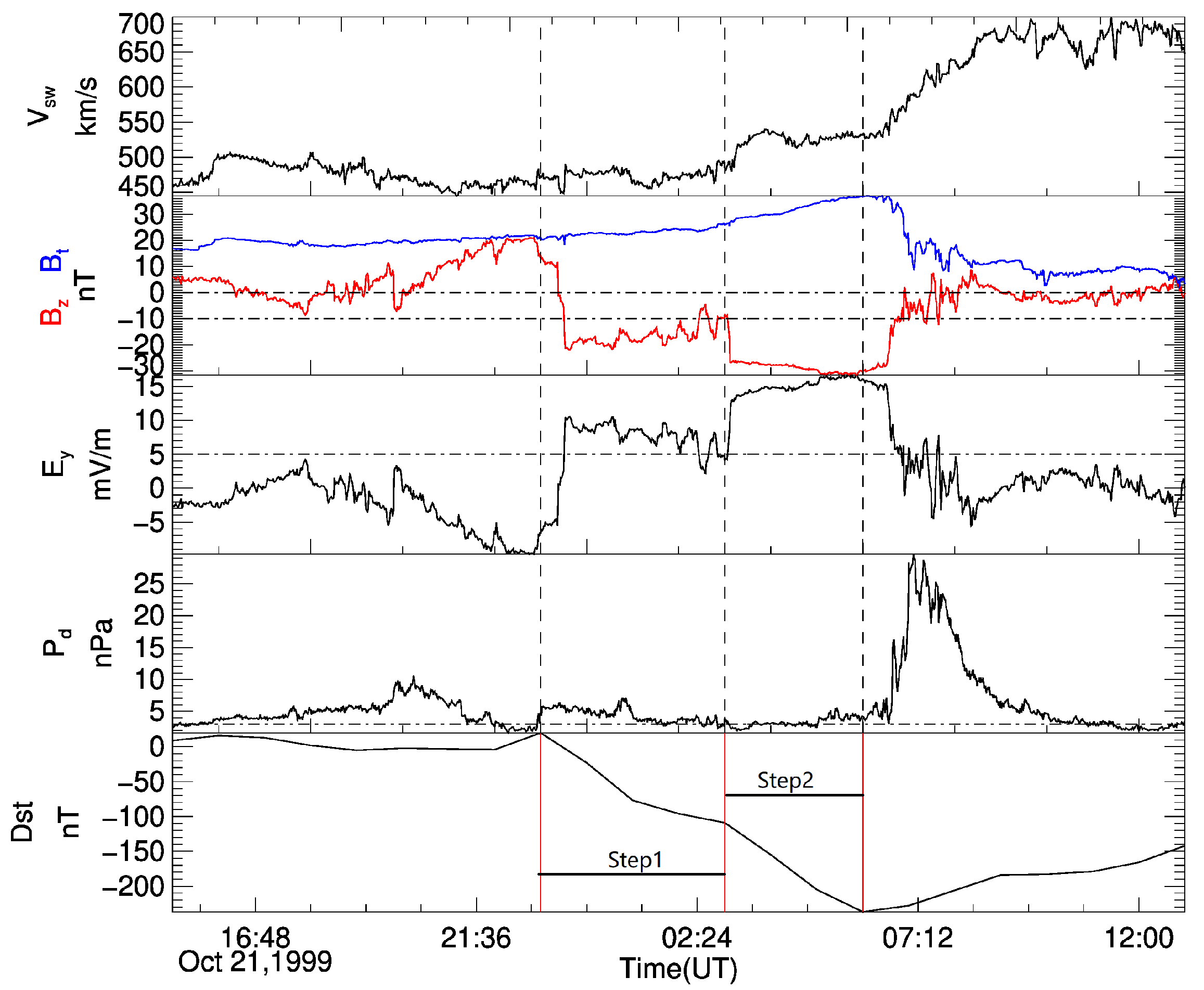
2.2. Why Should We Use the SYM-H Index?

The first question that should be answered is why we should use the SYM-H index rather than the Dst index to study the properties of the main phase of a storm. To answer this question, a comparison between the SYM-H index and the Dst index, along with the corresponding solar wind parameters, is made and shown in Figure 1. An IP shock reached the magnetosphere at 2:21 a.m. UT on 21 October 1999, indicated by the first vertical dashed line. The SYM-H index increased suddenly at 2:25 a.m. UT on 21 October 1999, indicated by the first vertical red solid line, suggesting that the magnetosphere took 4 min to respond to the IP shock. However, we could not find any sudden increase in the Dst index. The Dst index began to decrease continuously from 11:00 p.m. UT on 21 October 1999, which is indicated by the vertical green solid line shown in Figure 1. The Dst index reached its lowest value of 237 nT at 6:00 a.m. UT on 22 October 1999. It is evident that the start and end time of the storm’s main phase, determined by the Dst index, were 11:00 p.m. UT on 21 October 1999 and 6:00 a.m. UT on 22 October 1999, respectively. It is noted that the z-component of the IMF was still northward at 11:00 p.m. UT on 21 October 1999. The z-component of the IMF turned southward at 11:23 p.m. UT on 21 October 1999, as indicated by the second vertical dashed line shown in Figure 1. Hence, it is impossible that the start time of the main phase of the storm was earlier than 11:23 p.m. UT on 21 October 1999, namely due to the start time determined by the Dst index not being reasonable. The start time of the storm’s main phase described by the SYM-H index had to be later than 11:23 p.m. UT on 21 October 1999 because the SYM-H index should take some time to respond to the southward component of the IMF [42]. The SYM-H index began to decrease from 11:44 p.m. UT on 22 October 1999, indicating that the start time of the main phase of the storm determined by the SYM-H index was 11:44 p.m. UT. It is evident that the SYM-H index took 21 min to respond to the southward component of the IMF. Anyway, the variation of the SYM-H index over time fit the temporal of the solar wind parameters better than the Dst index, although there were some differences between the SYM-H index and the Dst index [43]. We can see from Figure 1 that rapid variation of the ring current of the storm could not be seen from the variation of the Dst index over time. On the contrary, the variation of the SYM-H index over time could provide information on the rapid variation of the ring current of the storm. This is the reason why we used the SYM-H index to analyze the properties of the geomagnetic storm’s main phase in this study.

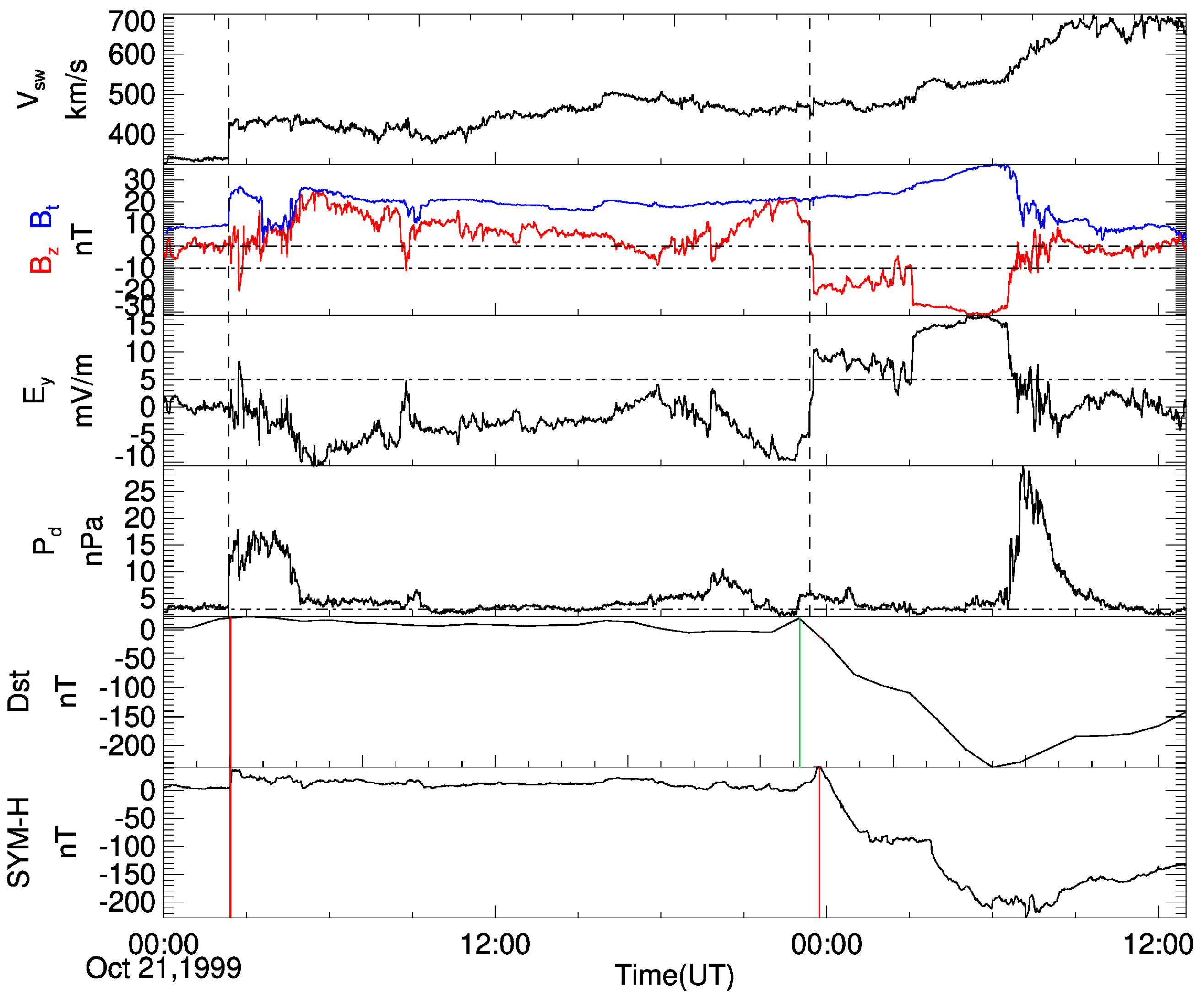
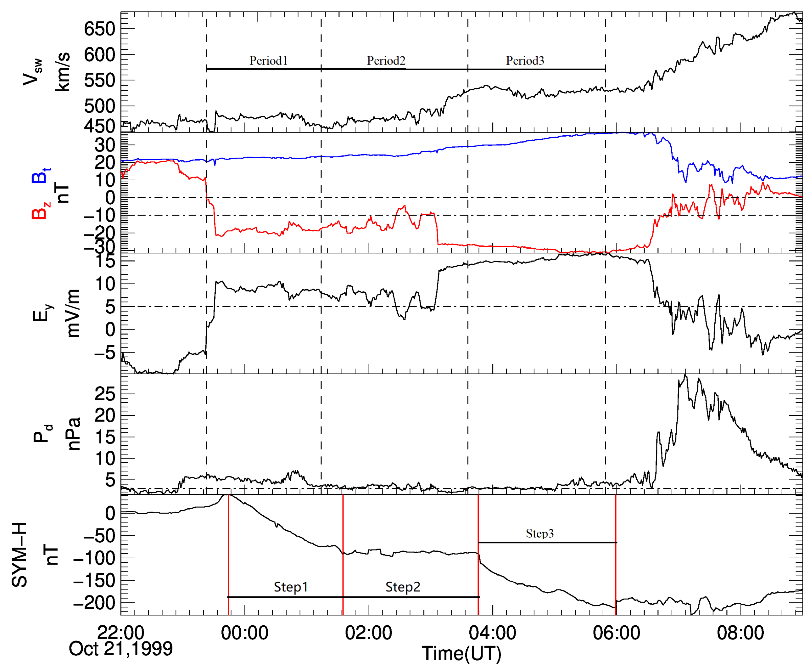
2.3. Properties of the Storm’s Main Phase

According to the variation in the SYM-H index during the storm’s main phase, we can easily find that the SYM-H index did not decrease in a sustained manner during the storm’s main phase, as shown in Figure 2. It is obvious that there were two periods during which the SYMH index decreased quickly. As shown in Figure 2, the SYM-H index decreased quickly during step 1 and step 3. The SYM-H index began to decrease continuously from the moment of 11:44 p.m. UT on 21 October 1999, which corresponds to the moment of 11:23 p.m. UT on 21 October 1999 when the z-component of the IMF turned southward. The time interval between 11:23 p.m. UT and 11:44 p.m. UT on 21 October 1999 is 21 min. The end time of step 1 was 1:35 a.m. UT on 22 October 1999, which corresponded to the solar wind time at 1:14 a.m. UT on 22 October 1999. Hence, the IP source responsible for step 1 was the solar wind during period 1 from 11:21 p.m. UT on 21 October 1999 to 1:14 a.m. UT on 22 October 1999. The start time of step 3 was 3:46 a.m. UT on 22 October 1999, when the SYM-H index began to decrease continuously again. The corresponding time of the solar wind should have been 3:36 a.m. UT on 22 October 1999 because the solar wind dynamic pressure started to be larger than 3 nPa. The time interval between the SYM-H index of step 3 and the solar wind of period 3 was 10 min. The end time of step 3 was 5:59 a.m. UT on 22 October 1999, and the corresponding time of the solar wind was determined to be 5:49 a.m. UT on 22 October 1999. The IP sources responsible for the variation in the SYM-H index during step 1 and step 3 were determined to be the solar wind during period 1 and period 3,respectively, as shown in Figure 2. To study the properties of the main phase of the storm during step 1 and step 3, the properties of the variation in the SYM-H index during the two steps will be calculated. The formula in Equation (7) in the article by Zhao et al. [31], which is listed below, will be used to calculate the real variation of the ring current during a period with the start time at t s and the end time at t e :
Δ S Y M H o b = S Y M H o b ( t e ) S Y M H o b ( t s ) + 7.26 P d | t s 7.26 P d | t e
where S Y M H o b is the observed SYM-H index, P d is the solar wind dynamic pressure, P d | t s and P d | t e are the P d at the times t s and t e , respectively, abd S Y M H o b is the pressure-corrected SYM-H index.
We set Δ t = t e t s , and then the averaged variation rate of the ring current during a period was calculated as shown below:
Δ S Y M H o b / Δ t
According to Equations (1) and (2), the derived Δ S Y M H o b and Δ S Y M H o b / Δ t during step 1 and step 3 are listed in Table 1. As shown in Table 1, | Δ S Y M H o b 1 | was larger than | Δ S Y M H o b 3 | , and | Δ S Y M H o b 1 / Δ t 1 | was larger than | Δ S Y M H o b 3 / Δ t 3 | .

2.4. Properties of the Solar Wind Parameters during Period 1 and Period 3

The time integrals of B s during period 1 and period 3 were calculated as shown below:
I ( B s ) = t 1 t 2 B s d t
where B s is the southward component of the IMF and t 1 and t 2 are the start and end times of the selected period, respectively. The averaged B s was calculated as shown below:
B s ¯ = I ( B s ) / Δ t
The time integrals of E y during period 1 and period 3 were calculated as shown below:
I ( E y ) = t 1 t 2 E y d t
where E y is the solar wind electric field and t 1 and t 2 are the start and end time of the selected period, respectively. The averaged E y was calculated as shown below:
E y ¯ = I ( E y ) / Δ t
The derived I ( B s ) and B s ¯ during period 1 and period 3, respectively, are listed in Table 2, while the derived I ( E y ) and E y ¯ are listed in Table 3. We can see from Table 2 that | I ( B s 1 ) | was smaller than | I ( B s 3 ) | , and | B s 1 ¯ | was smaller than | B s 3 ¯ | . In addition, | B s 1 m a x | was smaller than | B s 3 m a x | . As shown in Table 3, I ( E y 1 ) was smaller than I ( E y 3 ) , and E y 1 ¯ was smaller than E y 3 ¯ . In addition, E y 1 m a x was smaller than E y 3 m a x .
The time integrals of P d during period 1 and period 3 were calculated as shown below:
I ( P d ) = t 1 t 2 P d d t
where P d is the solar wind dynamic pressure and t 1 and t 2 are the start and end time of the selected period, respectively. The averaged P d was calculated as shown below:
P d ¯ = I ( P d ) / Δ t
The results of the calculation on the solar wind dynamic pressure are listed in Table 4.

3. Discussion

The magnetosphere took 4 min to respond to the IP shock in our study, which is basically consistent with the result that the propagation time of the disturbance produced by an IP shock from the Earth’s bow shock to the ground, such as SSC, which was 5 min as obtained in the article by Villante et al. [44]. If the z-component of the IMF turned from south to north, the magnetosphere took 28–44 min to respond to the corresponding disturbance caused by the solar wind, but the response time of the magnetosphere to the disturbance caused by the solar wind was 17–25 min for the events with the z-component of the IMF turning from north to south [45]. The z-component of the IMF in the present study was in a northward direction and then turned southward at 11:23 p.m. UT on 21 October 1999, as indicated by the first vertical dashed line shown in Figure 2. The time interval between the moment when the z-component of the IMF turned from north to south and the moment when the SYM-H index began to decrease continuously was 21 min, indicating that the response time of the SYM-H index to the southward component of the IMF was 21 min, which was consistent with the result that the lag time varied from 17 to 25 min for 5 cases with northward-to-southward turnings in the article by Hairston and Heelis [45]. The response of the magnetosphere to the disturbance caused by the solar wind is very complicated (e.g., [42,46,47,48,49,50] and the references therein). Many more studies should be conducted to understand the time lag between the disturbance caused by the solar wind and the magnetosphere better.
If the geomagnetic activity intensity is determined by the peak value of B s or E y , then the geomagnetic activity intensity caused by the solar wind during period 3 should be much stronger than that caused by the solar wind during period 1 because | B s 3 m a x | was larger than | B s 1 m a x | , E y 3 m a x was much larger than E y 1 m a x , and Δ t 3 was longer than Δ t 1 , which can be seen from Table 2 and Table 3. However, Δ S Y M H o b 1 was larger than Δ S Y M H o b 3 , indicating that the peak values of B s or E y were not the determining factors for the geomagnetic activity intensity. If the geomagnetic activity intensity depends on the time integral of the solar wind electric field, then the geomagnetic activity intensity caused by the solar wind during period 3 should be much stronger than that caused by the solar wind during period 1, because I ( E y 3 ) was much larger than I ( E y 1 ) . However, Δ S Y M H o b 1 was larger than Δ S Y M H o b 3 , indicating that the geomagnetic activity intensity was not determined by the time integral of the solar wind electric field either. What is the reason for this? We found that the solar wind dynamic pressure during period 1 was larger than that during period 3, as shown in Table 4. This is strong evidence that the solar wind dynamic pressure is an important factor for the geomagnetic activity intensity along with the solar wind speed and B s . In this context, the empirical formulae that the intensity of a geomagnetic storm completely depends on the peak value of B s , created by Gopalswamy et al. [23,24], or the empirical formula created by Shen et al. [25] have no physical meaning, because these formulae cannot reflect the sustained interaction between the solar wind and magnetosphere, and the contribution given by the solar wind dynamic pressure is neglected. As a matter of fact, some researchers have realized that the solar wind dynamic pressure may be important for the geomagnetic storm intensity. For example, Yermolaev et al. [51,52,53] suggested that sheath compression regions usually have a higher speed and higher dynamic pressure and therefore have a higher geomagnetic efficiency than magnetic clouds, implying that the solar wind dynamic pressure is an important parameter for the intensity of a geomagnetic storm.
We may need to adjust the start time and end time for the solar wind during period 1 and period 3 a little so that the IP source responsible for the variations in the SYM-H index during step 1 and step 3 are completely accurate. However, | Δ S Y M H o b 1 | / Δ t 1 was larger than | Δ S Y M H o b 3 / Δ t 3 | , ensuring that the solar wind responsible for Δ S Y M H o b 1 had a higher geomagnetic efficiency than that responsible for Δ S Y M H o b 3 .
The variation in the SYM-H index during step 2, shown in Figure 2, was very small, indicating that the injection term was almost equal to the decay term of the ring current. Therefore, we did not study the properties of the solar wind parameters during period 2, which was responsible for the variation in the SYM-H index during step 2.
It should be noted that the main phase of the geomagnetic storm and the corresponding solar wind parameters for if we used the Dst index are shown in Figure 3. The main phase of the storm was constituted by step 1 and step 2. We used Δ D s t 1 and Δ D s t 2 to indicate the variation in the Dst index during step 1 and step 2, respectively, and we used Δ t 1 and Δ t 2 to indicate the duration of step 1 and step 2, respectively. The first, second and third vertical red solid lines stand for the moments of 11:00 p.m. UT on 21 October 1999, 3:00 a.m. UT on 22 October 1999 and 6:00 a.m. UT on 22 October 1999, respectively. Hence, Δ t 1 was equal to 4 h, while Δ t 2 was equal to 3 h. According to the Dst index, the value was 20 nT at 11:00 p.m. UT on 21 October 1999, while the value was 109 nT at 3:00 a.m. UT on 22 October 1999. Hence, the Δ D s t 1 was 129 nT. Similarly, Δ D s t 2 was 128 nT. However, | Δ D s t 2 / Δ t 2 | > | Δ D s t 1 / Δ t 1 | , namely because the Dst index decreased more rapidly during step 2 than during step 1. The Z-component of the IMF changed from 8.72 nT at 3:03 a.m. UT to 26.61 nT at 3:07 a.m. UT. Hence, the hourly averaged z-component of the IMF responsible for the variation in the Dst index during step 2 was much larger than that responsible for the variation in the Dst index during step 1. Because the z-component of the IMF during step 2 was much larger than that during step 1, this may be the reason why Dal Lago et al. [40] concluded that the larger value for B s led to the Dst index decreasing more rapidly during step 2 and that a larger B s value had higher geomagnetic efficiency. This tells us that if we use the Dst index in this case study, we cannot find the truth in how the solar wind dynamic pressure plays an important role in the geomagnetic activity’s intensity.

4. Summary and Conclusions

We studied the properties of the main phase of the geomagnetic storm that occurred on 21–22 October 1999 and then compared them with the corresponding solar wind parameters. The results are summarized below:
(1) The main phase of the geomagnetic storm that occurred on 1999 October 21–22 was split into three steps. The SYM-H index decreased quickly during step 1 and step 3, while the variation in the SYM-H index during step 2 was very small. The IP source responsible for the SYM-H index during step 1 and step 3 was the solar wind during period 1 and period 3, respectively. We found that | B s 3 m a x | was larger than | B s 1 m a x | , E y 3 m a x was larger than E y 1 m a x , and Δ t 3 was longer than Δ t 1 . However, Δ S Y M H o b 1 was larger than Δ S Y M H o b 3 , indicating that the CC between the intensity of a geomagnetic storm and the largest southward component of the IMF or the CC between the intensity of a geomagnetic storm and the largest solar wind electric field had no physical meaning. I ( E y 1 ) was smaller than I ( E y 3 ) . However, Δ S Y M H o b 1 was larger than Δ S Y M H o b 3 , indicating that the CC between the intensity of a geomagnetic storm and the time integral of the solar wind electric field during the main phase of the storm was incomplete. The reason that Δ S Y M H o b 1 was larger than Δ S Y M H o b 3 is that the solar wind dynamic pressure during period 1 was larger than that during period 3. This is evidence that the solar wind dynamic pressure is an important parameter for determining the intensity of a geomagnetic storm, along with the solar wind speed and the southward component of the IMF.
(2) The magnetosphere took 4 min to respond to the IP shock. The time lag between the moment when the z-component of the IMF turned from north to south and the moment when the SYM-H index began to decrease continuously was 21 min.

Author Contributions

Q.L. prepared the solar wind and geomagnetic data and wrote the original draft of the manuscript in Word format; M.-X.Z. wrote the IDL program to show the variation in the solar wind and the geomagnetic data over time, made the calculations needed for the study and compiled the draft of the manuscript with LaTeX; G.-M.L. provided the idea and checked and revised the manuscript in LaTeX format; all authors took part in, discussed and agreed upon the results of the calculations. All authors have read and agreed to the published version of the manuscript.

Funding

This research was funded by the Sino-South Africa Joint Research on Polar Space Environment (2021YFE0106400), International Cooperation Project on Scientific and Technological Innovation Between Governments, National Key Plans on Research and Development, Ministry of Science and Technology of China, the Special Fund of the Institute of Geophysics, China Earthquake Administration (Grant Number DQJB21X26), CAS Key Laboratory of Solar Activity under number KLSA202109 and the National Natural Science Foundation of China (grant numbers 41074132, 41474166, 41774195 and 41774085).

Institutional Review Board Statement

Not applicable.

Informed Consent Statement

Not applicable.

Data Availability Statement

We acknowledge the use of NASA and GSFC’s Space Physics Data Facility’s OMNI data and web service (https://omniweb.gsfc.nasa.gov/html/omni_min_data.html, accessed on 27 April 2022). We also thank the Center for Geomagnetism and Space Magnetism at Kyoto University for providing the Dst and SYM-H indexes.

Conflicts of Interest

The authors declare no conflict of interest.

References

  1. Ganushkina, N.; Jaynes, A.; Liemohn, M. Space Weather Effects Produced by the Ring Current Particles. Space Sci. Rev. 2017, 212, 1315–1344. [Google Scholar] [CrossRef] [Green Version]
  2. Dungey, J.W. Interplanetary Magnetic Field and the Auroral Zones. Phys. Rev. Lett. 1961, 6, 47–48. [Google Scholar] [CrossRef]
  3. Gonzalez, W.D.; Tsurutani, B.T.; Clúa de Gonzalez, A.L. Interplanetary origin of geomagnetic storms. Space Sci. Rev. 1999, 88, 529–562. [Google Scholar] [CrossRef]
  4. Riley, P.; Baker, D.; Liu, Y.D.; Verronen, P.; Singer, H.; Güdel, M. Extreme Space Weather Events: From Cradle to Grave. Space Sci. Rev. 2017, 214, 21. [Google Scholar] [CrossRef]
  5. Alves, M.V.; Echer, E.; Gonzalez, W.D. Geoeffectiveness of corotating interaction regions as measured by Dst index. J. Geophys. Res. Space Phys. 2006, 111, A07S05. [Google Scholar] [CrossRef] [Green Version]
  6. Gonzalez, W.D.; Echer, E.; Clua-Gonzalez, A.L.; Tsurutani, B.T. Interplanetary origin of intense geomagnetic storms (Dst < −100 nT) during solar cycle 23. Geophys. Res. Lett. 2007, 34. [Google Scholar] [CrossRef] [Green Version]
  7. Echer, E.; Gonzalez, W.D.; Tsurutani, B.T.; Gonzalez, A.L.C. Interplanetary conditions causing intense geomagnetic storms (Dst ≤ −100 nT) during solar cycle 23 (1996–2006). J. Geophys. Res. Space Phys. 2008, 113, A05221. [Google Scholar] [CrossRef]
  8. Zhang, Y.; Sun, W.; Feng, X.S.; Deehr, C.S.; Fry, C.D.; Dryer, M. Statistical analysis of corotating interaction regions and their geoeffectiveness during solar cycle 23. J. Geophys. Res. Space Phys. 2008, 113, A08106. [Google Scholar] [CrossRef]
  9. Choi, Y.; Moon, Y.J.; Choi, S.; Baek, J.H.; Kim, S.S.; Cho, K.S.; Choe, G.S. Statistical Analysis of the Relationships among Coronal Holes, Corotating Interaction Regions, and Geomagnetic Storms. Sol. Phys. 2009, 254, 311–323. [Google Scholar] [CrossRef]
  10. Gupta, V.; Badruddin. Interplanetary structures and solar wind behaviour during major geomagnetic perturbations. J. Atmos. Sol.-Terr. Phys. 2009, 71, 885–896. [Google Scholar] [CrossRef]
  11. Ji, E.Y.; Moon, Y.J.; Kim, K.H.; Lee, D.H. Statistical comparison of interplanetary conditions causing intense geomagnetic storms (Dst ≤ −100 nT). J. Geophys. Res. Space Phys. 2010, 115, A10232. [Google Scholar] [CrossRef] [Green Version]
  12. Kane, R. Relationship between the geomagnetic Dst(min) and the interplanetary Bz(min) during cycle 23. Planet. Space Sci. 2010, 58, 392–400. [Google Scholar] [CrossRef]
  13. Joshi, N.C.; Bankoti, N.S.; Pande, S.; Pande, B.; Pandey, K. Relationship between interplanetary field/plasma parameters with geomagnetic indices and their behavior during intense geomagnetic storms. New Astron. 2011, 16, 366–385. [Google Scholar] [CrossRef]
  14. Echer, E.; Tsurutani, B.T.; Gonzalez, W.D. Interplanetary origins of moderate (−100 nT < Dst ≤ −50 nT) geomagnetic storms during solar cycle 23 (1996–2008). J. Geophys. Res. Space Phys. 2013, 118, 385–392. [Google Scholar] [CrossRef] [Green Version]
  15. Richardson, I.G.; Cane, H.V. Near-Earth Interplanetary Coronal Mass Ejections During Solar Cycle 23 (1996–2009): Catalog and Summary of Properties. Sol. Phys. 2010, 264, 189–237. [Google Scholar] [CrossRef]
  16. Richardson, I.G. Geomagnetic activity during the rising phase of solar cycle 24. J. Space Weather Space Clim. 2013, 3, A08. [Google Scholar] [CrossRef] [Green Version]
  17. Wu, C.C.; Lepping, R.P. Relationships Among Geomagnetic Storms, Interplanetary Shocks, Magnetic Clouds, and Sunspot Number During 1995–2012. Sol. Phys. 2016, 291, 265–284. [Google Scholar] [CrossRef]
  18. Badruddin, A.; Falak, Z. Study of the geoeffectiveness of coronal mass ejections, corotating interaction regions and their associated structures observed during Solar Cycle 23. Astrophys. Space Sci. 2016, 361, 253. [Google Scholar] [CrossRef]
  19. Goswami, A. Difference in the parameters of ICMEs in Ejecta and Sheath region and their impact on Dst index during 1997–2014. Adv. Space Res. 2018, 62, 692–706. [Google Scholar] [CrossRef]
  20. Lawrance, M.; Moon, Y.; Shanmugaraju, A. Relationships between Interplanetary Coronal Mass Ejection Characteristics and Geoeffectiveness in the Declining Phase of Solar Cycles 23 and 24. Sol. Phys. 2020, 295, 62. [Google Scholar] [CrossRef]
  21. Balachandran, R.; Chen, L.J.; Wang, S.; Fok, M.C. Correlating the interplanetary factors to distinguish extreme and major geomagnetic storms. Earth Planet. Phys. 2021, 5, 180. [Google Scholar] [CrossRef]
  22. Hajra, R.; Sunny, J.V. Corotating Interaction Regions during Solar Cycle 24: A Study on Characteristics and Geoeffectiveness. Sol. Phys. 2022, 297, 30. [Google Scholar] [CrossRef]
  23. Gopalswamy, N. Solar connections of geoeffective magnetic structures. J. Atmos. Sol.-Terr. Phys. 2008, 70, 2078–2100. [Google Scholar] [CrossRef]
  24. Gopalswamy, N.; Akiyama, S.; Yashiro, S.; Michalek, G.; Lepping, R. Solar sources and geospace consequences of interplanetary magnetic clouds observed during solar cycle 23. J. Atmos.-Sol.-Terr. Phys. 2008, 70, 245–253. [Google Scholar] [CrossRef]
  25. Shen, C.; Chi, Y.; Wang, Y.; Xu, M.; Wang, S. Statistical comparison of the ICME’s geoeffectiveness of different types and different solar phases from 1995 to 2014. J. Geophys. Res. Space Phys. 2017, 122, 5931–5948. [Google Scholar] [CrossRef]
  26. Burton, R.K.; McPherron, R.L.; Russell, C.T. An empirical relationship between interplanetary conditions and Dst. J. Geophys. Res. (1896–1977) 1975, 80, 4204–4214. [Google Scholar] [CrossRef]
  27. O’Brien, T.P.; McPherron, R.L. An empirical phase space analysis of ring current dynamics: Solar wind control of injection and decay. J. Geophys. Res. Space Phys. 2000, 105, 7707–7719. [Google Scholar] [CrossRef]
  28. Lee, J.O.; Cho, K.S.; Kim, R.S.; Jang, S.; Marubashi, K. Effects of Geometries and Substructures of ICMEs on Geomagnetic Storms. Sol. Phys. 2018, 293, 129. [Google Scholar] [CrossRef]
  29. Le, G.M.; Liu, G.A.; Zhao, M.X. Dependence of Major Geomagnetic Storm Intensity (Dst ≤ −100 nT) on Associated Solar Wind Parameters. Sol. Phys. 2020, 295, 108. [Google Scholar] [CrossRef]
  30. Zhao, M.X.; Le, G.M.; Li, Q.; Liu, G.A.; Mao, T. Dependence of Great Geomagnetic Storm (ΔSYM-H ≤ −200nT) on Associated Solar Wind Parameters. Sol. Phys. 2021, 296, 66. [Google Scholar] [CrossRef]
  31. Zhao, M.X.; Le, G.M.; Lu, J. Can We Estimate the Intensities of Great Geomagnetic Storms (ΔSYM-H ≤ −200 nT) with the Burton Equation or the O’Brien and McPherron Equation? Astrophys. J. 2022, 928, 18. [Google Scholar] [CrossRef]
  32. Wang, C.B.; Chao, J.K.; Lin, C.H. Influence of the solar wind dynamic pressure on the decay and injection of the ring current. J. Geophys. Res. Space Phys. 2003, 108, 1341. [Google Scholar] [CrossRef]
  33. Kataoka, R.; Miyoshi, Y. Magnetosphere inflation during the recovery phase of geomagnetic storms as an excellent magnetic confinement of killer electrons. Geophys. Res. Lett. 2008, 35, L06S09. [Google Scholar] [CrossRef] [Green Version]
  34. Liu, G.A.; Zhao, M.X.; Le, G.M.; Mao, T. What Can We Learn from the Geoeffectiveness of the Magnetic Cloud on 2012 July 15–17? Res. Astron. Astrophys. 2022, 22, 015002. [Google Scholar] [CrossRef]
  35. Cheng, L.B.; Le, G.M.; Zhao, M.X. Sun-Earth connection event of super geomagnetic storm on 2001 March 31: The importance of solar wind density. Res. Astron. Astrophys. 2020, 20, 036. [Google Scholar] [CrossRef] [Green Version]
  36. Richardson, I.G.; Webb, D.F.; Zhang, J.; Berdichevsky, D.B.; Biesecker, D.A.; Kasper, J.C.; Kataoka, R.; Steinberg, J.T.; Thompson, B.J.; Wu, C.C.; et al. Major geomagnetic storms (Dst ≤ −100 nT) generated by corotating interaction regions. J. Geophys. Res. Space Phys. 2006, 111, A07S09. [Google Scholar] [CrossRef]
  37. Le, G.M.; Zhao, M.X.; Zhang, W.T.; Liu, G.A. Source Locations and Solar-Cycle Distribution of the Major Geomagnetic Storms (Dst ≤ −100 nT) from 1932 to 2018. Sol. Phys. 2021, 296, 187. [Google Scholar] [CrossRef]
  38. Le, G.M.; Zhang, Y.N.; Zhao, M.X. Statistical and Solar Cycle Distribution of Daily Flux ≥ 109 cm−2 d−1 sr−1 for E > 2MeV Electrons Observed by GOES During 1987-2019. Sol. Phys. 2021, 296, 16. [Google Scholar] [CrossRef]
  39. Zhang, J.; Richardson, I.G.; Webb, D.F.; Gopalswamy, N.; Huttunen, E.; Kasper, J.C.; Nitta, N.V.; Poomvises, W.; Thompson, B.J.; Wu, C.C.; et al. Solar and interplanetary sources of major geomagnetic storms (Dst ≤ −100 nT) during 1996–2005. J. Geophys. Res. Space Phys. 2007, 112, A10102. [Google Scholar] [CrossRef] [Green Version]
  40. Dal Lago, A.; Gonzalez, W.D.; Balmaceda, L.A.; Vieira, L.E.A.; Echer, E.; Guarnieri, F.L.; Santos, J.; da Silva, M.R.; de Lucas, A.; Clua de Gonzalez, A.L.; et al. The 17–22 October (1999) solar-interplanetary-geomagnetic event: Very intense geomagnetic storm associated with a pressure balance between interplanetary coronal mass ejection and a high-speed stream. J. Geophys. Res. Space Phys. 2006, 111, A07S14. [Google Scholar] [CrossRef] [Green Version]
  41. Wanliss, J.A.; Showalter, K.M. High-resolution global storm index: Dst versus SYM-H. J. Geophys. Res. Space Phys. 2006, 111, A02202. [Google Scholar] [CrossRef]
  42. Maggiolo, R.; Hamrin, M.; De Keyser, J.; Pitkänen, T.; Cessateur, G.; Gunell, H.; Maes, L. The Delayed Time Response of Geomagnetic Activity to the Solar Wind. J. Geophys. Res. Space Phys. 2017, 122, 11109–11127. [Google Scholar] [CrossRef] [Green Version]
  43. Katus, R.M.; Liemohn, M.W. Similarities and differences in low- to middle-latitude geomagnetic indices. J. Geophys. Res. Space Phys. 2013, 118, 5149–5156. [Google Scholar] [CrossRef] [Green Version]
  44. Villante, U.; Lepidi, S.; Francia, P.; Bruno, T. Some aspects of the interaction of interplanetary shocks with the Earth’s magnetosphere: An estimate of the propagation time through the magnetosheath. J. Atmos. Sol.-Terr. Phys. 2004, 66, 337–341. [Google Scholar] [CrossRef]
  45. Hairston, M.R.; Heelis, R.A. Response time of the polar ionospheric convection pattern to changes in the north-south direction of the IMF. Geophys. Res. Lett. 1995, 22, 631–634. [Google Scholar] [CrossRef]
  46. Andréeová, K. The study of instabilities in the solar wind and magnetosheath and their interaction with the Earth’s magnetosphere. Planet. Space Sci. 2009, 57, 888–890. [Google Scholar] [CrossRef]
  47. Farrugia, C.; Freeman, M.; Cowley, S.; Southwood, D.; Lockwood, M.; Etemadi, A. Pressure-driven magnetopause motions and attendant response on the ground. Planet. Space Sci. 1989, 37, 589–607. [Google Scholar] [CrossRef]
  48. Koval, A.; Šafránková, J.; Němeček, Z.; Samsonov, A.A.; Přech, L.; Richardson, J.D.; Hayosh, M. Interplanetary shock in the magnetosheath: Comparison of experimental data with MHD modeling. Geophys. Res. Lett. 2006, 33, L11102. [Google Scholar] [CrossRef]
  49. Safargaleev, V.; Kozlovsky, A.; Honary, F.; Voronin, A.; Turunen, T. Geomagnetic disturbances on ground associated with particle precipitation during SC. Ann. Geophys. 2010, 28, 247–265. [Google Scholar] [CrossRef] [Green Version]
  50. Samsonov, A.A.; Sibeck, D.G.; Dmitrieva, N.P.; Semenov, V.S. What Happens Before a Southward IMF Turning Reaches the Magnetopause? Geophys. Res. Lett. 2017, 44, 9159–9166. [Google Scholar] [CrossRef] [Green Version]
  51. Yermolaev, Y.I.; Nikolaeva, N.S.; Lodkina, I.G.; Yermolaev, M.Y. Specific interplanetary conditions for CIR-, Sheath-, and ICME-induced geomagnetic storms obtained by double superposed epoch analysis. Ann. Geophys. 2010, 28, 2177–2186. [Google Scholar] [CrossRef] [Green Version]
  52. Yermolaev, Y.I.; Nikolaeva, N.S.; Lodkina, I.G.; Yermolaev, M.Y. Geoeffectiveness and efficiency of CIR, sheath, and ICME in generation of magnetic storms. J. Geophys. Res. Space Phys. 2012, 117, A00L07. [Google Scholar] [CrossRef] [Green Version]
  53. Yermolaev, Y.I.; Lodkina, I.G.; Dremukhina, L.A.; Yermolaev, M.Y.; Khokhlachev, A.A. What Solar–Terrestrial Link Researchers Should Know about Interplanetary Drivers. Universe 2021, 7, 138. [Google Scholar] [CrossRef]
Figure 1. The comparison between the Dst index and the SYM-H index as well as the corresponding solar wind parameters during the period from 12:00 a.m. UT on 21 October 1999 to 1:00 p.m. UT on 22 October 1999. From top to bottom are solar wind speed, the total strength of the IMF ( B t ), indicated by blue solid line, the z-component of the IMF, indicated by the red solid line ( B z ), the solar wind electric field ( E y ), solar wind dynamic pressure ( P d ), Dst index and SYM-H index. The first vertical dashed line indicates the moment that the IP shock reached the magnetosphere. The first vertical red solid line indicates the moment when the SYM-H index increased suddenly. The second vertical dashed line indicates the moment when the z-component of the IMF began to be directed southward. The vertical green solid line indicates the moment when the Dst index began to decrease. The vertical red solid line indicates the moment when the SYM-H index began to decrease. The two horizontal dot-dashed lines in the second panel denote 0 and 10 nT. The dot-dashed line in the third panel indicates 5 mV/m. The dot-dashed line in the fourth panel indicates 3 nPa.
Universe 08 00346 g001
Figure 2. Solar wind parameters and SYM-H index from 10:00 p.m. UT on 21 October 1999 to 9:00 a.m. UT on 22 October 1999. Period 1 started at 11:23 p.m. UT on 21 October and ended at 1:14 a.m. UT on 22 October. Step 1 started at 11:44 p.m. UT on 21 October and ended at 1:35 a.m. UT on 22 October. Period 3 started at 3:33 a.m. UT and ended at 5:46 a.m. UT on 22 October. Step 3 started at 3:46 a.m. UT and ended at 5:49 a.m. UT on 22 October.
Universe 08 00346 g002
Figure 3. Solar wind parameters and Dst index from 3:00 p.m. UT on 21 October 1999 to 1:00 p.m. UT on 22 October 1999. The first vertical dashed and red solid lines stand for the moment of 11:00 p.m. UT on 21 October 1999. The second vertical dashed and red solid lines represent the moment of 3:00 a.m. UT on 22 October 1999. The third vertical dashed and red solid lines signify the moment of 6:00 a.m. UT on 22 October 1999.
Universe 08 00346 g003
Table 1. Δ S Y M H o b and Δ S Y M H o b / Δ t during step 1 and step 3.
Step 1Step 3
(11:44 p.m. 21 October ∼ 1:35 a.m. 22 October)(3:46 a.m. ∼ 5:59 a.m. 22 October)
Δ SYMH ob 1 Δ t 1 Δ SYMH ob 1 / Δ t 1 Δ SYMH ob 3 Δ t 3 Δ SYMH ob 3 / Δ t 3
(nT)(min)(nT/min)(nT)(min)(nT/min)
−136.23111−1.23−124.88133−0.94
Table 2. The derived I ( B s ) , B s ¯ and B s m a x during period 1 and period 3.
Period 1Period 3
(11:23 p.m. 21 October ∼ 1:14 a.m. 22 October)(3:36 a.m. ∼ 5:49 a.m. 22 October)
I ( B s 1 ) Δ t 1 B s 1 ¯ B s 1 max I ( B s 3 ) Δ t 3 B s 3 ¯ B s 3 max
(nT·min)(min)(nT)(nT)(nT·min)(min)(nT)(nT)
−1962.67111−17.52−21.93−3898.09133−29.09−31.45
Table 3. The derived I ( E y ) , E y ¯ and E y m a x during period 1 and period 3.
Period 1Period 3
(11:23 p.m. 21 October ∼ 1:14 a.m. 22 October)(3:36 a.m. ∼ 5:49 a.m. 22 October)
I ( E y 1 ) Δ t 1 E y 1 ¯ E y 1 max I ( E y 3 ) Δ t 3 E y 3 ¯ E y 3 max
(mV/m·min)(min)(mV/m)(mV/m)(mV/m·min)(min)(mV/m)(mV/m)
934.371118.3410.552059.5413315.3716.71
Table 4. The derived I ( P d ) , P d ¯ and P d m a x during period 1 and period 3.
Period 1Period 3
(11:23 p.m. 21 October ∼ 1:14 a.m. 22 October)(3:36 a.m. ∼ 5:49 a.m. 22 October)
I ( P d 1 ) Δ t 1 P d 1 ¯ P d 1 max I ( P d 3 ) Δ t 3 P d 3 ¯ P d 3 max
(nPa·min)(min)(nPa)(nPa)(nPa·min)(min)(nPa)(nPa)
564.261115.047.07457.871333.425.52
Publisher’s Note: MDPI stays neutral with regard to jurisdictional claims in published maps and institutional affiliations.

