Abstract
A model capable of reproducing a set of solar wind parameters along the virtual spacecraft orbit out of an ecliptic plane has been developed. In the framework of a quasi-stationary axisymmetric self-consistent MHD model the spatial distributions of magnetic field and plasma characteristics at distances from 20 to 1200 Solar radii at almost all solar latitudes could be obtained and analyzed. This model takes into account the Sun’s magnetic field evolution during the solar cycle, when the dominant dipole magnetic field is replaced by the quadrupole one. Self-consistent solutions for solar wind characteristics were obtained, depending on the phase of the solar cycle. To verify the model, its results are compared with the observed characteristics of solar wind along the Ulysses trajectory during its flyby around the Sun from 1990 to 2009. It is shown that the results of numerical simulation are generally consistent with the observational data obtained by the Ulysses spacecraft. A comparison of the model and experimental data confirms that the model can adequately describe the solar wind parameters and can be used for heliospheric studies at different phases of the solar activity cycle, as well as in a wide range of latitudinal angles and distances to the Sun.
1. Introduction
The solar corona is the source of the solar wind (SW), which represents accelerated supersonic plasma flow with a frozen-in magnetic field (e.g., [1,2,3,4,5]). The interplanetary magnetic field (IMF) in the SW has a nonstationary turbulent character [6,7]. Various instabilities accompanied by the processes of magnetic reconnection [8,9,10,11,12], formation of magnetic islands and particle energization (e.g., [13]) can develop in this active media. Moreover, the role of various kinetic microinstabilities in the turbulent regions behind shock waves propagating in the solar wind can be substantial in a formation of a strong proton temperature anisotropy in solar wind plasma [14,15,16,17].
If one averages the observational data over time intervals much larger than the solar rotation period, the large-scale quasi-stationary structures appear in the SW flow shaping the heliosphere into a whole system, including the bow and terminal shock waves, heliopause, heliosheath, and the heliospheric current sheet (HCS) [18,19,20,21]. Satellite observations indicate that the HCS having a thickness of about 104 km is embedded within a relatively thick heliospheric plasma sheet (HPS) with a thickness of about several solar radii [22]. At the intersection of HCS the magnetic flux extended from the Sun’s corona changes its sign. Recent experimental observations have shown that HCS has a complex internal structure [8,23,24,25] and is surrounded by relatively thin current sheets, in which proton dynamics is quasi-adiabatic, and the scale of magnetic inhomogeneity is comparable to ion gyroradii [26,27,28]. During the Earth’s motion in the ecliptic plane our planet crosses the folds of HCS, as a result, spacecraft in Earth’s vicinity register the intersections of the sector structures of the IMF with multidirectional magnetic fluxes [29,30]. Due to the cross-section of magnetic sectors, the structure of HCS and HPS at low latitudes is better investigated in comparison with high latitudes.
High-latitude regions of the heliosphere remained almost unexplored until the launch of the Ulysses spacecraft (1990–2009), whose main purpose was to measure the physical characteristics of the Sun’s polar regions (e.g., [31]). Ulysses remains the only spacecraft that traversed along a heliocentric orbit almost perpendicular to the ecliptic plane. This made it possible to investigate the properties of SW at high latitudes and in the circumpolar regions [32,33].
SW modeling is the effective method for studying the heliosphere and interpreting the available experimental observations. Theoretical models of the heliosphere began to develop after works of Vsekhsvyatsky et al. [34], Bondi [2], and Parker [1,35], in which pioneering hypotheses were made about the non-equilibrium nature of the solar amosphere and its expansion into the surrounding space. The most consistent in theoretical terms was Parker’s simple model of SW acceleration [1] to supersonic flow moving at a speed of 300–700 km/s. Several years later the results of the measurements by the Luna-2,3, Mariner-2, and Venus-spacecraft brilliantly confirmed the model assumptions and main results [3,36,37].
Since the cycle of Sun activity (so called Hale 22-years cycle) is accompanied by the heliomagnetic field evolution from dipole configuration (in the solar minimum) to a quadrupole one (with higher-order multipoles in the solar maximum), it is important to study the changes of heliosphere that influence the plasma structure of the solar system. At present, a relatively small number of publications have been devoted to SW modeling taking into account the cyclic change of the heliomagnetic field. Most of them are semi-empirical, non self-consistent and based on the method of the potential source surface [38,39]. Some models allow us to predict the presence of more than one large-scale current sheet in the heliosphere, along with the HCS, during the periods of significant non-dipolarity of the Sun’s magnetic field (e.g., [40,41,42,43,44,45]).
Along with the source surface models, MHD modeling is an effective method for describing SW structure and dynamics, which makes it possible to study self-consistent magneto-plasma structures and SW characteristics in the heliosphere (e.g., [46,47,48,49,50,51]). In some MHD models, the solar synoptic maps of photospheric magnetic fields are used as a boundary condition and three-dimensional MHD simulations, including non-stationary ones, are performed. Such models are effective for the modeling of complex structures, and correspondingly they strongly depend on the initial conditions (e.g., [52]). Today, there is a need to study the general SW structure and solve questions about the mechanisms of HCS and HPS formation, SW latitudinal heterogeneity, and investigations of transition region from the slow SW at low latitudes to the fast one at high latitudes, as well as characteristics of the SW at high latitudes at different phases of solar activity.
The development of adequate models describing SW is an important and still not entirely solved task. These models can also provide useful and effective methods to investigate the distant regions of the Sun environment where the information from spacecraft is scarce or not sufficient. Recently, Kim et al. [53] developed a time-dependent 3D MHD model of SW flow from 1 to 80 AU where protons and neutral hydrogen atoms are described in a frame of the two-fluid approach. The daily averages of the SW parameters were used to reproduce time-dependent effects. The model results have been compared with the data from three spacecraft: Ulysses, Voyager, and New Horizons. It was shown that this model, with 1 day averaging, is basically in agreement with spacecraft data, but during the years of the solar maxima, the discrepancy of model results and Ulysses data can be substantial due to intense coronal ejections supporting strong noises in 1 day averaged data series.
The aim of our work is to develop and verify the axisymmetric stationary MHD model of the SW presented earlier in [54,55], where discrete heliospheric configurations corresponding to different states of a heliomagnetic field at certain phases of the solar cycle are calculated. The model aimed to compare the model data of the SW with the observational data along the Ulysses spacecraft trajectory. In the model, we used 25.6 days averages of observational data, that allow the investigation of large-scale spatial and temporal effects in the SW flow. Our choice of such a simple 2D axisymmetrical MHD model is based on the standard [56] approach. We try to describe the averaged structure of the SW and its evolution during the solar activity cycle. In such a formulation of the problem the tilt of the magnetic dipole and other 3D effects could be neglected. On the considered large scale of the SW, we assumed that protons and electrons move as a single fluid flow; thus, a single-fluid approximation was used. Therefore, we are interested the most general characteristic of SW structure and consider the stationary model with different boundary conditions (snapshots), corresponding to multipole evolution of the heliomagnetic field. Non-stationary effects occurring in the SW, such as mass ejections, plasma turbulence, instabilities and plasma acceleration were not taken into account in this averaged approach, although they may be very important and interesting in other investigations. The assessment of SW states at different phases of the solar activity cycle should allow us to answer the question as to what extent the proposed model is consistent with in situ observations of the SW. Consequently, this should, in turn, show to what extent our model can be applied to describe the large-scale structure of the SW in such domains of the heliosphere that are currently inaccessible for current and planned space missions.
2. Ulysses Data and Modeling
2.1. Flight of the Ulysses Spacecraft
Ulysses [57], launched in 1990, is a unique spacecraft that circled the Sun three times over its Northern and Southern poles. After passing near Jupiter in 1992, the spacecraft moved along a heliocentric orbit located at a distance from the Sun at perihelion about 1.3 AU (~200 million km) and at aphelion of 5.4 AU (~810 million km), with a period of 6.2 years. During its mission, between 1990 and 2009, Ulysses observed the solar cycle minima in 1996 and 2009, and maxima in 1990 and 2000. At the same time, Ulysses crossed the ecliptic plane five times: in March 1995, May 1998 and 2001, July 2004, and August 2007. The most important result of the Ulysses mission should assume the idea of the four-dimensionality of the heliosphere, the structure and dynamics of which depend not only on the spatial coordinates as the distance from the Sun, heliolatitude, and heliolongitude [9], but also on time [58]. Figure 1 shows the relative position of the ecliptic plane, Figure 1a the Ulysses orbit and the solar equator, Figure 1b demonstrates the position of Ulysses in the orbit as a function of time, and Figure 1c illustrates the spherical heliocentric equatorial coordinate system used in this work.
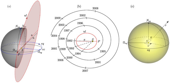
Figure 1.
General characteristics of Ulysses trajectory: (a) the relative position of the ecliptic plane ec, the solar equator plane eq, and the Ulysses orbit ul; (b) the position of the Ulysses spacecraft in orbit as a function of time; and (c) the spherical heliocentric equatorial coordinate system used in this work.
Figure 1a shows the relative position of the Sun (), the plane of the ecliptic (shown by a circle ), and the orbit of Ulysses (). The point is the north pole of the ecliptic coordinate system. The direction of Ulysses orbit is indicated by the arrow. The plane intersects the plane of the ecliptic in a straight line at an angle of 79.1°. The point is the intersection point of the Ulysses orbit with the ecliptic plane (the ascending node of the Ulysses orbit on the ecliptic). The major axis (straight line ) of the spacecraft’s orbit passes through the points: (the perihelion of the orbit) and , forming an angle of –1.1° with the line of nodes . The plane of the solar equator intersects with the plane of the ecliptic in a straight line (the line of the equator nodes on the ecliptic) at an angle of 7.25°. The point is the Northern pole of the equatorial coordinate system. The direction of the Sun’s rotation is indicated by an arrow. The angle between the node lines of the Ulysses orbit and the equator is 98.3°.
Figure 1b shows the orbit of Ulysses (ul), the perihelion of the orbit (P), and the Sun (). The time axis is shown as a spiral. To determine the position of the spacecraft in orbit at a given time, one needs to connect the mark of time on the spiral with a point , as shown by the dashed line for the time moments in years 1992, 1993, and 1994. The intersection of this segment with the orbit gives the position of the satellite at the corresponding time moment.
Figure 1c shows the spherical heliocentric equatorial coordinates used in the article. The polar angle (co-latitude) is measured from the polar axis . We also use heliolatitude defined as . The azimuthal angle (heliolongitude) is measured from the ray (i.e., from the ascending node of the equator on the ecliptic) in the direction of the Sun’s rotation (indicated by an arrow).
2.2. The Model: Basic Assumptions and Equations
The main assumption of the model is based on the fact that SW averaged over long periods of time and over large spatial scales can be considered in some approximation as a quasi-stationary axisymmetric flow [45,54,55,59,60]. In a framework of this supposition, the following simplifications were made:
- (A1) The axes of the magnetic dipole and the symmetric quadrupole of the Sun coincide with the axis of its rotation;
- (A2) SW flow at distances is quasi-stationary and axisymmetric (where is the solar radius);
- (A3) Magnetic field is frozen into the plasma, the magnetic diffusion and viscosity are not taken into account;
- (A4) SW plasma satisfies the equation of state of a monatomic ideal gas;
- (A5) Thermodynamic processes that take place in SW plasma are adiabatic.
Let us take the center of the Sun and the axis of its rotation , respectively, as the origin () and the polar axis () of a stationary spherical coordinate system , where and are the polar and azimuthal angles, and is the distance from the origin (Figure 1c).
Assumptions (A1–A5) allow us to describe the propagation of SW in spherical coordinates by the following stationary system of equations [54,60,61]:
Here, and are the velocity and magnetic induction vectors respectively (in the spherical coordinate system); , , are the electric potential, plasma density, and pressure, respectively; and is the adiabatic index. An important role is also played by both the current density vector and temperature T associated with the plasma density and pressure by the equation of state . We used the following constants: the gravitational constant G, the Sun’s mass , Boltzmann constant , and the magnetic constant .
Due to the axial symmetry the φ-projection of the Equation (1) has the form , which means that the two-dimensional vector is parallel to the two-dimensional vector at every point in space. Therefore, the system (1–5) contains seven independent equations and is written for seven independent unknown values as , , , , , , .
Let us set the boundary conditions for the system (1–5) at the sphere of the radius . Since the boundary value of the electric potential can be obtained from , , , and , and the pressure value can be calculated from the density and temperature values, it is sufficient to set the values of , , , , , , and . The boundary distribution of the azimuthal velocity was obtained from the condition of a complete corotation of the SW up to the boundary sphere , as in our previous works [54,55]:
For variables and the boundary distributions were taken constant in the model, which is the most simple, but, nevertheless, the realistic assumption
We paid special attention to the choice of boundary conditions for variables , , , and , since we hold the opinion that the correct setting of their values at the boundary sphere can provide realistic results for numerical integration of Equations (1)–(5) within the heliosphere.
To find the boundary distributions of , , , and on the basis of Ulysses spacecraft data, let us approximate their dependence on the solar distance (in units), polar angle and time t by expressions:
where and , are the first and second Legendre polynomials (corresponding to the dipole and quadrupole components in the multipole decomposition); and are the phase and cyclic frequency, respectively, of the solar dipole-quadrupole cycle; and is the time measured in years, and is the year of the solar minimum. The numerical coefficients , , , and , as well as the cyclic frequency ( is the cycle period) should be found from comparison with Ulysses data. The required boundary conditions can be obtained by substituting in expressions (8–11).
The form of time dependencies , , , and given by Formulas (8)–(11) can be interpreted as a Fourier decomposition, in which only the longest-period harmonics are taken into account. We assume that the average value of the magnetic field induction for the solar cycle is zero, i.e., . This means that there is no zero harmonic in the decompositions (8, 9) for and . For the values and , we assume that their average per cycle distributions are symmetric (even) relative to the solar equator, so the odd zero-harmonic coefficients in expressions (10) and (11) are zero: .
Earlier in Maiewski et al. [54], in a frame of axisymmetric MHD model of the SW the estimates of asymptotic behavior of the magnetic field, velocity, temperature, and plasma density were obtained, that are generally consistent with the classical Parker model [1]:
Thus, we used these asymptotics for the estimates of the Fourier decomposition coefficients as functions of and . The dependence on is modeled by the main asymptotic term: , for , , respectively. On the other hand, for radial velocity the Parker model [1] gives a logarithmic growth, but the Parker model is isothermal and our model is adiabatic. The asymptotics , for the radial velocity and temperature correspond to the adiabatic model [54,60]. Furthermore, all the asymptotics assumed by expressions (8–11) are based on our previous results [45,54,55] and correspond precisely to numerical calculations in the space domain .
The dependence , on is represented by the Legendre polynomial decomposition (multipoles), from which only the first two terms are taken into account. The dependencies , on are represented by a power series decomposition up to the second order.
Ulysses data , , , and are taken from the official website [62] and are averaged over the time interval of 25.6 days = 0.07 years, which corresponds to the sidereal period of the Sun’s rotation for the middle latitudes. The averaging over the rotation of the Sun eliminates the dependence of the solar data on the solar longitude which enables the most adequate comparison with the axisymmetric model. The averaging scheme discussed above does not take into account the angular velocity of the spacecraft, which is negligible compared to the angular velocity of the Sun.
3. Results
3.1. The Initial Data on the Boundary Sphere
The search of coefficients in decompositions (8–11) has been performed in two stages. At the first stage, the solar cycle period years and coefficients were found by the least squares method from a comparison with the Ulysses data. At the second stage, the obtained decompositions (8–11) at were used as the boundary conditions for the system (1–5), and then the numerically obtained solution was once again compared with the Ulysses data. This comparison allowed us to correct boundary conditions and finally to present them in the following form:
where is the phase shift.
The time dependence in (13) is consistent with the commonly accepted view that the radial magnetic field has a dipole shape at the minimum of the solar activity (), and a quadrupole shape at its maximum () [55,60]. Thus, we can approximately assume that during the solar 19.3-year cycle, the radial magnetic field changes according to the harmonic law (13), evolving from the dipole phase to the quadrupole one, then to the dipole with the opposite sign, and then again to the quadrupole with the opposite sign, etc.
Note that in contrast to the Formula (13), the ratio of the contributions of dipole and quadrupole components to the total expression for remains constant in (14) and during the cycle only the total amplitude factor experiences changes.
The ratio of the maximum amplitudes of the dipole and quadrupole components for and in (13, 14) remains the same and is equal to 4.5.
3.2. Comparison of Numerical Results with the Observational Data
System (1–5) with the boundary conditions (6, 7, 13–16) was solved numerically. The results were obtained for variables , , , , and calculated at discrete time moments as functions on heliodistance and polar angle . After that the numerical results were compared with similar observed data along the Ulysses trajectory, which is defined by the dependences and .
Figure 2 shows the simulation results (red line) in comparison with satellite measurements (black line) for: (a) radial velocity , (b) radial magnetic field , (c) azimuthal magnetic field , (d) temperature , and (e) density as functions on the time along the Ulysses orbit. In figures (f) and (g), the latitude and the heliodistance are correspondingly coordinates of the current position of Ulysses. Each point of the black line was obtained as a result of Ulysses measurements [62] averaged over the solar rotation period of 25.6 days. During this time, Ulysses made about measurements. Thus, each point of the black line is the averaging of the sample of the specified volume, while the vertical gray segments show the value of the standard deviation. Note that the considered dependencies cover the wide range of the heliodistance , which varies from 300 to 1150 due to the significant eccentricity (~0.6) of the Ulysses’ orbit.
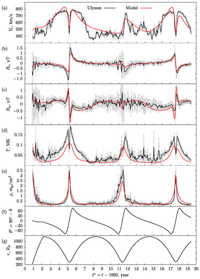
Figure 2.
Time scan of simulation results (red line) in comparison with the Ulysses data (black line): (a) radial velocity, (b) radial magnetic field, (c) azimuthal magnetic field, (d) temperature, (e) density, and (f,g) latitude and heliodistance of the current Ulysses position. Each point of the black line is the result of averaging for 25.6 days ( measurements), with half of the standard deviation () showing as a gray vertical line segment. The zero of time axis corresponds to 1990 year.
Comparison of the behavior of values in Figure 2a–e demonstrates the best agreement for radial and azimuthal magnetic components , in Figure 2b,c, as well as for plasma density in Figure 2e. Three plasma density peaks seen in Figure 2e can be associated not only with the fact that at these moments the spacecraft is near the solar equator and crosses the HCS, but also with the fact that it passes the perihelion of its orbit and is at the minimum distance from the Sun (the density of the SW plasma behaves approximately as according to the Formula (12).
It can be seen that model values of the radial plasma velocity in Figure 2a generally repeat the experimental curve and these values are comparable in order of magnitude to the experimental ones. The greatest discrepancies are evident during the years of maximum solar activity, when the role of non-stationary processes in the SW (which are not taken into account) increases.
As for the temperature profile comparisons in Figure 2d, it is obvious that the model curve, firstly, gives underestimated values of temperature and, secondly, does not describe sharp dips of its value during the passage of the HCS by spacecraft, especially noticeable during the solar minimum. The possible underestimation of the temperature values may be due to two factors: (1) in the model, the temperature decreases in the radial direction somewhat faster than in the in situ conditions; and (2) the model does not take into account non-stationary processes such as turbulence, plasma reconnection, acceleration, and heating in both HPS and HCS regions that take place in the real system [63,64].
A sharp drop in temperature value (almost two times, in HCS region during periods of solar minimum) may be associated with the properties of plasma sources near the HCS, as well as, possibly, with the interaction of plasma flows with a rarefied dust component or with other possible factors not taken into account that require further investigation and interpretation (e.g., [65,66,67,68,69]).
On the basis of this comparison, we can conclude that the model and experimental data are in a reasonable quantitative and qualitative agreement, in a framework of simplified assumptions made in the model about the quasi-stationarity of plasma processes and the absence of additional sources of heating and dissipation of plasma temperature inside the HCS.
3.3. Description of the Solar Wind Structures in the Framework of an Axisymmetric Model
The boundary conditions at the inner sphere of this model were actually determined based on the analysis of one-dimensional data measured by the Ulysses spacecraft along the trajectory of its motion. At the same time, the developed model allows us to obtain results in the form of a two-dimensional spatial distribution of physical quantities that depend on the phase of the solar cycle, and, consequently, on discrete moments of time associated with phase changes. Comparison with the Ulysses data (Figure 2) showed that the model is generally consistent with the spacecraft data. The maximum divergences are found during the years of maximum solar activity, when the contribution of non-stationary processes to the SW properties can become decisive. Thus, the model can be applied to describe the quasi-stationary averaged state of the plasma and the IMF in the heliosphere.
Below, we consider the applicability of the model to describe the general characteristics of the SW and their distribution for two characteristic periods when the relative contribution of the quadrupole component is negligible or comparable to the contribution of the dipole component. We will choose the phase of the solar cycle corresponding to the minimum solar activity in 1986 before the launch of Ulysses as a starting point (). The full cycle of the Sun’s activity is comparable to the phase shift of . Thus, the first reversal of the Sun’s magnetic field from the beginning of the reference phase takes place for the phase , while the return to the original configuration is realized for . Thus, the phases occur in the moments of maximum solar activity, when the magnetic field of the Sun is closest to a purely quadrupole configuration.
The amplitudes of the dipole and quadrupole parts in the decomposition (13) of the radial field are and , respectively. At the phase close to 0, the dipole part is negligible compared to the quadrupole. The phase is exactly in the middle in time between a pure dipole and a pure quadrupole. However, the amplitude of the dipole refers to the amplitude of the quadrupole as 4.6, so the influence of the quadrupole is still small here. Their amplitudes become equal when , i.e., at . That is, the quadrupole begins to make a significant contribution to the overall picture of the radial field at the phase , and the phase already corresponds to a pure quadrupole. We believe that in the mixed phase the picture is more interesting than in the pure phase .
Figure 3 shows the following general characteristics of the SW as functions of the heliodistance and latitude : the radial and azimuthal magnetic components , , radial velocity , temperature , and plasma density , multiplied by their corresponding asymptotic multipliers in the form defined by (12). Due to asymptotic multipliers, the plasma and magnetic physical quantities do not depend on the heliodistance (for large heliodistance values) and can be easily compared.
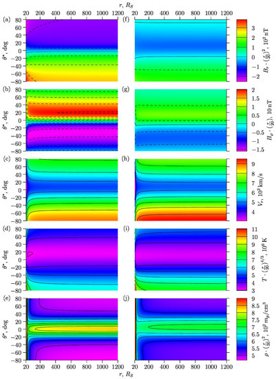
Figure 3.
According to the model: dependencies of (a,f), (b,g), (c,h), (d,i), and (e,j) on the heliodistance (in solar radii ) and latitude . All values are multiplied by their asymptotic factors (12) in the form . Figures (a,b,c,d,e) at the left panel corresponds to the phase of the cycle, figures (f,g,h,i,j) at the right one corresponds to . The lines of the zero magnetic components are marked by solid lines in figures (a,b,f,g); here the dashed lines are the remaining level lines.
Figure 3a–e at the left panel correspond to the phase , and Figure 3f–j at the right panel correspond to . In Figure 3a,b,f,g the solid lines represent the lines of zero magnetic component level, i.e., they actually indicate the position of the neutral surface of the magnetic field in the SW. The non-zero level lines in Figure 3a,b,f,g are shown as a dashed lines; in the remaining Figure 3, all level lines are shown by solid lines. At the left panel (with ) the magnetic field is almost dipole, so the position of the neutral line in the SW is almost equatorial (Figure 3a,b). The right panel (with ) corresponds to the substantial quadrupole contribution. We can see in Figure 3f that a second neutral line appeared in the Northern subpolar region, but, despite this, the subequatorial neutral line still remains almost at the equator.
It is seen in Figure 3 that at large heliodistance values the level lines become almost horizontal, which means that the physical quantities reach their asymptotic behavior (12). One can see that this happens at distances , i.e., beyond the Earth’s orbit. At the same time, some of the variables reach their horizontal asymptotics faster, while others are slower, and these trends vary slightly with the phase of the cycle.
In particular for Figure 3a,b,f,g, this means that at a fixed time moment , the neutral surfaces , in the region has approximately conic shapes with axis aligned with the axis of Sun’s rotation and the vertices pointing to its center. The angles of these cones depend on time during the cycle of solar activity. Comparison of the left and right panels in Figure 3 shows that the mixing of the dipole and quadrupole components is the reason of the formation of the magnetic field asymmetry in the Northern and Southern hemispheres. This conclusion is also consistent with other investigations [70,71].
Figure 4a–d shows the dependences at the sphere of: (a) radial magnetic field , (b) azimuthal magnetic field , (c) radial velocity , (d) temperature , and (e) density on the phase and heliolatitude . This choice of the solar distance is due to the fact that at large distances the parameters of the SW almost reach their asymptotic behavior (12), which can be seen in Figure 3. In addition, the distance approximately corresponds to the Earth’s orbit. For this distance, abundant measurements provided by various satellites are available, and the model results can be reliably compared with them.
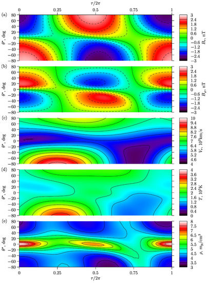
Figure 4.
According to the model: dependencies of (a), (b), (c), (d), and (e) on the cycle phase and heliolatitude at the sphere of . The solid and dashed lines mark the level lines as in Figure 3.
In Figure 4a,b, as in Figure 3a,b,f,g, solid and dashed lines represent the lines of the zero and non-zero magnetic field levels, respectively. In particular, the solid lines show the location of the neutral magnetic field surfaces. Figure 4a,b shows the evolution of the heliomagnetic field (calculated in the model) during the solar activity cycle. In the phases of maximum activity , the magnitude of the modeled magnetic field is minimum in the cycle.
The position of the neutral line in the SW separating the magnetic fluxes of the opposite polarity is of particular interest. Therefore, at the beginning of the cycle (solar minimum), the neutral line is located at the zero latitude. Then it moves to the Southern hemisphere, and another neutral line appears in the Northern hemisphere. According to model, during the time of solar activity maximum in the SW, two neutral lines can simultaneously exist at high latitudes in the Northern and Southern hemispheres. As it can be seen from Figure 4c,d, the distribution of both radial velocity and temperature in the SW has a pronounced asymmetry in the Northern and Southern hemispheres during periods of maximum solar activity. The temperature and density of the plasma in Figure 4d,e, as a whole, correlate with the position of the neutral or current surfaces, and they are in the counter-phase: the maximum density corresponds to the minimum temperature and vice versa.
It is known that at high latitudes, the radial SW velocity reaches the greater values (fast SW) than in the subequatorial region (slow SW). Our calculations show in Figure 4c that, during the solar cycle, the ratio of radial velocities at the poles can changes significantly, but in the near-equatorial region, the radial velocity remains almost constant. According to Figure 4c, the radial velocity in the Southern circumpolar region changes with a greater amplitude than in the Northern one. At the same time, the maximum of the radial velocity at the North is achieved approximately during the dipole phase of the cycle, while the maximum of at the South occurs at the quadrupole phase.
Let us consider the behavior of the temperature as a function on latitude in Figure 4d. Generally, the temperature distribution is similar to the radial velocity distribution. Thus, in the circumpolar regions, the temperature is usually higher than in the subequatorial region. However, the relationship is more complex than for the radial velocity, and the temperature asymmetry of hemispheres is more pronounced. At different phases of the cycle, the dependence of temperature on latitude is different. In the dipole phase, a noticeable maximum appears at the equator. In the quadrupole phase, it is absent. In some transition phases, the north-south asymmetry is so large that the dependence becomes monotonic.
Concerning the density , during almost all phases of the cycle it reaches its maximum near the equator and minimum in the circumpolar regions (Figure 4e). This maximum is pronounced in the dipole phase more than in the quadrupole phase. Moreover, during the transition from the dipole phase to the quadrupole phase, the maximum density shifts from the equator, following the evolution of the neutral line , but the second maximum does not appear. In the second quadrupole phase (), the maximum is so weakly expressed that the dependence becomes almost monotonous.
3.4. Geometry of Neutral Surfaces in the Solar Wind
Let us consider in more detail the question of the geometry of the magnetic neutral surfaces in the SW. From the comparison of the dependence of the modeling radial magnetic component with latitude of spacecraft in orbit shown in Figure 2b,f, it can be seen that the radial magnetic field is approximately dipole over the entire period of time except for 2001–2002. This is shown more clearly in Figure 5.
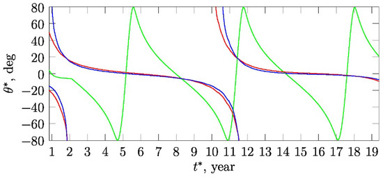
Figure 5.
According to the model: cross-section of neutral surfaces (red line) and (blue line) of the Ulysses trajectory (green line). For each moment of the time, the corresponding points on the red and blue lines indicate the position ( coordinate) of neutral lines at the sphere , which corresponds to the local position of spacecraft. The zero of time axis corresponds to 1990 year.
Let us have a look at the neutral surfaces in Figure 5. One can see that for a significant part of the cycle, there is a single such surface (i.e., single value of ), inclined to the equator by no more than .
In quite short periods of time (May 1990–1992 and 2000–May 2001), according to the model, there are two neutral surfaces. The durations of these time intervals are 6.9% of the cycle period, i.e., 1.33 years (as it mentioned above the cycle period is 19.3 years—according to the model). The radial field is mostly quadrupole during this interval. According to the model, in 2001, the satellite crossed the neutral surface two times. Therefore, during this time interval, Ulysses observes mostly quadrupole radial magnetic field . Comparison with Figure 2b shows that the measured changes of the radial field were more complicated during this interval, sometimes being in counter-phase with the model data. However, the red line of the model data in Figure 2b confidently fits between the gray bars of the root-mean-square errors, which are very large during this interval.
The current density is defined by , therefore, the radial magnetic field is related with the azimuthal current , and azimuthal field is related with radial current . In our previous works [45,54,55], it was shown that on the sphere with heliodistance the azimuthal current is maximum when approximately , i.e., the neutral surface corresponds to current sheet . Analogically, the maximum of a radial current is concentrated on a neutral surface . Let us note that accordingly to Figure 5, the deviation of the neutral surfaces and from the equatorial plane is not large and generally does not exceed .
4. Discussion
In this paper, we present a model that allows us to determine the parameters of the SW along the orbit of the Ulysses spacecraft. A quasi-stationary axisymmetric self-consistent MHD model was constructed to simulate the SW observations. The model permits the finding of the spatial distribution of the characteristics of the magnetic field and plasma at distances from 20 to 1200 Solar radii at almost all solar latitudes. A comparison of the characteristics of the magnetic and plasma data of Ulysses spacecraft during its flight in the heliosphere from 1990 to 2009 years with simulation results obtained in the framework of our stationary axisymmetric MHD model of SW is performed. As a development of idea by Kim et al. [53], the averaging used in our model allowed us to study large scale distribution of SW characteristics for different latitudes and heliocentric distances in the interplanetary space. The model also takes into account the mutual influence of the IMF and the plasma velocity field.
The peculiarity of this model is that the non-adiabatic and non-stationary processes occuring in the SW are not taken into account. Really these processes can be accompanied by plasma heating/acceleration or temperature depressions [13,72,73]. SW can be heated locally by interacting with propagating waves [74] as well as with shock waves of planetary magnetospheres, or CME (coronal mass ejections) or CIR (corotating interaction regions) (e.g., [75,76,77,78]). Turbulence and magnetic reconnection processes are assumed to be the main mechanisms of plasma heating ([13], and references therein).
The absence of accounting for heating processes can lead to the underestimation of plasma temperature in the SW during periods of maximum solar activity, when the role of non-stationary and non-adiabatic processes increases (Figure 2d). In some SW models, the heating on turbulence was taken into account [48,79,80]. It was shown in works [81,82,83,84] that the effects of turbulent cascade influence the SW temperature and its evolution. In our model, only most general characteristics of the SW were considered, in particular, the processes of formation and evolution of large-scale current sheets, along with the HCS. Non-adiabatic processes were not taken into account.
As it follows from the comparison of theoretical and experimental data along the Ulysses trajectory in Figure 2, the description of the magnetic field in the model is in satisfactory agreement with the observational data; thus, the model results mostly lie within the corridor of standard deviations. Large-scale changes of IMF in the SW, depending on the solar cycle, are, at best, consistent with model results during the minimum periods. General discrepancies are observed during periods of solar maxima, when the heliomagnetic field is dominated by the quadrupole component, and the model predicts the presence of two neutral surfaces at high latitudes instead of one neutral surface in the subequatorial region at the minimum. Thus, the Ulysses data show the intersection of several current sheets (at least three zero-value intersections are visible) in the subequatorial region during the years near the maxima of solar activity. This may be due to the presence of not only quadrupole magnetic component of the heliomagnetic field, but also the octupole component, which is not taken into account in our model. A possible geometry of large-scale current sheets in SW, taking into account the octupole component, is given in [59,85], where it is shown that, under its presence, the appearance of three neutral lines are characteristic for the SW, i.e., one of them is located at low latitudes and the other two are located at high latitudes.
Large-scale changes of the SW radial velocity are roughly consistent with the model data, although it is obvious that the model does not describe small-scale fluctuations. Comparison of plasma density shows a quite good agreement between observational data and numerical calculations.
The largest deviations of the model results from the Ulysses data are noticeable on temperature profiles, where the model gives underestimated (~1.5–2 times) temperature values. In addition, Ulysses observations show a sharp temperature dips in the HCS/HPS region. The general underestimation of the value of plasma temperature in the SW may be due to the fact that the model does not take into account the processes of plasma heating in the solar corona (flares, coronal mass ejections, etc.), as well as the local non-stationary processes. The problem of underestimating of theoretical dependences in comparison with the observational data is the important problem that requires the identification of additional energy sources in the SW that can contribute to the local or global heating of the plasma inside the HPS. As for the sharp temperature dips inside the HPS, as mentioned above, they may be due to the influence of slow-wave sources, as well as the dust component of the plasma in the heliospheric current sheet, or other reasons [6,7,22,67,68,69,86].
In this paper, we compared, for the first time, the results of the MHD model of the SW with 25.6 day averages of SW observations by Ulysses spacecraft along its trajectory at low and high latitudes, at different radial distances from the Sun and in different phases of the solar cycle. A satisfactory agreement was obtained in the description of large-scale changes of IMF, plasma density, and radial velocity in SW, which indicates the adequacy of the model and the possibility of its applicability for similar studies in other areas of the heliosphere. At the same time, it is shown that the setting of adequate boundary conditions on the sphere around the Sun, taken with the same order of SW parameters from experimental observations, gives the underestimated temperature of SW plasma at low latitudes and does not explain the features of radial plasma temperature profiles in the subequatorial region. This suggests the necessity to take into account some additional heating factors in the model, both global (e.g., processes in the solar corona) and local (e.g., turbulence [87], shock waves [88], and magnetic reconnection in SW [13]).
In conclusion, we note that the results of recently launched spacecraft Solar Orbiter would be very interesting and useful for space research, particularly for presented theoretical work, because Solar Orbiter should observe the Sun’s polar regions and answer the general question “How does the Sun create and control the heliosphere?” [89]. We suppose that new observational data allow solving the questions of the evolution and displacement of the HCS in the solar activity cycle, as well as the question of possible existence of several large-scale current sheets in the heliosphere, that are the objects of our theoretical consideration. Perhaps the obtained data make it possible to draw a global current circuit linking together the entire heliosphere from the corona of the Sun to the heliopause, investigate its evolution in the solar cycle, and to understand its driver.
Author Contributions
Conceptualization, L.M.Z. and H.V.M.; methodology, H.V.M. and E.V.M.; software, E.V.M.; validation, E.V.M. and V.Y.P.; formal analysis, E.V.M., H.V.M. and V.Y.P.; investigation, E.V.M., H.V.M. and V.Y.P.; resources, E.V.M. and V.Y.P.; data curation, E.V.M.; writing—original draft preparation, E.V.M., H.V.M. and V.Y.P.; writing—review and editing, L.M.Z. and H.V.M.; visualization, E.V.M.; supervision, L.M.Z.; project administration, L.M.Z.; funding acquisition, L.M.Z. and H.V.M. All authors have read and agreed to the published version of the manuscript.
Funding
This research received no external funding.
Informed Consent Statement
Not applicable.
Data Availability Statement
Not applicable.
Acknowledgments
Authors acknowledge O.V. Khabarova and R.A. Kislov for fruitful discussions and valuable comments. This research was partially supported through computational resources of HPC facilities at HSE University.
Conflicts of Interest
The authors declare no conflict of interest.
References
- Parker, E.N. Dynamics of the interplanetary gas and magnetic fields. Astrophys. J. 1958, 128, 664. [Google Scholar] [CrossRef]
- Bondi, H. On spherically symmetric accretion. MNRAS 1952, 112, 195. [Google Scholar] [CrossRef]
- Neugebauer, M.; Snyder, C.W. Mariner 2 Observations of the Solar Wind, 2, Relation of Plasma Properties to the Magnetic Field. J. Geophys. Res. 1967, 72, 1823. [Google Scholar] [CrossRef]
- Veselovsky, I.S. Magnetic Domains in the Heliosphere During Solar Maximum Years. Space Sci. Rev. 2001, 97, 109–112. [Google Scholar] [CrossRef]
- Abbo, L.; Ofman, L.; Antiochos, S.K.; Hansteen, V.H.; Harra, L.; Ko, Y.-K.; Lapenta, G.; Li, B.; Riley, P.; Strachan, L.; et al. Slow Solar Wind: Observations and Modeling. Space Sci. Rev. 2016, 201, 55–108. [Google Scholar] [CrossRef]
- Bruno, R.; Carbone, V. The Solar Wind as a Turbulence Laboratory. Living Rev. Sol. Phys. 2013, 10, 2. [Google Scholar] [CrossRef]
- Matthaeus, W.H.; Velli, M. Who Needs Turbulence? Space Sci. Rev. 2011, 160, 145–168. [Google Scholar] [CrossRef]
- Wang, S.; Liu, Y.F.; Zheng, H.N. Magnetic reconnection in multiple heliospheric current sheets. Sol. Phys. 1997, 173, 409–426. [Google Scholar] [CrossRef]
- Balogh, A.; Erdõs, G. The Heliospheric Magnetic Field. Space Sci. Rev. 2013, 176, 177–215. [Google Scholar] [CrossRef]
- Hoeksema, J.T. The Large-Scale Structure of the Heliospheric Current Sheet during the ULYSSES Epoch. Space Sci. Rev. 1995, 72, 137. [Google Scholar] [CrossRef]
- Khabarova, O.; Zank, G.P.; Li, G.; Le Roux, J.A.; Webb, G.M.; Dosch, A.; Malandraki, O.E. Small-scale Magnetic Islands in the Solar Wind and Their Role in Particle Acceleration. I. Dynamics of Magnetic Islands Near the Heliospheric Current Sheet. Astrophys. J. 2015, 808, 181. [Google Scholar] [CrossRef]
- Khabarova, O.V.; Zank, G.P.; Li, G.; Malandraki, O.E.; Le Roux, J.A.; Webb, G.M. Small-scale Magnetic Islands in the Solar Wind and Their Role in Particle Acceleration. II. Particle Energization inside Magnetically Confined Cavities. Astrophys. J. 2016, 827, 122. [Google Scholar] [CrossRef]
- Malandraki, O.E.; Khabarova, O.V.; Bruno, R.; Zank, G.P.; Li, G.; Jackson, B.; Bisi, M.M.; Greco, A.; Pezzi, O.; Matthaeus, W.; et al. Current Sheets, Magnetic Islands, and Associated Particle Acceleration in the Solar Wind as Observed by Ulysses near the Ecliptic Plane. Astrophys. J. 2019, 881, 116. [Google Scholar] [CrossRef]
- Gary, S.P. Microinstabilities upstream of the earth’s bow shock: A brief review. J. Geophys. Res. 1981, 86, 4331–4336. [Google Scholar] [CrossRef]
- Kasper, J.C.; Lazarus, A.J.; Gary, S.P. Wind/SWE observations of firehose constraint on solar wind proton temperature anisotropy. Geophys. Res. Lett. 2002, 29, 20-1–20-4. [Google Scholar] [CrossRef]
- Klein, K.G.; Alterman, B.L.; Stevens, M.L.; Vech, D.; Kasper, J.C. Majority of Solar Wind Intervals Support Ion-Driven Instabilities. Phys. Rev. Lett. 2018, 120, 205102. [Google Scholar] [CrossRef]
- Maruca, B.A.; Chasapis, A.; Gary, S.P.; Bandyopadhyay, R.; Chhiber, R.; Parashar, T.N.; Matthaeus, W.H.; Shay, M.A.; Burch, J.L.; Moore, T.E.; et al. MMS Observations of Beta-dependent Constraints on Ion Temperature Anisotropy in Earth’s Magnetosheath. Astrophys. J. 2018, 866, 25. [Google Scholar] [CrossRef]
- Alfven, H. Electric currents in cosmic plasmas. Rev. Geophys. S Phys. 1977, 15, 27. [Google Scholar] [CrossRef]
- Israelevich, P.L.; Gombosi, T.I.; Ershkovich, A.I.; Hansen, K.C.; Groth, C.P.T.; DeZeeuw, D.L.; Powell, K.G. MHD simulation of the three-dimensional structure of the heliospheric current sheet. Astron. Astrophys. 2001, 376, 288–291. [Google Scholar] [CrossRef]
- Richardson, J.D.; Burlaga, L.F. The Solar Wind in the Outer Heliosphere and Heliosheath. Space Sci. Rev. 2013, 176, 217–235. [Google Scholar] [CrossRef]
- Pogorelov, N.V.; Fichtner, H.; Czechowski, A.; Lazarian, A.; Lembege, B.; le Roux, J.A.; Potgieter, M.S.; Scherer, K.; Stone, E.C.; Strauss, R.D.; et al. Heliosheath Processes and the Structure of the Heliopause: Modeling Energetic Particles, Cosmic Rays, and Magnetic Fields. Space Sci. Rev. 2017, 212, 193–248. [Google Scholar] [CrossRef]
- Lacombe, C.; Salem, C.; Mangeney, A.; Steinberg, J.-L.; Maksimovic, M.; Bosqued, J.M. Latitudinal distribution of the solar wind properties in the low- and high-pressure regimes: Wind observations. Ann. Geophys. 2000, 18, 852–865. [Google Scholar] [CrossRef]
- Eselevich, E.G.; Fainshtein, V.G.; Rudenko, G.V. Study of the structure of streamer belts and chains in the solar corona. Sol. Phys. 1999, 188, 277. [Google Scholar] [CrossRef]
- Crooker, N.U.; Kahler, S.W.; Larson, D.E.; Lin, R.P. Large-scale magnetic field inversions at sector boundaries. J. Geophys. Res. 2004, 109, A03108. [Google Scholar] [CrossRef]
- Winterhalter, D.; Smith, E.J.; Burton, M.E.; Murphy, N.; McComas, D. The heliospheric plasma sheet. J. Geophys. Res. 1994, 99, 6667–6680. [Google Scholar] [CrossRef]
- Büchner, J.; Zelenyi, L.M. Regular and chaotic charged particle motion in magnetotaillike field reversals: 1. Basic theory of trapped motion. J. Geophys. Res. 1989, 94, 11821. [Google Scholar] [CrossRef]
- Malova, H.V.; Popov, V.Y.; Grigorenko, E.E.; Petrukovich, A.A.; Delcourt, D.; Sharma, A.S.; Khabarova, O.V.; Zelenyi, L.M. Evidence for quasi-adiabatic motion of charged particles in strong current sheets in the solar wind. Astrophys. J. 2017, 834, 34. [Google Scholar] [CrossRef]
- Malova, K.V.; Popov, V.Y.; Khabarova, O.V.; Grigorenko, E.E.; Petrukovich, A.A.; Zelenyi, L.M. Structure of Current Sheets with Quasi-Adiabatic Dynamics of Particles in the Solar Wind. Cos. Res. 2018, 56, 445. [Google Scholar] [CrossRef]
- Mursula, K.; Hiltula, T. Systematically asymmetric heliospheric magnetic field: Evidence for a quadrupole mode and non-axisymmetry with polarity flip-flops. Sol. Phys. 2004, 224, 133–143. [Google Scholar] [CrossRef]
- Wilcox, J.M.; Hoeksema, J.T.; Scherrer, P.H. Origin of the warped heliospheric current sheet. Science 1980, 209, 603. [Google Scholar] [CrossRef]
- Echer, E.; Bolzan, M.J.A.; Franco, A.M.S. Statistical analysis of solar wind parameter variation with heliospheric distance: Ulysses observations in the ecliptic plane. Adv. Space Res. 2020, 65, 2846. [Google Scholar] [CrossRef]
- Reisenfeld, D.B.; Wiens, R.C.; Barraclough, B.L.; Steinberg, J.T.; Neugebauer, M.; Raines, J.; Zurbuchen, T.H. Solar Wind Conditions and Composition during the Genesis Mission as Measured by In Situ Spacecraft. Space Sci. Rev. 2013, 175, 125. [Google Scholar] [CrossRef]
- Tokumaru, M.; Fujiki, K.; Iju, T. North-south asymmetry in global distribution of the solar wind speed during 1985–2013. J. Geophys. Res. 2015, 120, 3283. [Google Scholar] [CrossRef]
- Vsekhsvyatskiy, S.K. The Solar Wind and Solar Corpuscular Streams. Geomagn. Aeron. 1964, 4, 255. [Google Scholar]
- Parker, E.N. Dynamical Theory of the Solar Wind. Space Sci. Rev. 1965, 4, 666. [Google Scholar] [CrossRef]
- Gringauz, K.I.; Bezrokikh, V.V.; Ozerov, V.D.; Rybchinskii, R.E. A Study of the Interplanetary Ionized Gas, High-Energy Electrons and Corpuscular Radiation from the Sun by Means of the Three-Electrode Trap for Charged Particles on the Second Soviet Cosmic Rocket. Sov. Phys. Dokl. 1960, 5, 361. [Google Scholar]
- Gringauz, K.I.; Zastenker, G.N.; Khokhlov, M.Z. Velocity and temperature of the solar wind from data of the interplanetary station Venus 3. Kosm. Issled. 1970, 8, 948–951. [Google Scholar]
- Schatten, K.H.; Wilcox, J.M.; Ness, N.F. A model of interplanetary and coronal magnetic fields. Sol. Phys. 1969, 6, 442–455. [Google Scholar] [CrossRef]
- Schatten, K.H. Current Sheet Magnetic Model for the Solar Corona. Cosm. Electrodyn. 1971, 2, 232–245. [Google Scholar]
- Arge, C.N.; Pizzo, V.J. Improvement in the prediction of solar wind conditions using near-real time solar magnetic field updates. J. Geophys. Res. 2000, 105, 10465–10480. [Google Scholar] [CrossRef]
- Levine, R.H.; Schulz, M.; Frazier, E.N. Simulation of the magnetic structure of the inner heliosphere by means of a non-spherical source surface. Sol. Phys. 1982, 77, 363–392. [Google Scholar] [CrossRef]
- Schultz, M.; Frazier, E.N.; Boucher, D.J. Coronal magnetic-field model with non-spherical source surface. Sol. Phys. 1978, 60, 83. [Google Scholar] [CrossRef]
- Wang, Y.M.; Young, P.R.; Muglach, K. Evidence for two separate heliospheric current sheets of cylindrical shape during Mid-2012. Astrophys. J. 2014, 780, 103. [Google Scholar] [CrossRef]
- Schultz, M. Conical Current Sheets in a Source-Surface Model of the Heliosphere. AGU Fall Meeting Abstracts, SAO/NASA Astrophysics Data System. 2007, SH53A-1069. Available online: https://ui.adsabs.harvard.edu/abs/2007AGUFMSH53A1069S (accessed on 10 April 2022).
- Maiewski, E.V.; Malova, H.V.; Kislov, R.A.; Popov, V.Y.; Petrukovich, A.A.; Khabarova, O.V.; Zelenyi, L.M. Formation of Multiple Current Sheets in the Heliospheric Plasma Sheet. Cosm. Res. 2020, 58, 411–425. [Google Scholar] [CrossRef]
- Gombosi, T.I.; van der Holst, B.; Manchester, W.B.; Sokolov, I.V. Extended MHD modeling of the steady solar corona and the solar wind. Living Rev. Sol. Phys. 2018, 15, 4. [Google Scholar] [CrossRef]
- Riley, P.; Linker, J.A.; Mikić, Z. Modeling the heliospheric current sheet: Solar cycle variations. J. Geophys. Res. 2002, 107, SSH 8-1–SSH 8-6. [Google Scholar] [CrossRef]
- Usmanov, A.V.; Matthaeus, W.H.; Goldstein, M.L.; Chhiber, R. The Steady Global Corona and Solar Wind: A Three-dimensional MHD Simulation with Turbulence Transport and Heating. Astrophys. J. 2018, 865, 25. [Google Scholar] [CrossRef]
- van der Holst, B.; Huang, J.; Sachdeva, N.; Kasper, J.C.; Manchester, W.B.; Borovikov, D.; Chandran, B.D.G.; Case, A.W.; Korreck, K.E.; Larson, D.; et al. Improving the Alfvén Wave Solar Atmosphere Model Based on Parker Solar Probe Data. Astrophys. J. 2022, 925, 146. [Google Scholar] [CrossRef]
- Neugebauer, M.; Forthyth, R.J.; Galvin, A.B.; Harvey, K.L.; Hoeksema, J.T.; Lazarus, A.J.; Lepping, R.P.; Linker, J.A.; Mikic, Z.; Steinberg, J.T.; et al. Spatial structure of the solar wind and comparisons with solar data and models. J. Geophys. Res. 1998, 103, 14587. [Google Scholar] [CrossRef]
- Georgieva, K. Space weather and space climate—What the look from the earth tells us about the sun. In The Environments of the Sun and the Stars; Rozelot, J.-P., Neiner, C., Eds.; Springer: Berlin, Germany, 2013; pp. 53–107. [Google Scholar]
- Usmanov, A.V. A Global Numerical Three-Dimensional Magnetohydrodynamic Model of the Solar Wind. Sol. Phys. 1993, 146, 377–396. [Google Scholar] [CrossRef]
- Kim, T.K.; Pogorelov, N.V.; Zank, G.P.; Elliott, H.A.; McComas, D.J. Modeling the Solar Wind at the Ulysses, Voyager and New Horizons Spacecraft. Astrophys. J. 2016, 832, 72. [Google Scholar] [CrossRef]
- Maiewski, E.V.; Kislov, R.A.; Malova, H.V.; Popov, V.Y.; Petrukovich, A.A. Model of Solar Wind in the Heliosphere at Low and High Latitudes. Plasma Phys. Rep. 2018, 44, 80–91. [Google Scholar] [CrossRef]
- Maiewski, E.V.; Kislov, R.A.; Khabarova, O.V.; Malova, H.V.; Popov, V.Y.; Petrukovich, A.A.; Zelenyi, L.M. Magnetohydrodynamic modeling of the solar wind key parameters and current sheets in the heliosphere: Radial and solar cycle evolution. Astrophys. J. 2020, 892, 12. [Google Scholar] [CrossRef]
- Pneuman, G.W.; Kopp, R.A. Gas-Magnetic Field Interactions in the Solar Corona. Sol. Phys. 1971, 18, 258–270. [Google Scholar] [CrossRef]
- Marsden, R.G. (Ed.) The High Latitude Heliosphere; Kluwer Academic Publishers: Dordrecht, The Netherlands, 1995; ISBN 0-7923-3229-6. [Google Scholar]
- Dmitriev, A.V.; Suvorova, A.V.; Veselovsky, I.S.; Zeldovich, M.A. Coronal Imprints in the Heliospheric Plasma and Magnetic Fields at the Earth’s Orbit during the Last Three Solar Minima. Adv. Space Res. 2000, 25, 1965–1968. [Google Scholar] [CrossRef]
- Usmanov, A.V. Interplanetary magnetic field structure and solar wind parameters as inferred from solar magnetic field observations and by using a numerical 2-D MHD model. Sol. Phys. 1993, 143, 345–363. [Google Scholar] [CrossRef]
- Kislov, R.A.; Khabarova, O.V.; Malova, H.V. Quasi-stationary Current Sheets of the Solar Origin in the Heliosphere. Astrophys. J. 2019, 875, 28. [Google Scholar] [CrossRef]
- Priest, E. Magnetohydrodynamics of the Sun, 2nd ed.; Cambridge University Press: Cambridge, UK, 2014. [Google Scholar] [CrossRef]
- Ulysses Final Archive. The Directory VHM_FGM Contains the Ulysses Prime Resolution Data of the Magnetic Field, Directory SWOOPS Presents Plasma Speed, Density and Temperature Data. Available online: http://ufa.esac.esa.int/ufa/#data (accessed on 13 April 2022).
- Lee, M.A.; Mewaldt, R.A.; Giacalone, J. Shock Acceleration of Ions in the Heliosphere. Space Sci. Rev. 2012, 173, 247–281. [Google Scholar] [CrossRef]
- Cranmer, S.R.; Gibson, S.E.; Riley, P. Origins of the Ambient Solar Wind: Implications for Space Weather. Space Sci. Rev. 2017, 212, 1345. [Google Scholar] [CrossRef]
- Poppe, A.R.; Lee, C.O. The Effects of Solar Wind Structure on Nanodust Dynamics in the Inner Heliosphere. J. Geophys. Res. 2020, 125, e28463. [Google Scholar] [CrossRef]
- Yermolaev, Y.I.; Stupin, V.V. Helium abundance and dynamics in different types of solar wind streams: The Prognoz 7 observations. J. Geophys. Res. 1997, 102, 2125–2136. [Google Scholar] [CrossRef]
- Gazis, P.R.; Barnes, A.; Mihalov, J.D. Pioneer and Voyager Observations of Large-Scale Spatial and Temporal Variations in the Solar Wind. Space Sci. Rev. 1995, 72, 117–120. [Google Scholar] [CrossRef]
- Smith, E.J. The heliospheric current sheet. J. Geophys. Res. 2001, 106, 15819–15832. [Google Scholar] [CrossRef]
- Burlaga, L.F.; Ness, N.F.; Wang, Y.-M.; Sheeley, N.R. Heliospheric magnetic field strength and polarity from 1 to 81 AU during the ascending phase of solar cycle 23. J. Geophys. Res. 2002, 107, 1410. [Google Scholar] [CrossRef]
- Tsareva, O.O. Generalization of Stormer theory for an axisymmetric superposition of dipole and quadrupole fields. J. Geophys. Res. Space Phys. 2019, 124, 2844–2853. [Google Scholar] [CrossRef]
- Sokoloff, D.D.; Malova, H.V.; Yushkov, E. Symmetries of Magnetic Fields Driven by Spherical Dynamos of Exoplanets and Their Host Stars. Symmetry 2020, 12, 2085. [Google Scholar] [CrossRef]
- Richardson, I.G.; Cane, H.V. Regions of abnormally low proton temperature in the solar wind (1965–1991) and their association with ejecta. J. Geophys. Res. 1995, 100, 23397–23412. [Google Scholar] [CrossRef]
- Richardson, J.D.; Paularena, K.I.; Lazarus, A.J.; Belcher, J.W. Radial evolution of the solar wind from IMP 8 to Voyager 2. Geophys. Res. Lett. 1995, 22, 325–328. [Google Scholar] [CrossRef]
- Zhao, G.-Q.; Feng, H.-Q.; Wu, D.-J.; Liu, Q.; Zhao, Y.; Tian, Z.-J. On Mechanisms of Proton Perpendicular Heating in the Solar Wind: Test Results Based on Wind Observations. Res. Astr. Astrophys. 2022, 22, 015009. [Google Scholar] [CrossRef]
- Gloeckler, G. Observation of Injection and Pre-Acceleration Processes in the Slow Solar Wind. Space Sci. Rev. 1999, 89, 91–104. [Google Scholar] [CrossRef]
- Mewaldt, R.A.; Cohen, C.M.S.; Mason, G.M. The Source Material for Large Solar Energetic Particle Events. Geophys. Union Geophys. Monogr. Ser. 2006, 165, 115–126. [Google Scholar] [CrossRef]
- Keesee, A.M.; Elfritz, J.G.; Fok, M.-C.; McComas, D.J.; Scime, E.E. Superposed epoch analyses of ion temperatures during CME- and CIR/HSS-driven storms. J. Atmos. Sol. Terr. Phys. 2014, 115, 67–78. [Google Scholar] [CrossRef]
- Squire, J.; Meyrand, R.; Kunz, M.W.; Arzamasskiy, L.; Schekochihin, A.A.; Quataert, E. High-frequency heating of the solar wind triggered by low-frequency turbulence. Nat. Astr. 2022. [Google Scholar] [CrossRef]
- Adhikari, L.; Zank, G.P.; Zhao, L.-L. A Solar Coronal Hole and Fast Solar Wind Turbulence Model and First-orbit Parker Solar Probe (PSP) Observations. Astrophys. J. 2020, 901, 102. [Google Scholar] [CrossRef]
- Zank, G.P.; Zhao, L.-L.; Adhikari, L.; Telloni, D.; Kasper, J.C.; Bale, S.D. Turbulence transport in the solar corona: Theory, modeling, and Parker Solar Probe. Phys. Plasmas 2021, 28, 080501. [Google Scholar] [CrossRef]
- Kiyani, K.H.; Chapman, S.C.; Sahraoui, F.; Hnat, B.; Fauvarque, O.; Khotyaintsev, Y.V. Enhanced Magnetic Compressibility and Isotropic Scale Invariance at Sub-ion Larmor Scales in Solar Wind Turbulence. Astrophys. J. 2013, 763, 10. [Google Scholar] [CrossRef]
- Hadid, L.Z.; Sahraoui, F.; Galtier, S. Energy Cascade Rate in Compressible Fast and Slow Solar Wind Turbulence. Astrophys. J. 2017, 838, 9. [Google Scholar] [CrossRef]
- Bandyopadhyay, R.; Chasapis, A.; Chhiber, R.; Parashar, T.N.; Maruca, B.A.; Matthaeus, W.H.; Schwartz, S.J.; Eriksson, S.; Le Contel, O.; Breuillard, H.; et al. Solar Wind Turbulence Studies Using MMS Fast Plasma Investigation Data. Astrophys. J. 2018, 866, 81. [Google Scholar] [CrossRef]
- Qudsi, R.A.; Bandyopadhyay, R.; Maruca, B.A.; Parashar, T.N.; Matthaeus, W.H.; Chasapis, A.; Gary, S.P.; Giles, B.L.; Gershman, D.J.; Pollock, C.J.; et al. Intermittency and Ion Temperature-Anisotropy Instabilities: Simulation and Magnetosheath Observation. Astrophys. J. 2020, 895, 83. [Google Scholar] [CrossRef]
- Réville, V.; Brun, A.S.; Matt, S.P.; Strugarek, A.; Pinto, R.F. The effect of magnetic topology on thermally driven wind: Toward a general formulation of the braking law. Astrophys. J. 2015, 798, 116. [Google Scholar] [CrossRef]
- Burlaga, L.F.; Ness, N.F.; Richardson, J.D. Heliosheath magnetic field and plasma observed by Voyager 2 during 2011. J. Geophys. Res. 2014, 119, 6062–6073. [Google Scholar] [CrossRef]
- Huang, S.Y.; Zhang, J.; Yuan, Z.G.; Jiang, K.; Wei, Y.Y.; Xu, S.B.; Xiong, Q.Y.; Zhang, Z.H.; Lin, R.T.; Yu, L. Intermittent Dissipation at Kinetic Scales in the Turbulent Reconnection Outflow. Geophys. Res. Lett. 2022, 49, e2021GL096403. [Google Scholar] [CrossRef]
- Reames, D.V. Abundances, Ionization States, Temperatures, and FIP in Solar Energetic Particles. Space Sci. Rev. 2018, 214, 61. [Google Scholar] [CrossRef]
- Marirrodriga, C.G.; Pacros, A.; Strandmoe, S.; Arcioni, M.; Arts, A.; Ashcroft, C.; Ayache, L.; Bonnefous, Y.; Brahimi, N.; Cipriani, F.; et al. The Solar Orbiter: Mission and spacecraft design. Astr. Astrophys. 2021, 646, A121. [Google Scholar] [CrossRef]


Publisher’s Note: MDPI stays neutral with regard to jurisdictional claims in published maps and institutional affiliations. |
© 2022 by the authors. Licensee MDPI, Basel, Switzerland. This article is an open access article distributed under the terms and conditions of the Creative Commons Attribution (CC BY) license (https://creativecommons.org/licenses/by/4.0/).