Can Asteroid Belts Exist in the Luyten’s System?

Abstract

The extra-solar planetary system Luyten is relatively close (12.3 light years) to our Sun. The Luyten’s red dwarf star is orbited by four planets, two of them Earth-like (in mass) and in 4:1 resonance. Extra-solar systems might contain asteroid belts such as ours. Therefore, it is important to investigate whether it is possible to have a stable population of minor bodies and compare them to those in our system. The study of extra-solar systems is crucial for understanding the evolution of planetary systems in general. Here, we investigate the stability of two possible asteroid populations in the Luyten’s system: the main asteroid belt between the two inner and two outer planets, and an outer asteroid belt, situated beyond the planets. We also explore the likelihood of observing an asteroid or a dwarf planet in this system. Our study suggests that the existence of asteroid belts is possible, notably the main belt at 0.09–0.53 au from the star and an outer belt (with the inner boundary at 0.85 au and the outer boundary at ∼66,000 au). The average Yarkovsky drift for the Luyten’s main asteroid belt is ∼$0.5\times {10}^{-4}$ au/Myr for km-size objects. The Luyten’s system might host extra-solar minor bodies, some of which could be capable of entering our own system. Presently, no asteroids can be detected in the Luyten’s system, not even a Ceres-sized body, because the detection signal using the radial velocity method is at least two orders of magnitude less than that required for discerning such objects. The detection probability of an asteroid in the Luyten belt similar to Ceres is about 1.3%, which is less than the probability of finding Luyten B (∼3%).

1. Introduction

The Luyten’s planetary system, situated at a distance of ∼12.3 light years in the constellation Canis Minor, is the nearest known planetary system after Proxima Centauri (e.g., [1,2]). The central star, Luyten A (GJ 273a), is an M3.5V red dwarf (26% mass of the Sun’s [3]). Luyten A is orbited by four planets (e.g., [1,2,4]); the two inner planets, Luyten C (GJ 273c) and Luyten B (GJ 273b), have been confirmed, while the two outer planets, Luyten D (GJ 273d) and Luyten E (GJ 273e), remain promising candidates [2,4]. The inner planets orbit with a very small semi-major axis compared to our solar system planets (

Table 1. Osculating elements of Luyten C and Luyten B [1,4] and mass (in Sun masses) for all planets. The radius was computed assuming the density equivalent to that of the Earth’s ($\rho =$ 5514 kg/m${}^3$) for the inner planets and to that of Saturn’s ($\rho =$ 687 kg/m${}^3$) and a spherical shape. The errors for perihelion q and aphelion Q are the standard deviation from the eccentricity and semi-major axis together.

Planet	a [au]	e	i	q [au]	Q [au]	R [km]	M [${10}^{-6}{\mathit{M}}_{\mathit{sun}}$]	P [d]
Luyten C	$0.036467\pm 0.000002$	$0.{17}_{-0.12}^{+0.13}$	0.1	$0.030\pm 0.002$	$0.043\pm 0.002$	6732	3.6041	18.650
Luyten B	$0.{091101}_{-0.000017}^{+0.000019}$	$0.{1105093}_{-0.07}^{+0.09}$	0.2	$0.08\pm 0.01$	$0.10\pm 0.01$	9075	6.6075	4.723
Luyten D	$0.{712}_{-0.076}^{+0.062}$	$0.{17}_{-0.17}^{+0.18}$	0.4			60,588	32.4369	413.9
Luyten E	$0.{849}_{-0.092}^{+0.083}$	$0.{03}_{-0.03}^{+0.25}$	0.4				27.9318	542.0

) and are similar in mass to the Earth (e.g., [2]). A recently published study suggests that the inner planets are Earth-like and super Earth, and the outer planets are mini Neptunes [2]. This planetary system is of high interest to the scientific community because Luyten B is situated in the circumstellar habitable zone [1].

To understand the evolution of planetary systems, including our own, it is imperative to investigate if certain regions within a given solar system are suitable for hosting asteroid belts. Through collisions, asteroids can enable transport of materials necessary for planetary evolution, as well as for the emergence of life (i.e., water). On the other hand, asteroidal collisions can destroy planets and create moons, as occurred for the Earth–Moon system (e.g., [5]). Main asteroid belts could be indicative of the presence of a former destroyed planet via collision during the primordial phase of the system, or even at later stages of the system evolution, or of the presence of planetesimal leftovers after the formation of the system. Moreover, minor bodies could even escape from one system to another, as recently documented through the case of ’Oumuamua [6], an asteroid with the hyperbolic orbit indicative of its extra-solar origin, and the interstellar comet 2I/Borisov [7]. Thus, one can posit that minor bodies in the Luyten’s system could interact with planetary systems in its vicinity, and even with our own. Finally, it is interesting to compare and evaluate non-gravitational forces in extra-solar systems.

In this work, we perform a numerical modeling study with the aim of investigating the feasibility of the formation and stability of one or more asteroid belts within the Luyten’s system. We examine implications of our results for extra-solar planetary systems in general, and underline the possibility that extra-solar minor bodies can migrate to other nearby star systems (as well as ours due to its proximity).

This paper is organized as follows: the initial conditions of our model are described in Section 2. In Section 3, we present the results and discuss the analysis of the stability of the planetary system (Section 3.1) and the two asteroid belts (Section 3.2 and Section 3.3). Our conclusions are given in Section 4.

2. Methods and Model Initial Conditions

We investigated whether the planetary system is stable via integration of the equations of motion in the Newtonian frame using the Lie-integrator [8]. This is a program with an adaptive step size for close encounters, and it has been well-tested for such applications (see, e.g., [9,10]).

We studied the stability of the two inner planets (Luyten C and Luyten B), which are in the 4:1 mean motion resonance, using two different masses: the published values [1] (Table 1), and also larger masses (for comparison and applicability to other extra-solar systems). In addition, we increased the eccentricities, taking into account the estimated errors (Table 1). The system was integrated up to 10 Myr, which corresponds to approximately $3.165\times {10}^8$ Earth cycles (considering the average semi-major axis of the two planets: ∼0.064 au); this configuration was confirmed to be stable even when using larger masses for Luyten C and Luyten B, and larger eccentricities for their orbits (the details are discussed in Section 3.1).

Further, we examined the stability of the two outer planets (Luyten D and Luyten E), which are in a 10:13 mean motion resonance (

Table 2. Initial osculating elements of the planets for the six cases examined here. When the respective osculating element is nominal (i.e., Table 1), it is shown with an N. Inclinations are in general less than 2 degrees.

Case	Planet	a [au]	e	q [au]	Q [au]
0	Luyten D	N	$N/20=0.0085$		0.718052
1	Luyten D	N	$N/2=0.085$		0.77252
2	Luyten E	N	$N/2=0.015$	0.836265
3	Luyten D	N	$N/2=0.085$		0.77252
	Luyten E	N	$N/2=0.015$	0.836265
4	Luyten D	N	∼0		0.712
	Luyten E	N	∼0	0.849
5	Luyten D	N	$N/10=0.017$		0.77252
	Luyten E	N	$N/10=0.003$	0.836265

), by applying the same approach. While the integration time is the same, it corresponds to 7.395 Myr for an average semi-major axis of 0.781 au. The given nominal orbital values create an instability in the system; in particular, the two outer planets’ orbits cross each other ($Q_{LuytenD}=$ 0.83304 au $>q_{LuytenE}=$ 0.82353 au). Therefore, we consider six cases in which we varied the values of eccentricity within the error range, and in a way so the orbits do not cross (Table 2).

Finally, we studied a synthetic main belt. We propagated the orbits of all of minor bodies for 50 Myr, which corresponds to about 0.127 Myr (considering a semi-major axis of 0.342 au) in Earth cycles (one year). This provides sufficient information to examine the stability of the system. The initial conditions for the orbits of the four planets are shown in Table 1. For the inclination, we choose values close to zero degrees. Note that throughout the paper we will provide the planet cycles in terms of Earth cycles for an easier comparison to our solar system.

The synthetic asteroids were subdivided into two groups: (i) the main belt population, and (ii) an outer belt population. We call the latter population Trans-Luyten Objects (TLOs), similar to Trans-Neptunian Objects (TNOs) in our solar system. For the orbital analysis, here we used only the second and third planet. The first group might let us investigate whether there could be one or more stable asteroid population(s) situated between Luyten B and Luyten D.

The next step was to perform the statistical analysis to determine how many asteroids remain in stable orbits: such asteroids have a maximum eccentricity equal to 0.2. From Kepler’s 3rd law, it follows that the period for the Luyten’s system is $P_L={a_i^{3/2}/M_L}^{0.5}$ (where $a_i$ is the semi-major axis of the $i—$body in the Luyten’s system and $M_L$ is the mass of the star GJ 273a, $M_L=$ 0.26$M_{Sun}$). To obtain the number of years in Earth-cycles, we divided this orbital period by the integration time ($T_i=10$ Myr), $P_E$): $P_E={10}^6/P_L$ yr.

Additionally, we define the possible boundaries (in semi-proper osculating elements) of the two populations of stable asteroid belts.

3. Results

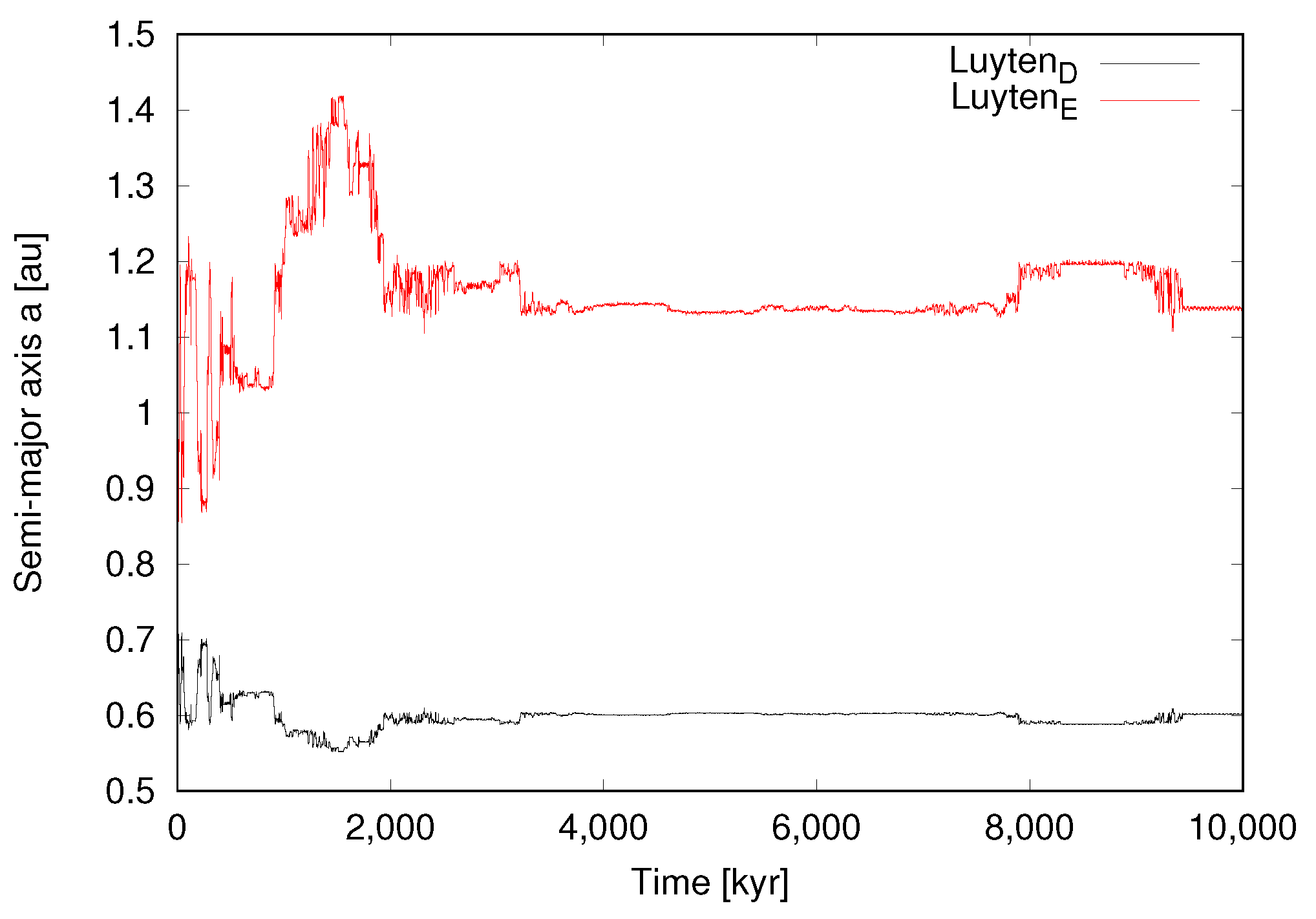
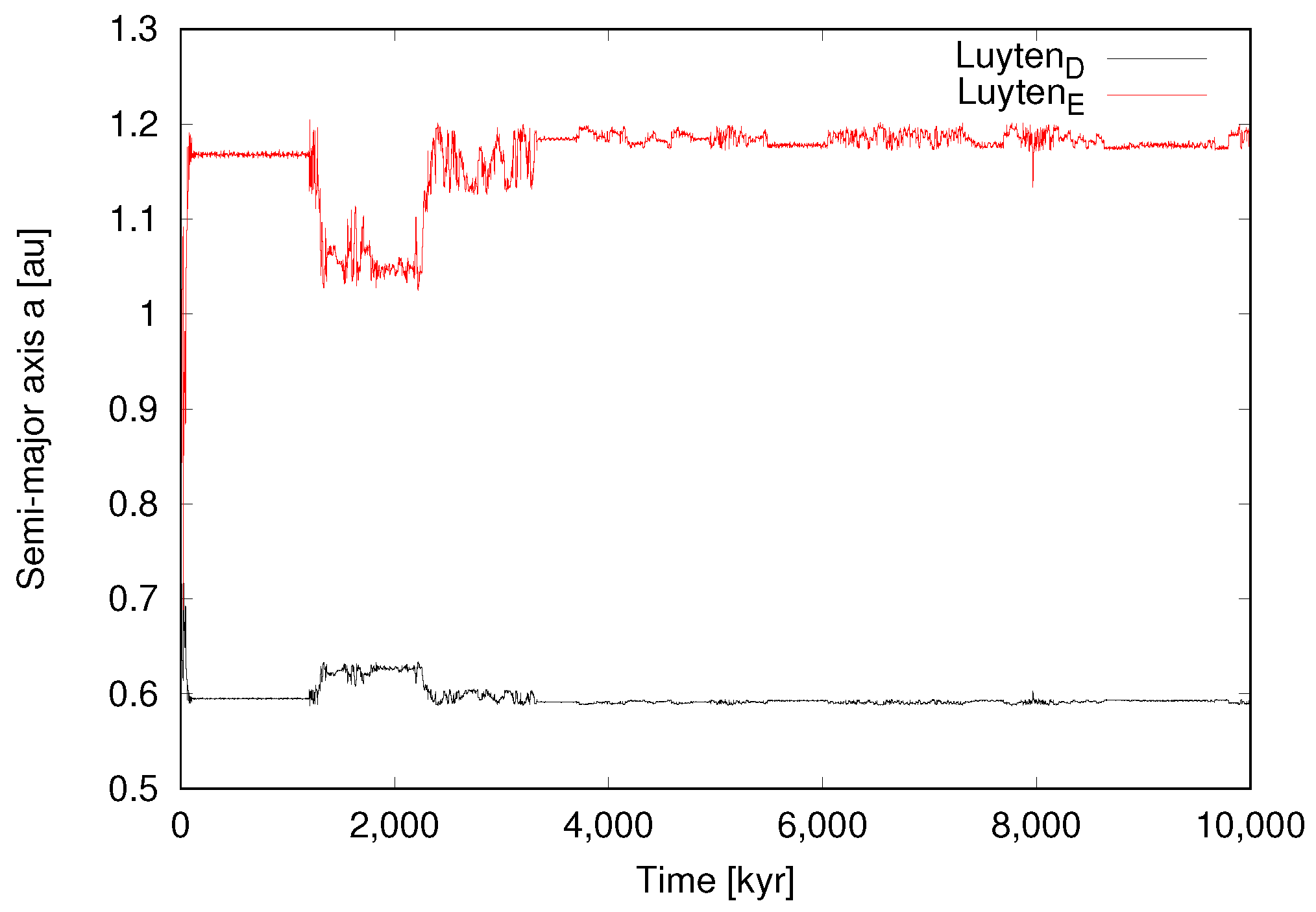
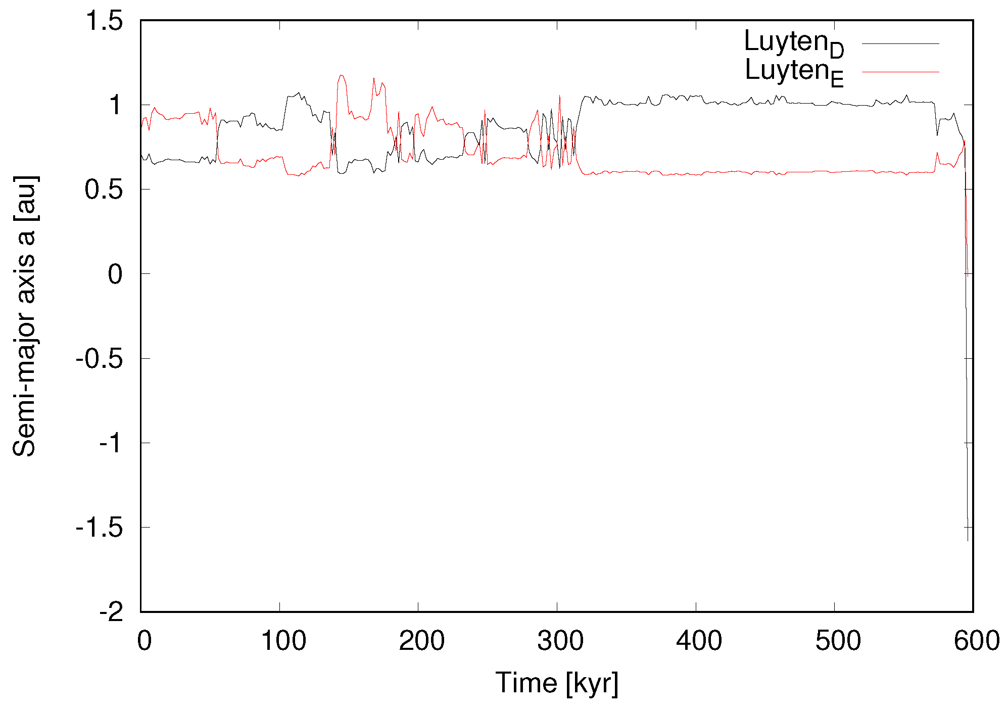
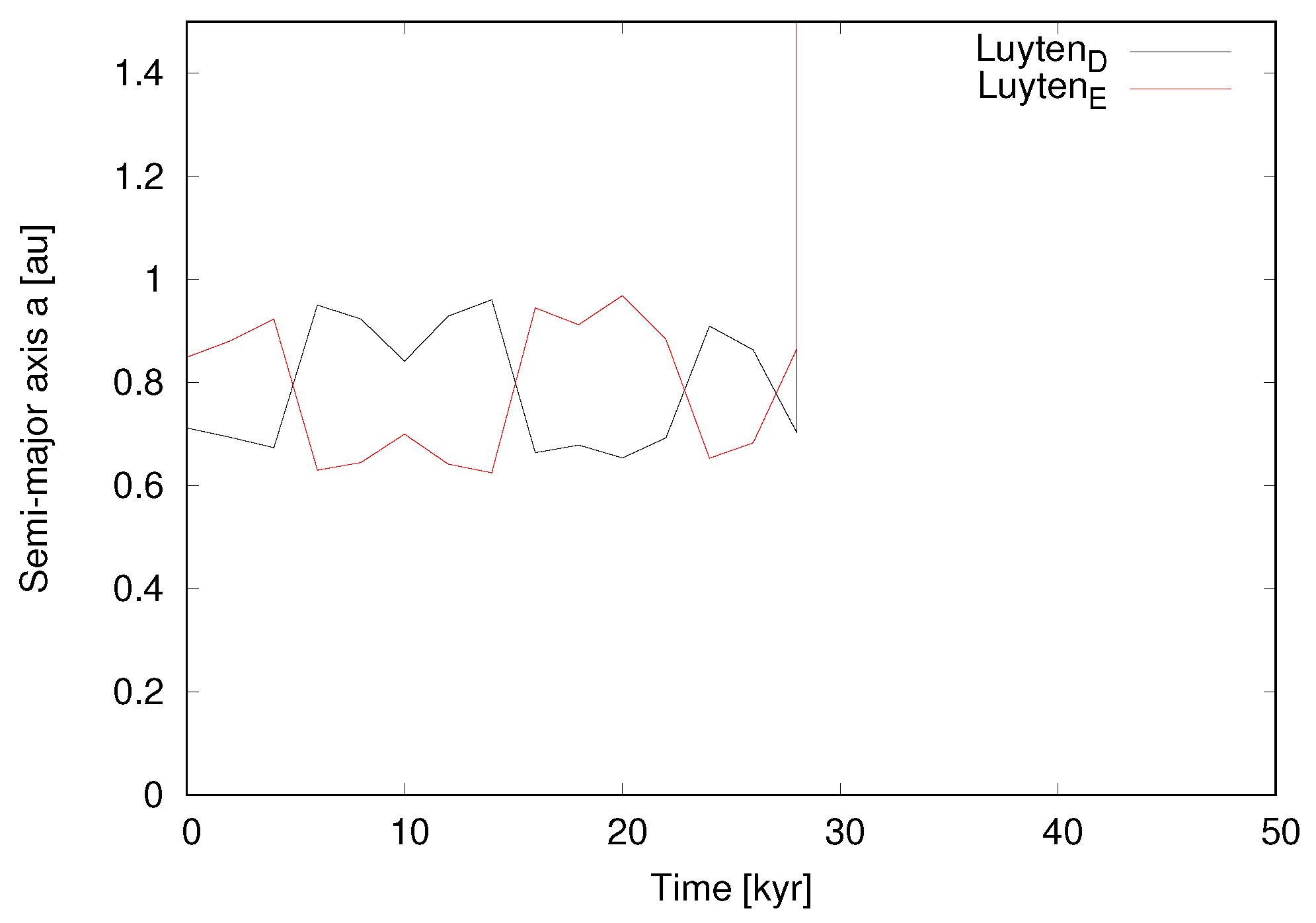
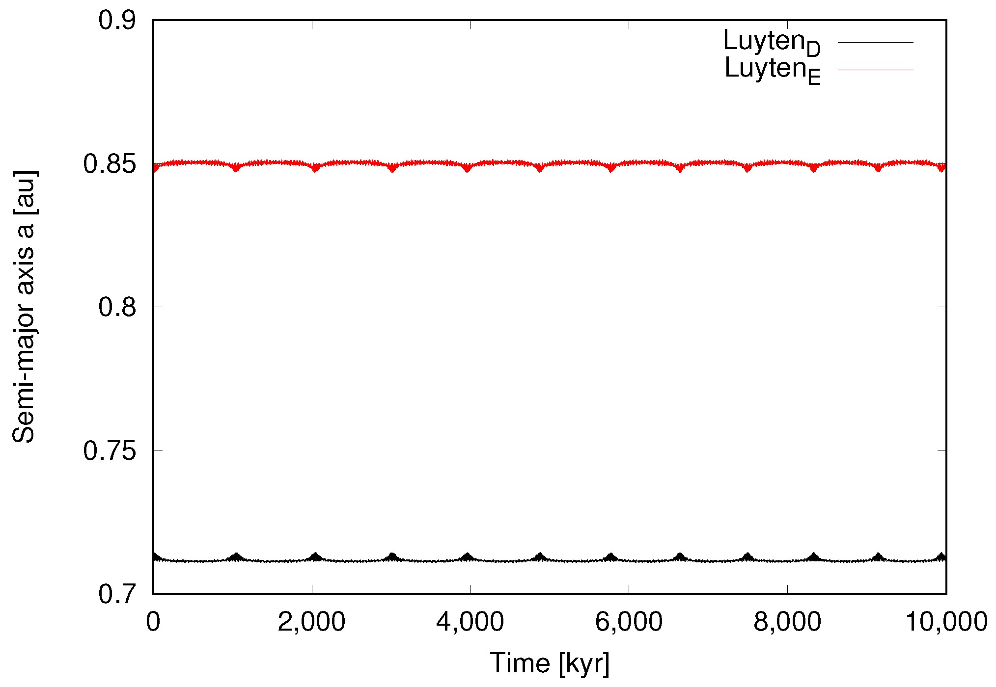
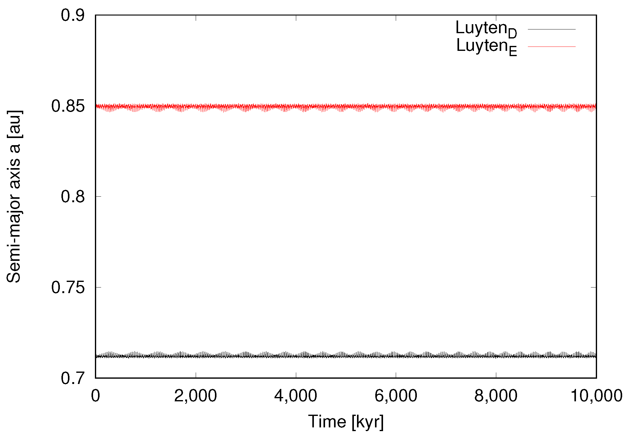
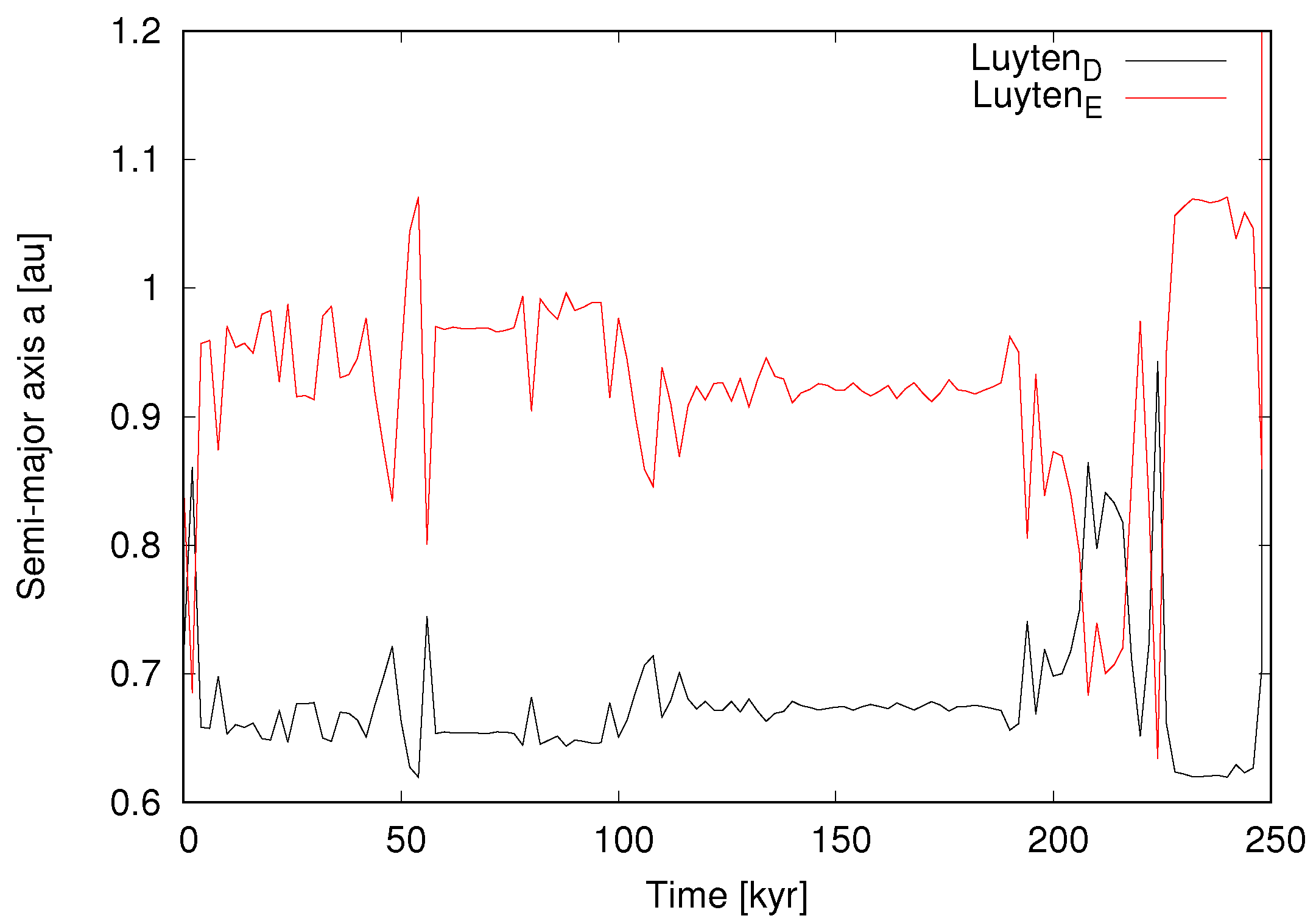
3.1. The Stability of the Planetary System

We show our results for the six cases (0–5) in Figure 1, Figure 2, Figure 3, Figure 4, Figure 5 and Figure 6, respectively. Assuming the nominal osculating elements shown in Table 1 (and including the range of values within error bars), our numerical integrations indicate that the two inner planets are and will remain stable. However, the opposite is true for the outer planets. Therefore, we consider that the most stable configuration for the outer planets is that with the highest possible eccentricity as the initial condition. This indeed corresponds to Case 5 (Figure 6), which is has the maximum eccentricity among the cases with stable orbits. Another stable configuration is Case 4 (Figure 5); however, it is not realistic to expect that any system would have perfectly circular orbits. Cases 0–3 represent unstable configurations. We note that Case 2 (Figure 3) resulted in an impact, and in Case 3 (Figure 4) both outer planets escape after a close encounter. The orbital integration of the nominal case clearly shows the instability of the system (Figure 7), which results in a collision.

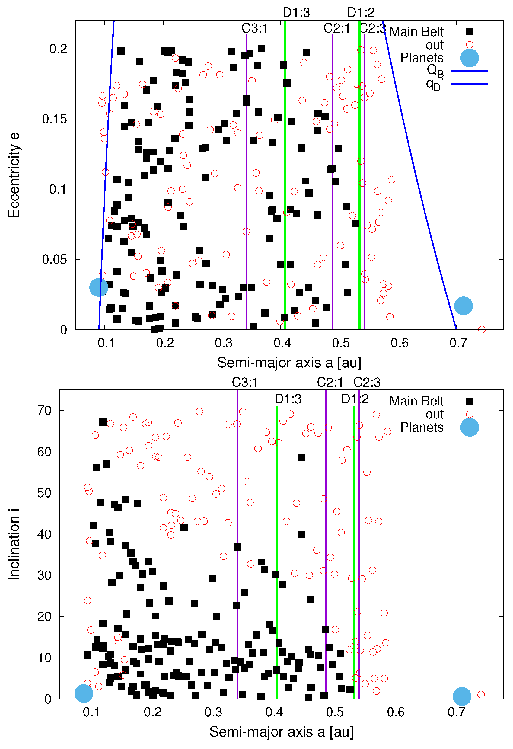
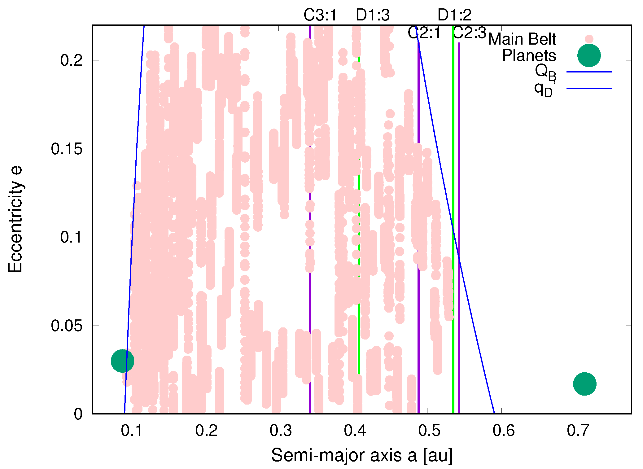
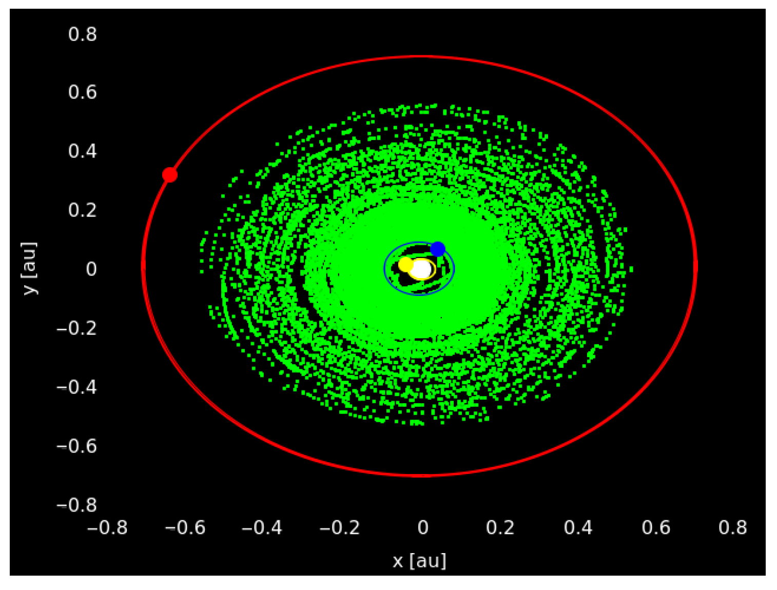
3.2. The Luyten Main Asteroid Belt

In Case 5, the main asteroid belt is an integral component of the Luyten’s system.

Table 3. Osculating elements of the four Luyten planets. Note that all angles are in units of degrees. M is mean anomaly.

Planet	a [au]	e	i	$\mathit{\omega }$	$\mathsf{\Omega }$	M
Luyten C	0.036	0.12	0.5	134.12	32.3	322
Luyten B	0.09	0.03	1.3	314.414	22.4	12.66
Luyten D	0.712	0.017	0.6	141.1515	151.5155	222.151
Luyten E	0.849	0.003	0.9	318.99515	43.5115	333.335

lists the osculating elements for the four Luyten planets. These produce the best case through integration.

We considered 200 sub-regions (each sub-region contains one synthetic asteroid) for the entire population with a semi-major axis between the following two limits 1: $Q_B<a_i<q_D$, and divided into 50 equal intervals (one interval is 0.0049826 au). Each sub-region was partitioned into four different segments having the following ranges of inclination: 0–$8.5^{\circ }$, 8.5–${17}^{\circ }$, 17–$43.5^{\circ }$ and 43.5–${70}^{\circ }$, similar to the main belt distribution in our solar system. We note that in terms of inclination, the asteroids of the solar system are situated between the ecliptic and ∼${70}^{\circ }$, with the majority of them residing below 17 degrees. The eccentricity is $e<0.2$, distributed randomly. This statistical difference has no relevance for the final results, and therefore will not create any notable bias.

The stable region is situated between the sweeping-zones of the planets. In particular, the outer portion is bounded by the mean-motion resonances D1:2 (at ∼$0.5348$ au) and C2:3 (at ∼$0.5434$ au), which are relatively close. In terms of semi-major axis, the bounds of the main belt are ∼$0.096$ au and ∼$0.535$ au, with an average semi-major axis of 0.229 au (

Table 4. The boundaries of the asteroid belts: maximum, minimum and average of the semi-proper elements. The values for the semi-major axis of the outer asteroid belt are biased by the input limits (maximum semi-major axis of the initial sample is $a=1.0$ au). The asterisk indicates that the maximum bound of the outer belt is determined from the initial conditions, but not computed.

Region	${\mathit{a}}_{\mathit{s}\mathit{p},\mathit{m}\mathit{i}\mathit{n}}$$<\mathit{a}>$${\mathit{a}}_{\mathit{s}\mathit{p},\mathit{m}\mathit{a}\mathit{x}}$ [au]	${\mathit{e}}_{\mathit{s}\mathit{p},\mathit{m}\mathit{i}\mathit{n}}$$<\mathit{e}>$${\mathit{e}}_{\mathit{s}\mathit{p},\mathit{m}\mathit{a}\mathit{x}}$	${\mathit{i}}_{\mathit{s}\mathit{p},\mathit{m}\mathit{i}\mathit{n}}$$<\mathit{i}>$${\mathit{i}}_{\mathit{s}\mathit{p},\mathit{m}\mathit{a}\mathit{x}}$
Main Belt	0.0959 0.2292 0.5294	0.0001 0.0984 0.2495	0.02 16.86 67.20
Outer Belt *	0.8515 33,000.4258 66,000.0000	<1

). For the osculating elements (average, maximum and minimum) in all stable asteroids, each output from full integration is for every 1 kyr.

Figure 8 shows the asteroids that remain on stable orbits (using the aforementioned initial configuration) until the end of the orbital integration considered for the belt. However, some of these asteroids will continue to remain stable (squares) or eventually become non-stable (circle-dots). The semi-major axes of three stable and surviving Luyten asteroids, MB1 (0.14014 au), MB2 (0.46318 au) and MB3 (0.15842 au) remain constant with time.

The majority of the asteroids lie in the region approaching the bound of the C3:1 mean-motion resonance (at ∼$0.3423$ au), the central core (the average region), and the more dense zone (the region with the highest density of asteroids) within 0.2292 au. We dub the latter the “hot-asteroids” because they are situated in the region of the belt that is closest to the star. The high inclination asteroids of the Luyten’s system are located in the region before the C2:1 mean motion resonance bound, at about 0.4485 au, with the majority of them being close to Luyten B (in semi-major axis). The latter are also part of the “hot-asteroid” population. The eccentricity distribution, even if it did contain a bias due to the choice of the maximum level, is rather homogeneous.

If we plot the orbital evolution of the stable asteroids in the synthetic main belt, we note the presence of a ‘hole’ (or a gap) in the central zone between about 0.26 au and 0.34 au in semi-major axis, eccentricity, $0.05<e<0.12$ and inclination $i>{23}^{\circ }$, where the C3:1 mean motion resonance lies. This is likely due to the combination of a secular resonance and the C3:1 mean motion resonance (Figure 9).

Verifying whether an asteroid belt could be present in this system can be initiated with a search for very large asteroids, or minor planets, because after collisions, such bodies generate asteroid families, or collisional asteroid families [11]. In light of that, we also investigated whether some very large asteroids could be observed with telescopes on Earth. Therefore, we assume that there is a Ceres-like body with radius $R_{ast}$∼1000 km. The probability that such body could be observed a priori when in transit with the Luyten’s star [12] is

$$p=\frac{R_{*}\pm R_a}{a}\frac{1}{1-e^2}$$

(1)

with the approximation of an edge-on observation ($i={90}^{\circ }$) and somewhere in the middle of the main asteroid belt, $a=\overline{a}=0.2292$ au and $e=0.0984$ (Table 4).

Knowing that $R_{*}=0.293R_{Sun}$ [1], the computed probability is approximately 1.3%, which is marginally smaller than the probability of finding (and observing) Luyten B (∼3%). However, this detection would have a very weak signal for a transit event. In fact, this corresponds to the radial-velocity semi-amplitude of $K=0.1$ cm/s, assuming the density of 2162.5 kg/m${}^3$ [13], which for a spherical body, gives the mass of ∼$9\times {10}^{21}$ kg. At present, it would not be possible to detect such a body (e.g., with ESPRESSO (the Echelle SPectrograph for Rocky Exoplanets and Stable Spectroscopic Observations), the detection threshold is 10 cm/s [14]). Even if we assume a rocky body, with the density similar to that of the Earth ($\rho =$ 5514 kg/m${}^3$), this leads to the semi-amplitude of $K<1$ cm/s. We computed the minimum limit of a large body to be at least 3500 km. This further validates the assertion that it would not be possible to detect a minor body in the Luyten’s main asteroid belt using present day observational techniques. The radial-velocity semi-amplitude computed via Equation (1) of [15], considering an inclination of $i={90}^{\circ }$.

3.3. Luyten’s Outer Asteroid Belt

The outer belt can host asteroids with more eccentric orbits and higher inclinations (Table 4). One might expect the size of an extra-solar Oort Cloud to be related to the Hill Sphere of the central star. In that case, the size of the extra-solar Oort Cloud would increase with stellar mass as $r_{max}\propto M^{1/3}$. However, the age of the star, its planetary architecture, and a possible membership in a star cluster can have a significant impact on the extent and mass of extra-solar Oort Clouds [16]. For our solar system, with 1 $M_{Sun}$ star, at distances of ${10}^5$ au or more, bodies become detached from the central star and may be lost to interstellar space. Therefore, we can expect that the Luyten’s system has a maximum extension of $r_{max,Luythen}={\displaystyle \frac{r_{max,Sun}{M}_{Luythen}^{1/3}}{M_{Sun}^{1/3}}}={10}^5\times 0.{29}^{1/3}\mathrm{au}\sim 6.6\times {10}^4\mathrm{au}$. Of course, this is a rough approximation, which does not take into account any external perturbations, such as the galactic tide or stellar close encounters, but it provides a general idea that the Luyten’s system can extend approximately 66,000 au.

We also found that some hyperbolic asteroids originated from both asteroid belts after close encounters with the planets and the star. This result emphasizes the possibility of the existence of hyperbolic bodies, which could travel to other systems and interact with them, i.e., ’Oumuamua [6] and 2i/Borisov [7].

3.4. Yarkovsky Effect in the Luyten’s System

Considering that the central star radiation (non-gravitational forces) is also present in extra-solar systems, we can calculate its effect on the Luyten planetary system.

Since the Yarkovsky effect depends on the radiation pressure (Equations (4) and (5) in Bottke, Vokrouhlický, Rubincam & Nesvorný [17]):

$$\frac{da}{dt}\propto \varphi ,$$

(2)

where $\varphi$ is the radiation pressure (radiation pressure coefficient):

$$\varphi =4\pi R^2{\xi }_0/\left(mc\right)$$

(3)

and ${\xi }_0$ is the solar radiation pressure:

$${\xi }_0\propto T^4.$$

(4)

Here, R is the radius, m is the mass, c is the speed of light, and T is the temperature of the star.

Therefore:

$$\varphi \propto T^4.$$

(5)

Finally,

$$\frac{da}{dt}\propto T^4.$$

(6)

We can approximately scale the Yarkovsky drift in the Luyten’s system—and in general in any extra-solar system—to the known Yarkovsky drift in our Solar System through scaling by the relative temperatures:

$$\frac{d{a}_{LS}}{dt}={\left[\frac{T_L}{T_S}\right]}^{4}d{a}_{SS}dt,$$

(7)

where $T_L=3382$ K and $T_S=5800$ K (efficiency temperature of the Sun). It follows that the Yarkovsky drift in the Luyten’ system can be found using that computed for our Solar System, so it can be approximated by the following relation:

$$\frac{d{a}_{LS}}{dt}\sim 0.117\frac{d{a}_{SS}}{dt}.$$

(8)

From [18] (Equation (2)) we know that

$$\frac{da}{dt}\propto \sqrt{a}(1-e^2)D,$$

(9)

where a, e and D are, respectively, the semi-major axis (in au), the eccentricity, and the diameter (in km) of the considered asteroid. Therefore, if $a_L$ and $e_L$, are the semi-major axis and the eccentricity, respectively, of the Luyten asteroid, then the Yarkovsky drift will be:

$$\frac{d{a}_{LS}}{dt}\sim 0.117\frac{\sqrt{a}(1-e^2)D}{\sqrt{a_L}(1-e_L^2)D_L}\frac{d{a}_{SS}}{dt}.$$

(10)

From this equation, we can approximate the Yarkovsky drift using the values for known asteroids with a specific range of osculating elements and with the range of orbits found in

Table 5. $D_R$ is the real diameter equal to the diameter of a real asteroid in the solar system, and $D_S$ is the diameter of a small asteroid (100 m). The acronyms used in this table are: YD—Yarkovsky drift, LS—Luyten’s system, MB—main asteroid belt, TLO—Trans-Luyten-Objects, SS—solar system. The YD, $da/dt$, is in ${10}^{-4}$ au/Myr. For the detailed description of the table entries, see the main text. Column 1: the YD of the MB asteroids and the Luyten MB asteroids. Column 2: the diameter, period, and density of the asteroid in the MB and a Luyten asteroid with the diameter of 100 m. Column 3: the semi-major axis of the asteroid in the MB, the YD of the Luyten belt asteroid of 100 m in the Luyten belt. Column 4: the eccentricity of the MB asteroid and the YD of the Luyten asteroid in the outer region, and the YD of the 100-m Luyten asteroid. Column 5: the YD drift of the Luyten TNO.

Solar Asteroid	$|{\mathit{d}\mathit{a}}_{\mathit{S}\mathit{S}}/\mathit{d}\mathit{t}|$	D [km]–P [h]–$\mathit{\rho }$ [g/cm${}^3$]	a [au]	e
Luyten Asteroid	$|{\mathit{d}\mathit{a}}_{\mathit{L}\mathit{S}}/\mathit{d}\mathit{t}|$	${\mathit{d}\mathit{a}}_{\mathit{S}\mathit{S},\mathit{r}\mathit{e}\mathit{s}\mathit{p},\mathit{M}\mathit{B}}/\mathit{d}\mathit{t}$	${\mathit{d}\mathit{a}}_{\mathit{S}\mathit{S},\mathit{m}\mathit{a}\mathit{x},\mathit{M}\mathit{B}}/\mathit{d}\mathit{t}$	${\mathit{d}\mathit{a}}_{\mathit{S}\mathit{S},\mathit{r}\mathit{e}\mathit{s}\mathit{p},\mathit{T}\mathit{L}\mathit{O}}/\mathit{d}\mathit{t}$	$\mathit{d}{\mathit{a}}_{\mathit{S}\mathit{S},\mathit{m}\mathit{a}\mathit{x},\mathit{T}\mathit{L}\mathit{O}}/\mathit{d}\mathit{t}$
	(${\mathit{D}}_{\mathit{R}}$)	(${\mathit{D}}_{\mathit{S}}$, ${\overline{\mathit{a}}}_{\mathit{M}\mathit{B}}$, ${\overline{\mathit{e}}}_{\mathit{M}\mathit{B}}$)	(${\mathit{a}}_{\mathit{m}\mathit{i}\mathit{n},\mathit{M}\mathit{B}}$)	(${\mathit{D}}_{\mathit{R}}$-${\mathit{D}}_{\mathit{S}}$, ${\overline{\mathit{a}}}_{\mathit{T}\mathit{L}\mathit{O}}$, ${\overline{\mathit{e}}}_{\mathit{T}\mathit{L}\mathit{O}}$)	(${\mathit{a}}_{\mathit{m}\mathit{i}\mathit{n},\mathit{T}\mathit{L}\mathit{O}}$)
(1685) Toro	1.38	3.5–10.2–2.5	1.367	0.436
“Toro Luyten”	0.32	11.29		0.21–7.38	15.50 (a = 0.132)
(161989) Cacus	1.60	1–3.8–2.5	1.123	0.214
“Cacus Luyten”	0.40	3.99		0.26–2.61	5.48
(2100) Ra-Shalom	2.21	2.3–?–1.7	0.832	0.437
“Ra-Shalom Luyten”	0.66	15.09		0.14–3.29	6.91
	Average		Max	Average	Max
Asteroid Luyten	0.51	10.12	23.3	0.20	15.5

. Additionally, we assume that the asteroids of the Luyten’s system are similar to those in our Solar System, and use the values from real measurements published by [19]. The maximum and minimum Yarkovsky drift in the Luyten’s system was found by considering the values of the semi-major axis and eccentricity of the possible belts. In Table 5, the first column shows the Yarkovsky drift of the main belt asteroids and the Yarkovsky drift of the Luyten main belt asteroids, respectively, in the first and second row. The second column includes the diameter, the period, and the density of the asteroid in the main belt (first row) and the Yarkovsky drift for a Luyten asteroid with the diameter of 100 m. The third column shows the semi-major axis of the asteroid in the main belt (first row), and the Yarkovsky drift of the Luyten belt asteroid of 100 m with the minimum semi-major axis and the maximum eccentricity possible in the Luyten belt (second row). The fourth column lists the eccentricity of the main belt asteroid (first row), and in the second row, the Yarkovsky drift of the Luyten asteroid in the outer region having the same diameter as that in the solar system and the Yarkovsky drift of the 100-m in size Luyten asteroid at an average semi-major axis and eccentricity. The last column shows the Yarkovsky drift of the Luyten TNO, with the minimum semi-major axis of the Luyten TNOs and minimum eccentricity possible.

The Yarkovsky drift and close encounters can lead to the asteroids to assume hyperbolic orbits. If such asteroids do not collide with the planets or the host star, they could escape from the system and enter another one, as it was recently documented in the case of now famous exo-asteroid ’Oumuamua [6].

If we consider that a drift 2 of 0.0003 au is enough to destabilize an asteroid, it follows that the Yarkovsky drift can induce chaoticity after about 0.588 Myr. This corresponds to 2.7 Myr in Earth cycles for kilometer-sized objects and less than 30 yrs (or 138 yrs in Earth cycles) for 100 meter-sized objects. Thus, the Luyten belt asteroid families can indeed exist. However, some of these families might persist only for short time, relative to our main belt, before losing their 100 m wide asteroids. Such asteroids are again possible candidates for hyperbolic orbits. Thus, for extrasolar systems like Luyten, it is easier to lose material towards other systems (and also towards their main star—Luyten A).

4. Conclusions

In this work, we investigated the possibility of the Luyten’s system (with the four planets), situated only 12.3 ly from our solar system, hosting one or more asteroid belts. Our results suggest that the Luyten planetary system is stable if the outer planets have an eccentricity configuration that is at least less than 0.1 or just far away enough so their orbits do not cross. In particular, we found stable orbits for 1/10 of the nominal eccentricity, $e=0.017$ for Luyten D and $e=0.003$ for Luyten E.

Our computations show that the inner planets remain in stable orbits for up to 10 Myr (equivalent to ∼316 Myr in Earth cycles), and the outer planets remain stable up to 100 Myr (corresponding to ∼74 Myr in Earth-cycles). The Luyten’s system could potentially host two asteroid belts confined within a well-defined range of orbital elements. The main, or inner, asteroid belt is situated between the planets Luyten B and Luyten D (a pictorial representation of the possible belt at the orbital plane can be seen in Figure 10).

The main asteroid belt is located between ∼0.0959 au and ∼$0.5294$ au from the central star. The central core of the belt is at 0.229 au (which is the average semi-major axis of the Luyten asteroids). The majority of the asteroids have their semi-major axis smaller than the C3:1 mean-motion resonance (at about 0.3423 au), the region which contains the central core, and the more dense zone just prior to 0.2292 au; we call these objects the “hot-asteroids” because they are the closest to the star in the belt. The Luyten’s system asteroids with high inclinations are located in the region that has its semi-major axis marginally smaller than the C2:1 mean motion resonance, at approximately 0.4485 au, with the majority situated next (in semi-major axis) to Luyten B, making them part of the “hot-asteroid” population. The eccentricity distribution is homogeneous. The apparent empty region caused by a secular resonance is situated between ∼0.26 au and ∼0.34 au in semi-major axis, eccentricity, $0.05<e<0.12$ and inclination $i>{23}^{\circ }$. The existence of the main asteroid belt might have arisen due to planetesimal leftovers after the formation of the system, and/or as a result of impacts on planets (or perhaps some other mechanisms). The outer asteroid belt, where the Trans-Luyten Objects lie, is confined between ∼0.852 au and ∼$6.6$ × ${10}^5$ au from the star. Some asteroids can escape, forming possible ’Omuamua-like objects.

The average Yarkovsky drift computed for the Luyten main belt is ${\displaystyle \frac{da}{dt}}=0.51\times {\displaystyle \frac{{10}^{-4}\mathrm{au}}{\mathrm{Myr}}}$, but for a 100 m-sized object, it is ${\displaystyle \frac{da}{dt}}=10.12\times {\displaystyle \frac{{10}^{-4} \mathrm{au}}{\mathrm{Myr}}}$. The action of the non-gravitational forces could quickly destroy the Luyten asteroid belt and eject the material out of their asteroid families in less than a half million years for the km-size objects, and less than a year for objects with a diameter equal to or less than 100 m. This demonstrates that for small asteroids in systems such as the Luyten, minor bodies can be ejected easily and quickly towards other systems, providing the source of ’Oumuamua or 2I/Borisov-like objects. Nevertheless, similar cases of exo-asteroids or exo-comets entering our Solar System and vice versa could take place.

Minor bodies in the Luyten asteroid belt are unlikely to be detected, but that does not preclude the possibility of their existence. We found that even a rocky Ceres-like body would not be detectable with the radial velocity method (we computed the minimum limit of a large body to be at least 3500 km).

The presence of asteroids is of immense importance because they can influence the evolution of the planets via impacts. For example, asteroidal impacts can affect planetary surfaces and atmospheres, and also deliver water and material necessary for the formation of life or conversely, have a destructive effect.

[custom] References

References

1. Astudillo-Defru, N.; Forveille, T.; Bonfils, X.; Sǵransan, D.; Bouchy, F.; Delfosse, X.; Lovis, C.; Mayor, M.; Murgas, F.; Pepe, F.; et al. The HARPS search for southern extra-solar planets-XLI. A dozen planets around the M dwarfs GJ 3138, GJ 3323, GJ 273, GJ 628, and GJ 3293. Astron. Astrophys. 2017, 602, A88. [Google Scholar] [CrossRef] [Green Version]
2. Pozuelos, F.J.; Suárez, J.C.; de Elía, G.C.; Berdiñas, Z.M.; Bonfanti, A.; Dugaro, A.; Gillon, M.; Jehin, E.; Günther, M.N.; Van Grootel, V.; et al. GJ 273: On the formation, dynamical evolution, and habitability of a planetary system hosted by an M dwarf at 3.75 parsec. Astron. Astrophys. 2020, 641, A23. [Google Scholar] [CrossRef]
3. Research Consortium On Nearby Stars (RECONS). The One Hundred Nearest Stars (Report). 2012. Available online: http://www.astro.gsu.edu/RECONS/TOP100.posted.htm (accessed on 25 November 2021).
4. Tuomi, M.; Jones, H.R.A.; Butler, R.P.; Arriagada, P.; Vogt, S.S.; Burt, J.; Laughlin, G.; Holden, B.; Shectman, S.A.; Crane, J.D.; et al. Frequency of planets orbiting M dwarfs in the Solar neighbourhood. arXiv 2019, arXiv:1906.04644. [Google Scholar]
5. Canup, R.M.; Asphaug, E. Origin of the Moon in a giant impact near the end of the Earth’s formation. Nature 2001, 412, 708–712. [Google Scholar] [CrossRef] [PubMed]
6. De la Fuente Marcos, C.; de la Fuente Marcos, R.; Aarseth, S.J. Where the Solar system meets the solar neighbourhood: Patterns in the distribution of radiants of observed hyperbolic minor bodies. Mon. Not. R. Astron. Soc. Lett. 2018, 476, L1–L5. [Google Scholar] [CrossRef] [Green Version]
7. Guzik, P.; Drahus, M.; Rusek, K.; Waniak, W.; Cannizzaro, G.; Pastor-Marazuela, I. Initial characterization of interstellar comet 2I/Borisov. Nat. Astron. 2020, 4, 53–57. [Google Scholar] [CrossRef] [Green Version]
8. Hanslmeier, A.; Dvorak, R. Numerical integration with Lie series. Astron. Astrophys. 1984, 132, 203. [Google Scholar]
9. Eggl, S.; Dvorak, R. Lecture Notes in Physics; Springer: Berlin, Germany, 2020; Volume 790, p. 431. [Google Scholar]
10. Galiazzo, M.A.; Bazsò, Á; Dvorak, R. Fugitives from the Hungaria region: Close encounters and impacts with terrestrial planets. Planet. Space Sci. 2013, 84, 5–13. [Google Scholar] [CrossRef] [Green Version]
11. Carruba, V.; Nesvorný, D.; Aljbaae, S.; Domingos, R.C.; Huaman, M. On the oldest asteroid families in the main belt. Mon. Not. R. Astron. Soc. 2016, 458, 3731–3738. [Google Scholar] [CrossRef] [Green Version]
12. Perriman, M. The Exoplanet Handbook, 2nd ed.; Cambridge University Press: Cambridge, UK, 2018; p. 952. [Google Scholar]
13. Park, R.; Konopliv, A.; Bills, B.; Castillo-Rogez, J.; Asmar, S.; Rambaux, N.; Raymond, C.; Russell, C.; Zuber, M.; Ermakov, A.; et al. Gravity Science Investigation of Ceres from Dawn EGU, 2016, 18.8395P. Available online: https://meetingorganizer.copernicus.org/EGU2016/EGU2016-8395-1.pdf (accessed on 25 November 2021).
14. Mégevand, D.; Herreros, J.M.; Zerbi, F.; Cabral, A.; Di Marcantonio, P.; Lovis, C.; Pepe, F.; Cristiani, S.; Rebolo, R.; Santos, N.C. ESPRESSO: Projecting a rocky exoplanet hunter for the VLT. In Proceedings of SPIE—The International Society for Optical Engineering; SPIE: San Diego, CA, USA, 2010; p. 7735. [Google Scholar]
15. Cumming, A.; Marcy, G.W.; Butler, R.P. The Lick planet search: Detectability and mass thresholds. Astrophys. J. 1999, 526, 890. [Google Scholar] [CrossRef] [Green Version]
16. Baxter, E.J.; Blake, C.H.; Jain, B. Probing Oort clouds around Milky Way stars with CMB surveys. Astron. J. 2018, 156, 243. [Google Scholar] [CrossRef] [Green Version]
17. Bottke, W.F., Jr.; Vokrouhlický, D.; Rubincam, D.P.; Nesvorný, D. The Yarkovsky and YORP effects: Implications for asteroid dynamics. Annu. Rev. Earth Planet. Sci. 2006, 34, 157–191. [Google Scholar] [CrossRef] [Green Version]
18. Del Vigna, A.; Faggioli, L.; Milani, A.; Spoto, F.; Farnocchia, D.; Carry, B. Detecting the Yarkovsky effect among near-Earth asteroids from astrometric data. Astron. Astrophys. 2018, 617, A61. [Google Scholar] [CrossRef] [Green Version]
19. Farnocchia, D.; Chesley, S.R.; Vokrouhlický, D.; Milani, A.; Spoto, F.; Bottke, W.F. Near Earth asteroids with measurable Yarkovsky effect. Icarus 2013, 224, 1–13. [Google Scholar] [CrossRef] [Green Version]
20. Knezević, Z.; Milani, A. (Eds.) Dynamics of Populations of Planetary Systems (IAUC 197). In Proceedings of the International Astronomical Union; Cambridge University Press: Cambridge, UK, 2015; ISBN 0-521-85203-X. [Google Scholar]
21. Galiazzo, M.A.; Wiegert, P.; Aljbaae, S. Influence of the Centaurs and TNOs on the main belt and its families. Astrophys. Space Sci. 2016, 361, 371. [Google Scholar] [CrossRef] [Green Version]
Figure 1. Case 0 ( e D = 0.0085, e E = nominal). Time evolution of the two outer planets over 10 Myr. This is unstable configuration.
Universe 08 00190 g001
Figure 2. Case 1 ( e D = 0.085, e E = nominal). Time evolution of the two outer planets over 10 Myr. This is unstable configuration.
Universe 08 00190 g002
Figure 3. Case 2 ( e D = nominal, e E = 0.015). Time evolution of the two outer planets over 10 Myr. In this unstable configuration, the planets end up colliding.
Universe 08 00190 g003
Figure 4. Case 3 ( e D = 0.0085, e E = nominal). Time evolution of the two outer planets over 10 Myr. In this unstable configuration the planets escape after undergoing a close encounter.
Universe 08 00190 g004
Figure 5. Case 4 ( e D = 0, e E = 0). Time evolution of the two outer planets over 10 Myr. While this is a stable configuration, it is not realistic to expect that any system will have perfectly circular orbits.
Universe 08 00190 g005
Figure 6. Case 5 ( e D = 0.017, e E = 0.003). Time evolution of the two outer planets over 10 Myr. This is the most stable configuration.
Universe 08 00190 g006
Figure 7. Nominal case ( e D = 0.17, e E = 0.03): Time evolution of the two outer planets over 10 Myr. This configuration is also unstable, resulting in a collision.
Universe 08 00190 g007
Figure 8. Luyten main asteroid belt (semi-proper elements) in the plane a e plane (top) and a i plane (bottom). Some of the asteroids will remain stable (squares) or eventually become non-stable (circle-dots). The vertical lines are the two main mean motion resonances with the planets Luyten D and Luyten E.
Universe 08 00190 g008
Figure 9. Orbital evolution of the Luyten main asteroid belt (semi-proper elements) in the phase planes a e and a i . The vertical lines are the two main mean motion resonances with the planet Luyten D and Luyten E. Note the presence of a ’hole’ in the central zone between 0.26–0.34 au in semi-major axis, and eccentricity 0.05 < e < 0.12 . This is likely due to the combination of a secular resonance and the C3:1 mean motion resonance.
Universe 08 00190 g009
Figure 10. Luyten’s main asteroid belt in the plane at i = 0 .
Universe 08 00190 g010