
Bulk Viscous Flat FLRW Model with Observational Constraints in f(T, B) Gravity


Abstract
1. Introduction
2. Basic Formalism of Gravity
Bulk Viscosity
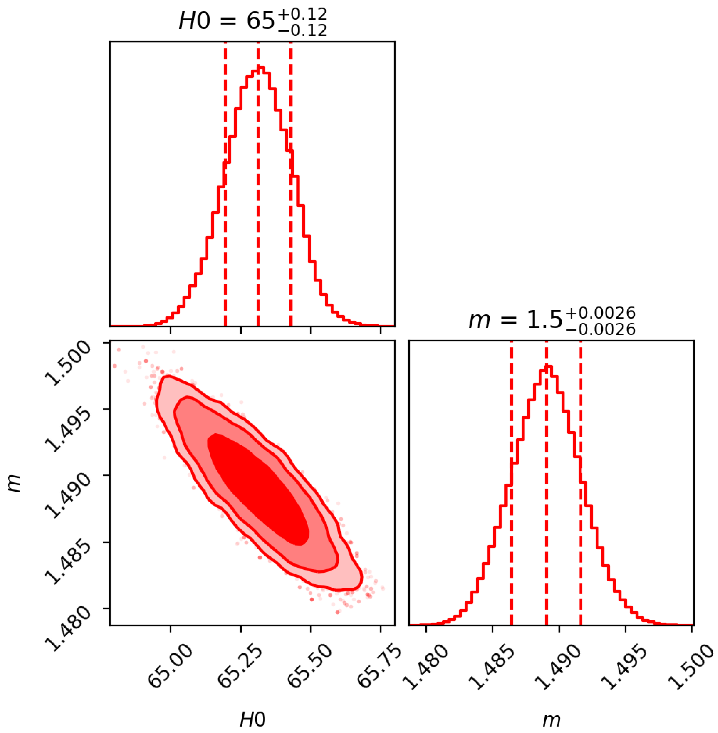
3. Cosmological Model with Observational Constraints
4. Dynamical Parameters and Their Physical Discussion for Viscous Fluid
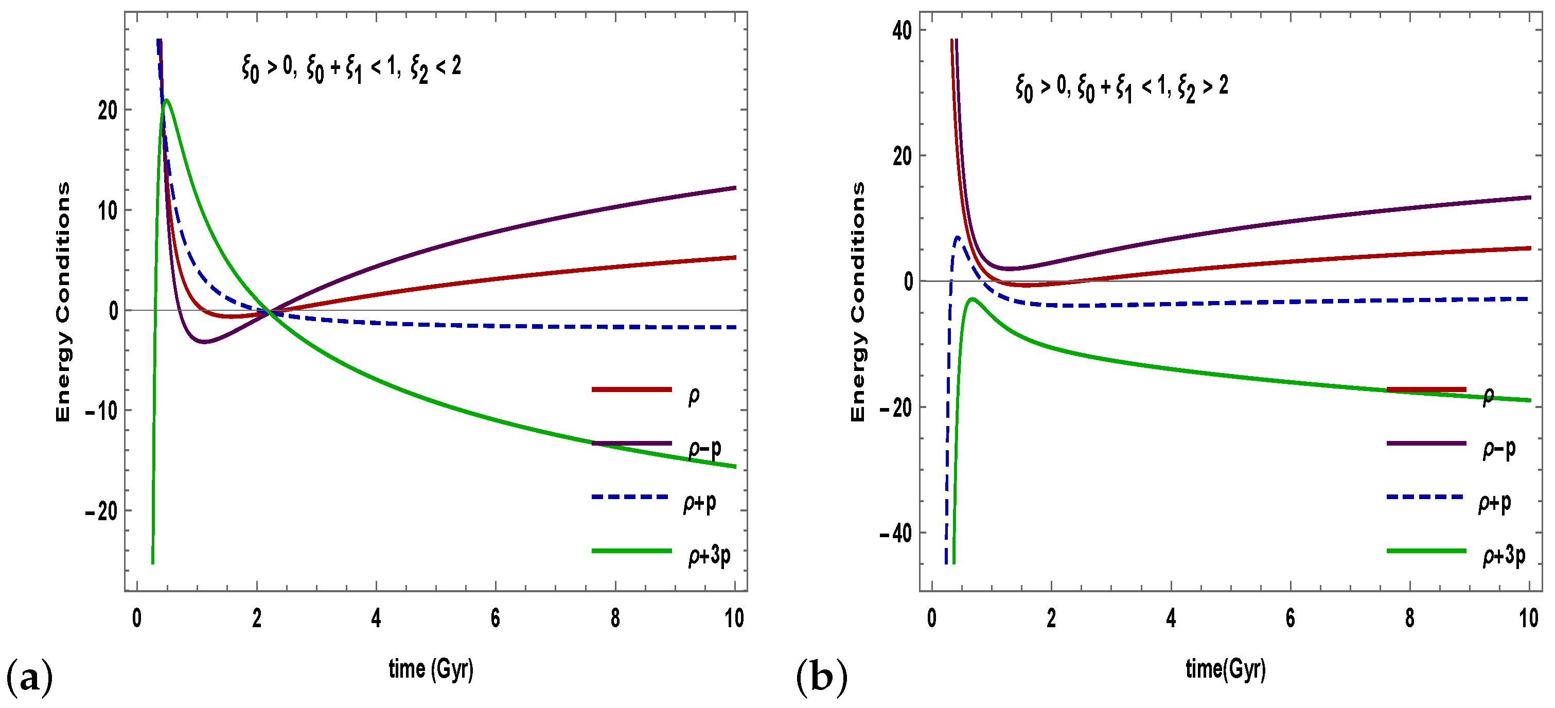
5. Energy Condition
- Null energy condition (NEC) if
- Weak energy conditions (WEC) if
- Strong energy conditions (SEC) if , ;
- Dominant energy conditions (DEC) if ,
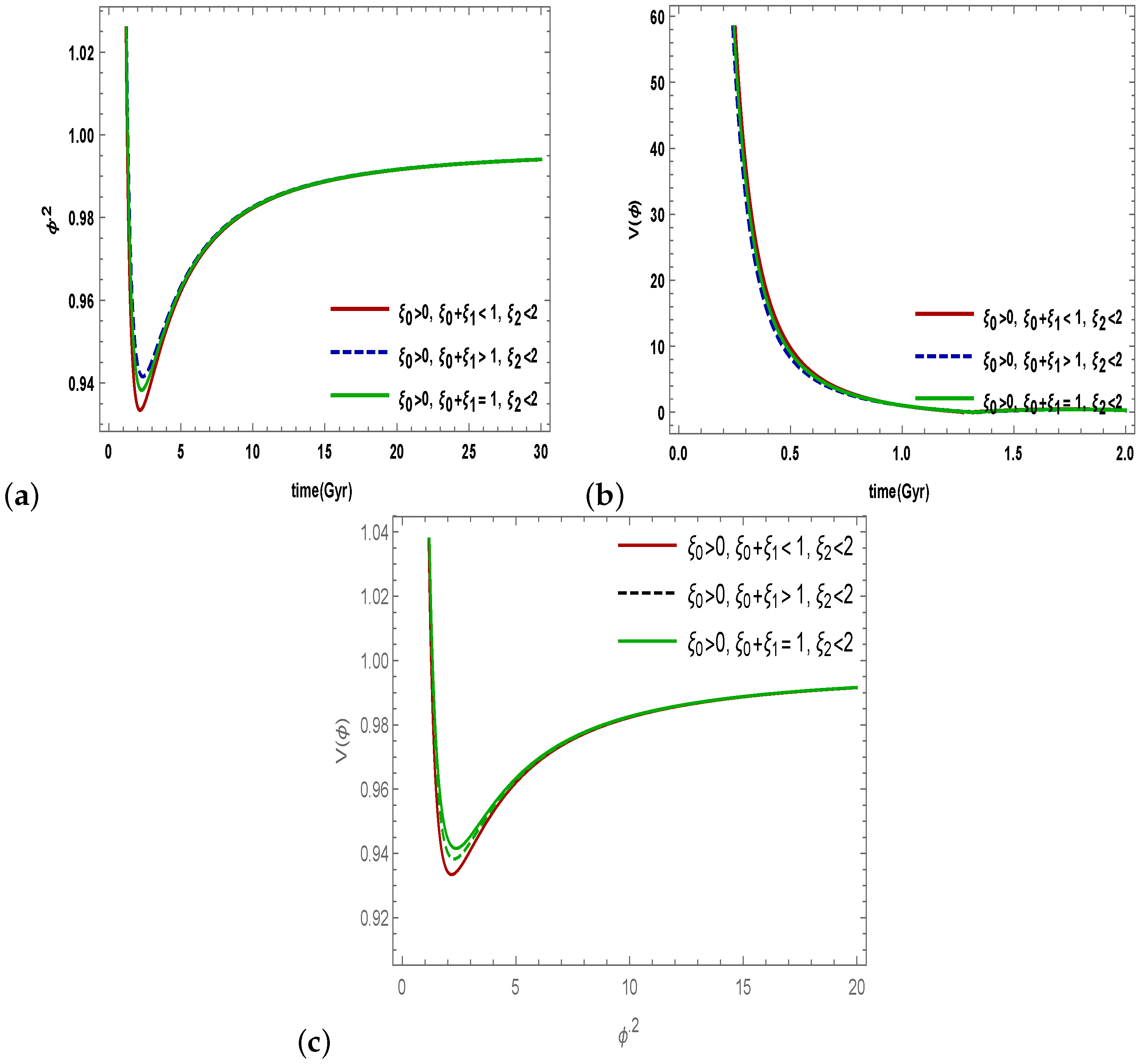
6. Tachyon Model
7. Conclusions
- Figure 3 shows the effective equation of state parameter involving the bulk viscous pressure . The evolutionary trajectory of the EoS parameter exhibits quintom-like behavior (transition from phantom to quintessence and evolution of the LCDM limit) for the limiting conditions of the viscosity parameter shown in (Figure 3a).
- We have seen that the viscous EoS parameter achieves a phantom-like universe for a particular choice of for shown in (Figure 3b). Thus, the viscous EoS parameter represents a DE-dominated universe for all the models depending upon model parameters. This behavior is compatible with the gravity model.
- Figure 4 shows the temporal evolution of the energy conditions. Keep in mind that to serve the late-time acceleration of the universe, the SEC has to violate. The SEC is the most discussed of all the energy conditions. According to recent findings from the speeding universe, the SEC must be violated on a cosmological scale. In our derived model, NEC, WEC, and DEC satisfy the criteria established from the Raychaudhuri equations. However, SEC is violated. As a consequence, our model is accurate and its solutions are physically feasible.
- Figure 5 depicts the correspondence between the scalar field and the gravity model. We have noticed that the scalar field increases and potential decreases as time increases. The corresponding potential function exhibits a positive but decreasing relationship with time. Later, the scalar field exhibits inverse proportionality to its decreasing behavior from its maximum. In the brane-world cosmology, this kind of behavior corresponds to scaling solutions.
Author Contributions
Funding
Data Availability Statement
Acknowledgments
Conflicts of Interest
References
- Perlmutter, S.; Aldering, G.; Goldhaber, G.; Knop, R.A.; Nugent, P.; Castro, P.G.; Deustua, S.; Fabbro, S.; Goobar, A.; Groom, D.E.; et al. Measurements of Ω and Λ from 42 high-redshift supernovae. Astrophys. J. 1999, 517, 565–586. [Google Scholar] [CrossRef]
- Riess, A.G.; Filippenko, A.V.; Challis, P.; Clocchiatti, A.; Diercks, A.; Garnavich, P.M.; Gilliland, R.L.; Hogan, C.J.; Jha, S.; Kirshner, R.P.; et al. Observational evidence from supernovae for an accelerating universe and a cosmological constant. Astron. J. 1998, 116, 1009–1038. [Google Scholar] [CrossRef]
- Ade, P.A.; Aghanim, N.; Ahmed, Z.; Aikin, R.W.; Alexander, K.D.; Arnaud, M.; Aumont, J.; Baccigalupi, C.; Banday, A.J.; Barkats, D.; et al. Joint analysis of BICEP2/Keck Array and Planck data. Phys. Rev. Lett. 2015, 114, 101301. [Google Scholar] [CrossRef] [PubMed]
- Ade, P.A.; Aghanim, N.; Arnaud, M.; Ashdown, M.; Aumont, J.; Baccigalupi, C.; Banday, A.J.; Barreiro, R.B.; Bartlett, J.G.; Bartolo, N.; et al. Planck 2015 results XIII. Cosmological parameters. Astron. Astrophys. 2016, 594, A13. [Google Scholar]
- Clifton, T.; Ferreira, P.G.; Padilla, A.; Skordis, C. Modified gravity and cosmology. Phys. Rep. 2012, 513, 1–189. [Google Scholar] [CrossRef]
- Nojiri, S.; Odintsov, S.D. Introduction to modified gravity and gravitational alternative for dark energy. Int. J. Geom. Methods Mod. 2007, 4, 115. [Google Scholar] [CrossRef]
- Starobinsky, A.A. A new type of isotropic cosmological models without singularity. Phys. Lett. B 1980, 91, 99. [Google Scholar] [CrossRef]
- Nojiri, S.; Odintsov, S.D. Unified cosmic history in modified gravity: From f(R) theory to Lorentz non-invariant models. Phys. Rep. 2011, 505, 59. [Google Scholar] [CrossRef]
- Glavan, D.; Lin, C. Einstein-Gauss-Bonnet gravity in four-dimensional spacetime. Phys. Rev. Lett. 2020, 124, 081301. [Google Scholar] [CrossRef]
- Harko, T.; Lobo, F.S.N.; Nojiri, S.; Odintsov, S.D. f(R,T) gravity. Phys. Rev. D 2011, 84, 024020. [Google Scholar] [CrossRef]
- Odintsov, S.D.; Oikonomou, V.K.; Fronimos, F.P. Rectifying Einstein-Gauss-Bonnet inflation in view of GW170817. Nucl. Phys. B 2020, 958, 115135. [Google Scholar] [CrossRef]
- Anagnostopoulos, F.K.; Basilakos, S.; Saridakis, E.N. Bayesian analysis of f(T) gravity using f σ 8 data. Phys. Rev. D 2019, 100, 083517. [Google Scholar] [CrossRef]
- Unzicker, A.; Case, T. Translation of Einstein’s attempt of a unified field theory with teleparallelism. arXiv 2005, arXiv:arXiv:physics/0503046. [Google Scholar]
- Hayashi, K.; Shirafuji, T. New general relativity. Phys. Rev. D 1979, 19, 3524. [Google Scholar] [CrossRef]
- Pradhan, A.; Dixit, A. Anisotropic MHRDE model in BD theory of gravitation. Int. J. Geom. Methods Mod. 2019, 16, 1950185. [Google Scholar] [CrossRef]
- Dixit, A.; Pradhan, A. Stability, dark energy parameterization and swampland aspect of Bianchi type-VIh cosmological models with f(R,T)-gravity. Int. J. Geom. Methods Mod. 2020, 17, 2050213. [Google Scholar] [CrossRef]
- Samanta, G.C.; Godani, N. Physical parameters for stable f(R) models. Indian J. Phys. 2021, 94, 1303. [Google Scholar] [CrossRef]
- Pradhan, A.; Maurya, D.C.; Dixit, A. Dark energy nature of viscus universe in f(R)-gravity with observational constraints. Int. J. Geom. Methods Mod. Phys. 2021, 18, 2150124. [Google Scholar] [CrossRef]
- Ferraro, R.; Fiorini, F. Modified teleparallel gravity: Inflation without an inflaton. Phys. Rev. D 2007, 75, 084031. [Google Scholar] [CrossRef]
- Bamba, K.; Geng, C.Q.; Lee, C.C.; Luo, L.W. Equation of state for dark energy in f(T) gravity. J. Cosmol. Astropart. Phys. 2011, 01, 021. [Google Scholar] [CrossRef]
- Golovnev, A.; Guzman, M.-J. Approaches to spherically symmetric solutions in f(T) gravity. Universe 2021, 7, 121. [Google Scholar] [CrossRef]
- Pfeifer, C.; Schuster, S. Static spherically symmetric blacl holes in week f(T)- gravity. Universe 2021, 7, 153. [Google Scholar] [CrossRef]
- Bahamonde, S.; Capozziello, S. Noether symmetry approach in f(T,B) teleparallel cosmology. Eur. Phys. J. C 2017, 77, 1–10. [Google Scholar] [CrossRef] [PubMed]
- Escamilla, C.R.; Said, J.L. Cosmological viable models in f(T,B) theory as solutions to the H0 tension. Class Quantum Gravi. 2020, 37, 165002. [Google Scholar] [CrossRef]
- Shekh, S.H.; Chirde, V.R.; Sahoo, P.K. Energy conditions of the f(T,B) gravity dark energy model with the validity of thermodynamics. Comm.Theor. Phys. 2020, 22, 085402. [Google Scholar] [CrossRef]
- Godani, N. Locally rotationally symmetric Bianchi type-II cosmological model in f(R,T) gravity. Ind. J. Phys. 2019, 93, 951. [Google Scholar] [CrossRef]
- Pradhan, A.; Garg, P.; Dixit, A. FRW cosmological models with cosmological constant in f(R,T) theory of gravity. Can. J. Phys. 2021, 99, 741. [Google Scholar] [CrossRef]
- Tiwari, R.K.; Beesham, A.; Mishra, S.; Dubey, V. Anisotropic cosmological model in a modified theory of gravitation. Universe 2021, 7, 226. [Google Scholar] [CrossRef]
- Bhardwaj, V.K.; Pradhan, A. Evaluation of cosmological models in f(R,T) gravity in different dark energy scenario. New Astron. 2022, 91, 101675. [Google Scholar] [CrossRef]
- Tangphati, T.; Hansraj, S.; Banerjee, A.; Pradhan, A. Quark stars in f(R,T) gravity with an interacting quark equation of state. Phys. Dark Univ. 2022, 35, 100990. [Google Scholar] [CrossRef]
- Pretel, J.M.Z.; Tangphati, T.; Banerjee, A.; Pradhan, A. Charged quark stars in f(R,T) gravity. Chin. Phys. C 2022, 46, 115103. [Google Scholar] [CrossRef]
- Pradhan, A.; Dixit, A. The model of the transit cosmology along with observational constraints in f(Q,T) gravity. Int. J. Geom. Methods Mod. 2021, 18, 2150159. [Google Scholar] [CrossRef]
- Godani, N.; Samanta, G.C. FRW cosmology in f(Q,T) gravity. Int. J. Geom. Methods Mod. 2021, 18, 2150134. [Google Scholar] [CrossRef]
- Nojiri, S.; Odintsov, S.D.; Tretyakov, P.V. From inflation to dark energy in the non-minimal modified gravity. Prog. Theor. Phys. Suppl. 2008, 172, 81. [Google Scholar] [CrossRef]
- Elizalde, E.; Myrzakulov, R.; Obukhov, V.V.; Saez-Gomez, D. ΛCDM epoch reconstruction from F(R,G) and modified Gauss-Bonnet gravities. Class. Quantum Gravity 2010, 27, 095007. [Google Scholar] [CrossRef]
- Banerjee, A.; Pradhan, A.; Tangphati, T.; Rahaman, F. Wormhole geometry in f(Q) gravity and the energy conditions. Eur. Phys. J. C 2021, 81, 10131. [Google Scholar] [CrossRef]
- Gupta, S.; Dixit, A.; Pradhan, A. Tsallis holographic dark energy scenario in viscous F(Q) gravity and techyan field. Int. J. Geom. Methods Mod. 2022. [Google Scholar] [CrossRef]
- Pradhan, A.; Dixit, A.; Maurya, D.C. Quintessence behaviour of an anisotropic bulk viscous cosmological model in modified f(Q) gravity. arXiv 2022, arXiv:2210.13730. [Google Scholar]
- Iosifidis, D.; Myrzakulov, N.; Myrzakulov, R. Metric-affine version of Myrzakulov F(R,T,Q,τ) gravity and cosmological applications. Universe 2021, 7, 262. [Google Scholar] [CrossRef]
- Mardan, S.A.; Amjad, A.; Noureen, I. Frameworks of generalized anisotropic conformally flat polytropes in f(R) gravity. Eur. Phys. J. C 2022, 82, 794. [Google Scholar] [CrossRef]
- Noureen, I.; Arshad, N.; Mardan, S.A. Development of local density perturbation scheme in f(R) gravity to identify cracking points. Eur. Phys. J. C 2022, 82, 621. [Google Scholar] [CrossRef]
- Noureen, I.; Haq, U.; Mardan, S.A. Impact of f(R,T) gravity in evolution of charged viscous fluids. Int. J. Mod. Phys. D 2021, 30, 2150027. [Google Scholar] [CrossRef]
- Franco, G.A.; E-Rivera, C.; Levi Said, J. Stability analysis for cosmological models in f(T,B) gravity. Eur. Phys. J. C 2020, 80, 1. [Google Scholar] [CrossRef]
- Paliathanasis, A. Anisotropic spacetimes in f(T,B) theory I: Bianchi I universe. Eur. Phys. J. C 2022, 137, 1. [Google Scholar] [CrossRef]
- Shekh, S.H.; Moraes, H.R.S.; Sahoo, P.K. Physical acceptability of the Renyi, Tsallis and Sharma-Mittal holographic dark energy models in the f(T,B) gravity under Hubble’s cutoff. Universe 2021, 7, 67. [Google Scholar] [CrossRef]
- Escamilla-Rivera, C.; Rave-franco, G.; Levi-Said, J. f(T,B) cosmography for high redshifts. Universe 2021, 7, 441. [Google Scholar] [CrossRef]
- Li, B.; Sotiriou, T.P.; Barrow, J.D. f(T) gravity and local Lorentz invariance. Phys. Rev. D 2011, 83, 064035. [Google Scholar] [CrossRef]
- Krssak, M.; Saridakis, E.N. The covariant formulation of f(T) gravity. Class. Quant. Grav. 2016, 33, 115009. [Google Scholar] [CrossRef]
- Paliathanasis, A. de Sitter and Scaling solutions in a higher-order modified teleparallel theory. JCAP 2017, 1708, 027. [Google Scholar] [CrossRef]
- Karpathopoulos, L.; Basilakos, S.; Leon, G.; Paliathanasis, A.; Tsamparlis, M. Cartan symmetries and global dynamical systems analysis in a higher-order modified teleparallel theory. Gen. Rel. Gravity 2018, 50, 79. [Google Scholar] [CrossRef]
- Caruana, M.; Farrugia, G.; Said, J.L. Cosmological bouncing solutions in f(T,B) gravity. Eur. Phys. J. C 2020, 80, 1. [Google Scholar] [CrossRef]
- Paliathanasis, A. Cosmological evolution and exact solutions in a fourth-order theory of gravity. Phys. Rev. D 2017, 95, 064062. [Google Scholar] [CrossRef]
- Paliathanasis, A.; Leon, G. Cosmological evolution in f(T,B) gravity. Eur. Phys. J. Plus 2021, 136, 1. [Google Scholar] [CrossRef]
- Rave-Franco, G.A.; Escamilla-Rivera, C.; Said, J.L. Dynamical complexity of the teleparallel gravity cosmology. Phys. Rev. D 2021, 103, 084017. [Google Scholar] [CrossRef]
- Paliathanasis, A.; Leon, G. f(T,B) gravity in a Friedmann-Lemaî tre-Robertson-Walker universe with nonzero spatial curvature. arXiv 2022, arXiv:2201.12189. [Google Scholar]
- Paliathanasis, A. Minisuperspace Quantization of f(T,B) Cosmology. Universe 2021, 7, 150. [Google Scholar] [CrossRef]
- Najera, S.; Aguilar, A.; Rave-Franco, G.A.; Escamilla-Rivera, C.; Sussman, R.A. Inhomogeneous solutions in f(T,B) gravity. Int. J. Geom. Methods Mod. 2022, 2240003. [Google Scholar] [CrossRef]
- Ren, J.; Meng, X.H. Cosmological model with viscosity media (dark fluid) described by an effective equation of state. Phys. Lett. B 2006, 633, 1. [Google Scholar] [CrossRef]
- Tawfik, A.; Harko, T. Quark-hadron phase transitions in the viscous early universe. Phys. Rev. D 2012, 85, 084032. [Google Scholar] [CrossRef]
- Sharif, M.; Rani, S. Viscous dark energy in f(T) gravity. Mod. Phys. Lett. A 2013, 28, 1350118. [Google Scholar] [CrossRef]
- Singh, C.P.; Kumar, P. Friedmann model with viscous cosmology in modified f(R,T) gravity theory. Eur. Phys. J. C 2014, 74, 3070. [Google Scholar] [CrossRef]
- Bahamonde, S.; Dialektopoulos, K.F.; Escamilla-Rivera, C.; Farrugia, G.; Gakis, V.; Hendry, M.; Hohmann, M.; Said, J.L.; Mifsud, J.; Di Valentino, E. Teleparallel gravity: From theory to cosmology. arXiv 2021, arXiv:2106.13793. [Google Scholar] [CrossRef] [PubMed]
- Bahamonte, S.; Boehmer, C.G.; Wight, M. Modified teleparallel theories of gravity. Phys. Rev. D 2015, 9, 104042. [Google Scholar] [CrossRef]
- Krssak, M.; Van Den Hoogen, R.J.; Pereira, J.G.; Bohmer, C.G.; Coley, A. Teleparallel theories of gravity: Illuminating a fully invariant approach. Class. Quantum Grav. 2019, 36, 183001. [Google Scholar] [CrossRef]
- Bahamonde, S.; Zubair, M.; Abbas, G. Thermodynamics and cosmological reconstruction in f(T,B) gravity. Phys. Dark Univ. 2018, 19, 78. [Google Scholar] [CrossRef]
- Zimdahl, W. Bulk viscous cosmology. Phys. Rev. D 1996, 53, 5483. [Google Scholar] [CrossRef]
- Eckart, C. The thermodynamics of irreversible processes. III. Relativistic theory of the simple fluid. Phys. Rev. 1940, 58, 919. [Google Scholar] [CrossRef]
- Singh, J.P. A cosmological model with both deceleration and acceleration. Astrophys. Space Sci. 2008, 318, 103. [Google Scholar] [CrossRef]
- Banerjee, N.; Das, S. Acceleration of the universe with a simple trigonometric potential. Gen. Relativ. Gravit. 2005, 37, 1695. [Google Scholar] [CrossRef]
- Riess, A.G.; Strolger, L.G.; Tonry, J.; Casertano, S.; Ferguson, H.C.; Mobasher, B.; Challis, P.; Filippenko, A.V.; Jha, S.; Li, W.; et al. Type Ia supernova discoveries at z≥1 from the Hubble Space Telescope: Evidence for past deceleration and constraints on dark energy evolution. Astrophys. J. 2005, 607, 665. [Google Scholar] [CrossRef]
- Tian, S. The relation between cosmological redshift and scale factor for photons. Astrophys. J. 2017, 846, 90. [Google Scholar] [CrossRef]
- Wojtak, R.; Prada, F. Testing of mapping between redshift and cosmic scale factor. Mon. Not. R. Astron. Soc. 2016, 458, 3331. [Google Scholar] [CrossRef]
- Gupta, R.P. SNe Ia redshift in a nonadiabatic universe. Universe 2018, 4, 104. [Google Scholar] [CrossRef]
- Nagpal, R.; Pacif, S.K.J.; Singh, J.K.; Bamba, K.; Beesham, A. Analysis with observational constraints in Λ-cosmology in f(R,T) gravity. Eur. Phys. J. C 2018, 78, 946. [Google Scholar] [CrossRef]
- Goswami, G.K.; Pradhan, A.; Beesham, A. Friedmann-Robertson-Walker accelerating Universe with interactive dark energy. Pramana 2019, 93, 1. [Google Scholar] [CrossRef]
- Yadav, A.K.; Alshehri, A.M.; Ahmad, N.; Goswami, G.K.; Kumar, M. Transitioning universe with hybrid scalar field in Bianchi I space-time. Phys. Dark Univ. 2021, 31, 100738. [Google Scholar] [CrossRef]
- Macaulay, E.; Nichol, R.C.; Bacon, D.; Brout, D.; Davis, T.M.; Zhang, B.; Bassett, B.A.; Scolnic, D.; Möller, A.; D’Andrea, C.B.; et al. First cosmological results using Type Ia supernovae from the dark energy survey: Measurement of the Hubble constant. Mon. Not. R. Astron. Soc. 2019, 486, 2184–2196. [Google Scholar] [CrossRef]
- Moresco, M.; Pozzetti, L.; Cimatti, A.; Jimenez, R.; Maraston, C.; Verde, L.; Thomas, D.; Citro, A.; Tojeiro, R.; Wilkinson, D. A 6 % measurement of the Hubble parameter at z∼0.45: Direct evidence of the epoch of cosmic re-acceleration. J. Cosmol. Astropart. Phys. 2016, 2016, 014. [Google Scholar] [CrossRef]
- Zhang, C.; Zhang, H.; Yuan, S.; Liu, S.; Zhang, T.J.; Sun, Y.C. Four new observational H(z) data from luminous red galaxies in the Sloan Digital Sky Survey data release seven. Res. Astron. Astrophys. 2014, 14, 1221. [Google Scholar] [CrossRef]
- Stern, D.; Jimenez, R.; Verde, L.; Kamionkowski, M.; Stanford, S.A. Cosmic chronometers: Constraining the equation of state of dark energy I: H (z) measurements. J. Cosmol. Astropart. Phys. 2010, 2010, 008. [Google Scholar] [CrossRef]
- Simon, J.; Verde, L.; Jimenez, R. Constraints on the redshift dependence of the dark energy potential. Phys. Rev. D 2005, 71, 123001. [Google Scholar] [CrossRef]
- Alam, S.; Ata, M.; Bailey, S.; Beutler, F.; Bizyaev, D.; Blazek, J.A.; Bolton, A.S.; Brownstein, J.R.; Burden, A.; Chuang, C.H.; et al. The clustering of galaxies in the completed SDSS-III Baryon Oscillation Spectroscopic Survey: Cosmological analysis of the DR12 galaxy sample. Mon. Not. R. Astron. Soc. 2016, 470, 2617–2652. [Google Scholar] [CrossRef]
- Anderson, L.; Aubourg, E.; Bailey, S.; Beutler, F.; Bhardwaj, V.; Blanton, M.; Bolton, A.S.; Brinkmann, J.; Brownstein, J.R.; Burden, A.; et al. The clustering of galaxies in the SDSS-III Baryon Oscillation Spectroscopic Survey: Baryon acoustic oscillations in the Data Releases 10 and 11 Galaxy samples. Mon. Not. R. Astron. Soc. 2014, 441, 24–62. [Google Scholar] [CrossRef]
- Moresco, M.; Cimatti, A.; Jimenez, R.; Pozzetti, L.; Zamorani, G.; Bolzonella, M.; Dunlop, J.; Lamareille, F.; Mignoli, M.; Pearce, H.; et al. Improved constraints on the expansion rate of the Universe up to z∼1.1 from the spectroscopic evolution of cosmic chronometers. J. Cosmol. Astropart. Phys. 2012, 2012, 006. [Google Scholar] [CrossRef]
- Blake, C.; Brough, S.; Colless, M.; Contreras, C.; Couch, W.; Croom, S.; Croton, D.; Davis, T.M.; Drinkwater, M.J.; Forster, K.; et al. The Wiggle Z Dark Energy Survey: Joint measurements of the expansion and growth history at z<1. Mon. Not. R. Astron. Soc. 2012, 425, 405–414. [Google Scholar]
- Gaztanaga, E.; Cabre, A.; Hui, L. Clustering of luminous red galaxies IV. Baryon acoustic peak in the line-of-sight direction and a direct measurement of H(z). Mon. Not. R. Astron. Soc. 2009, 399, 1663–1680. [Google Scholar] [CrossRef]
- Chuang, D.H.; Wang, Y. Modelling the anisotropic two-point galaxy correlation function on small scales and single-probe measurements of H(z), DA(z) and f(z) 8 (z) from the Sloan Digital Sky Survey DR7 luminous red galaxies. Mon. Not. R. Astron. Soc. 2013, 435, 255. [Google Scholar] [CrossRef]
- Moresco, M. Raising the bar: New constraints on the Hubble parameter with cosmic chronometers at z∼2. Mon. Not. R. Astron. Soc. 2015, 450, L16. [Google Scholar] [CrossRef]
- Delubac, T.; Rich, J.; Bailey, S.; Font-Ribera, A.; Kirkby, D.; Le Goff, J.M.; Pieri, M.M.; Slosar, A.; Aubourg, E.; Bautista, J.E.; et al. Baryon acoustic oscillations in the Lyα forest of BOSS quasars. Astron Astrophys. 2013, 552, A96. [Google Scholar]
- Delubac, T.; Bautista, J.E.; Rich, J.; Kirkby, D.; Bailey, S.; Font-Ribera, A.; Slosar, A.; Lee, K.G.; Pieri, M.M.; Hamilton, J.C.; et al. Baryon acoustic oscillations in the Lyα forest of BOSS DR11 quasars. Astron Astrophys. 2015, 584, A59. [Google Scholar] [CrossRef]
- Ratsimbazafy, A.L.; Loubser, S.I.; Crawford, S.M.; Cress, C.M.; Bassett, B.A.; Nichol, R.C.; Vaisanen, P. Age-dating luminous red galaxies observed with the Southern African Large Telescope. Mon. Not. R. Astron. Soc. 2017, 467, 3239–3254. [Google Scholar] [CrossRef]
- Font-Ribera, A.; Kirkby, D.; Miralda-Escude, J.; Ross, N.P.; Slosar, A.; Rich, J.; Aubourg, E.; Bailey, S.; Bhardwaj, V.; Bautista, J.; et al. Quasar-Lyman α forest cross-correlation from BOSS DR11: Baryon Acoustic Oscillations. J. Cosmol. Astropart. Phys. 2014, 2014(05), 027. [Google Scholar] [CrossRef]
- Hu, M.G.; Meng, X.H. Bulk viscous cosmology: Statefinder and entropy. Phys. Lett. B 2006, 635, 186. [Google Scholar] [CrossRef]
- Meng, X.H.; Ren, J.; Hu, M.G. Friedmann cosmology with a generalized equation of state and bulk viscosity. Commun. Theor. Phys. 2007, 47, 379. [Google Scholar]
- Mostafapoor, N.; Gron, O. Viscous Λ CDM universe models. Astrophys. Space Sci. 2011, 333, 357. [Google Scholar] [CrossRef]
- Nojiri, S.; Odintsov, S.D. Future evolution and finite-time singularities in f(R) gravity unifying inflation and cosmic acceleration. Phys. Rev. D 2008, 78, 046006. [Google Scholar] [CrossRef]
- Solanki, R.; Pacif, J.K.S.; Parida, A.; Sahoo, P.K. Cosmic acceleration with bulk viscosity in modified f(Q) gravity. Phys. Dark Univ. 2021, 32, 100820. [Google Scholar] [CrossRef]
- Capozziello, S.; Nojiri, S.; Odintsov, S.D. The role of energy conditions in f(R) cosmology. Phys. Lett. B 2018, 781, 99. [Google Scholar] [CrossRef]
- Martin-Morunoa, P.; Visserb, M. Classical and semi-classical energy conditions. arXiv 2017, arXiv:1702.05915. [Google Scholar]
- Kontou, E.-A.; Sanders, K. Energy conditions in general relativity and quantum field theory. Class. Quant. Grav. 2020, 37, 193001. [Google Scholar] [CrossRef]
- Santos, J.; Alcaniz, J.S.; Reboucas, M.J.; Carvalho, F.C. Energy conditions in f(R,T) gravity. Phys. Rev. D 2007, 76, 083513. [Google Scholar] [CrossRef]
- Carroll, S. Spacetime and Geometry. In An Introduction to General Relativity; Addison Wesley: Boston, MA, USA, 2004. [Google Scholar]
- Copeland, E.J.; Sami, M.; Tsujikawa, S. Dynamics of dark energy. Int. J. Mod. Phys. D 2006, 15, 1753. [Google Scholar] [CrossRef]
- Mazumdar, A.; Panda, S.; Perez-Lorenzana, A. Assisted inflation via tachyon condensation. Nucl. Phys. B 2001, 614, 101. [Google Scholar] [CrossRef]
- Salako, I.G.; Jawad, A.; Moradpour, H. Cosmological implications of scalar field dark energy models in f(T,τ) gravity. Int. J. Geom. Methods Mod. 2018, 15, 1850063. [Google Scholar] [CrossRef]


| Z | Reference | Z | Reference | ||||||
|---|---|---|---|---|---|---|---|---|---|
| 1 | 0 | 67.77 | 1.30 | [77] | 24 | 0.4783 | 80.9 | 9 | [78] |
| 2 | 0.07 | 69 | 19.6 | [79] | 25 | 0.48 | 97 | 60 | [80] |
| 3 | 0.09 | 69 | 12 | [81] | 26 | 0.51 | 90.4 | 1.9 | [82] |
| 4 | 0.01 | 69 | 12 | [80] | 27 | 0.57 | 96.8 | 3.4 | [83] |
| 5 | 0.12 | 68.6 | 26.2 | [79] | 28 | 0.593 | 104 | 13 | [84] |
| 6 | 0.17 | 83 | 8 | [80] | 29 | 0.60 | 87.9 | 6.1 | [85] |
| 7 | 0.179 | 75 | 4 | [84] | 30 | 0.61 | 97.3 | 2.1 | [82] |
| 8 | 0.1993 | 75 | 5 | [84] | 31 | 0.68 | 92 | 8 | [84] |
| 9 | 0.2 | 72.9 | 29.6 | [79] | 32 | 0.73 | 97.3 | 7 | [85] |
| 10 | 0.24 | 79.7 | 2.7 | [86] | 33 | 0.781 | 105 | 12 | [84] |
| 11 | 0.27 | 77 | 14 | [80] | 34 | 0.875 | 125 | 17 | [84] |
| 12 | 0.28 | 88.8 | 36.6 | [79] | 35 | 0.88 | 90 | 40 | [80] |
| 13 | 0.35 | 82.7 | 8.4 | [87] | 36 | 0.9 | 117 | 23 | [80] |
| 14 | 0.352 | 83 | 14 | [84] | 37 | 1.037 | 154 | 20 | [84] |
| 15 | 0.38 | 81.5 | 1.9 | [82] | 38 | 1.3 | 168 | 17 | [80] |
| 16 | 0.3802 | 83 | 13.5 | [78] | 39 | 1.363 | 160 | 33.6 | [88] |
| 17 | 0.4 | 95 | 17 | [81] | 40 | 1.43 | 177 | 18 | [80] |
| 18 | 0.4004 | 77 | 10.2 | [78] | 41 | 1.53 | 140 | 14 | [80] |
| 19 | 0.4247 | 87.1 | 11.2 | [78] | 42 | 1.75 | 202 | 40 | [80] |
| 20 | 0.43 | 86.5 | 3.7 | [86] | 43 | 1.965 | 186.5 | 50.4 | [88] |
| 21 | 0.44 | 82.6 | 7.8 | [85] | 44 | 2.3 | 224 | 8 | [89] |
| 22 | 0.44497 | 92.8 | 12.9 | [78] | 45 | 2.34 | 222 | 7 | [90] |
| 23 | 0.47 | 89 | 49.6 | [91] | 46 | 2.36 | 226 | 8 | [92] |
| Substance | Observation | EoS Parameter |
|---|---|---|
| Phantom Universe (Ph) | Lead to Big Rip, resist to weak energy condition | |
| Quintessence (Q) | 68% of the universe | |
| Cosmological constant | Inconsistent with observation | |
| Hard Universe (HU) | high densities | |
| Radiation (R) | Influential in past | |
| Hot matter (HM) | insignificant in present time | |
| Ekpyrotic matter (Ek-M) | Resist DEC | |
| Pressless cold matter (PCM) | 32% of the Universe | |
| Stiff Fluid (SF) |
| Range of | Behavior | ||||
|---|---|---|---|---|---|
| , + | 0.9 | 0.02 | 1.5 | −8.8 ≤ = 0 | Ph-CDM-Ek-M- SF- PCM |
| ,+ | 0.45 | 0.65 | 1.5 | −8.6 ≤ = 0 | Ph-CDM-Ek-M- SF- PCM |
| ,, | 0.65 | 0.35 | 1.5 | −8.5 ≤ = 0 | Ph-CDM-Ek-M- SF- PCM |
| ,, | −0.5 | 1.45 | 2.1 | −37.9 ≤ = 0 | Ph-CDM-Ek-M- SF- PCM |
| ,+, | −0.5 | 2.5 | 3 | −37.3 ≤ = 0 | Ph-CDM- PCM |
| , | −0.5 | 1.5 | 2.17 | −38.8 ≤ = 0 | Ph-CDM- PCM |
Publisher’s Note: MDPI stays neutral with regard to jurisdictional claims in published maps and institutional affiliations. |
© 2022 by the authors. Licensee MDPI, Basel, Switzerland. This article is an open access article distributed under the terms and conditions of the Creative Commons Attribution (CC BY) license (https://creativecommons.org/licenses/by/4.0/).
Share and Cite
Dixit, A.; Pradhan, A. Bulk Viscous Flat FLRW Model with Observational Constraints in f(T, B) Gravity. Universe 2022, 8, 650. https://doi.org/10.3390/universe8120650
Dixit A, Pradhan A. Bulk Viscous Flat FLRW Model with Observational Constraints in f(T, B) Gravity. Universe. 2022; 8(12):650. https://doi.org/10.3390/universe8120650
Chicago/Turabian StyleDixit, Archana, and Anirudh Pradhan. 2022. "Bulk Viscous Flat FLRW Model with Observational Constraints in f(T, B) Gravity" Universe 8, no. 12: 650. https://doi.org/10.3390/universe8120650
APA StyleDixit, A., & Pradhan, A. (2022). Bulk Viscous Flat FLRW Model with Observational Constraints in f(T, B) Gravity. Universe, 8(12), 650. https://doi.org/10.3390/universe8120650