Abstract
The Wang–Sheeley–Arge (WSA) solar wind (SW) model is based on the idea that weakly expanding coronal magnetic field tubes are associated with sources of fast SWs and vice versa. A parameter called the “flux tube expansion” (FTE) is used to determine the degree of expansion of magnetic tubes. The FTE is calculated based on the coronal magnetic field model, usually in the potential approximation. The second input parameter for the WSA model is the great circle distance from the base of the open magnetic field line in the photosphere to the boundary of the corresponding coronal hole (DCHB). These two coronal magnetic field parameters are related by an empirical relationship with the solar wind velocity near the Sun. The WSA model has shortcomings and does not fully explain the solar wind formation mechanisms. In the present work, we model various coronal magnetic field parameters in the potential-field source-surface (PFSS) approximation from a long series of magnetographic observations: the Solar Telescope-magnetograph for Operative Prognoses (STOP) (Kislovodsk Mountain Astronomical Station), the Helioseismic and magnetic imager (SDO/HMI), and data from the Wilcox Solar Observatory (WSO). Our main goal is to identify correlations between the coronal magnetic field parameters and the observed SW velocity in order to use them for modeling SW. We found that the SW velocity correlates relatively well with some geometric properties of the magnetic tubes, including the force line length, the latitude of the force line footpoints, and the DCHB. We propose a formula for calculating the SW velocity based on these parameters. The presented relationship does not use FTE and showed a better correlation with observations compared to the WSA model.
1. Introduction
It is currently accepted that solar wind (SW) formation mechanisms are related to the structures of large-scale magnetic fields in the photosphere and the solar corona. Accordingly, studies on the sources and mechanisms of solar wind acceleration are based on certain models of the coronal magnetic field. The solar coronal models use synoptic maps generated from observations on full-disk magnetographs of the Sun as input parameters. Coronal holes (CHs), which correspond to regions with open configurations of magnetic field lines rooting in the photosphere, are considered to be sources of the unperturbed solar wind. Force lines that reach the source surface (), a hypothetical spherical surface whose radius is usually assumed to be 2.5 solar radii (), are considered open. It has been observed that high-speed SW fluxes are related to the degree of expansion of the magnetic tubes between the photosphere and the source surface [1]. Stronger expansions of the magnetic tubes are associated with slower SW fluxes and vice versa (Figure 1).
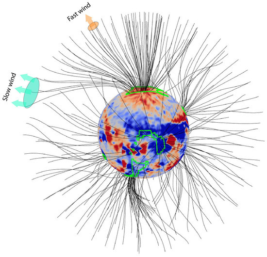
Figure 1.
Demonstration of the WSA model: fast and slow flows. Calculations in the PFSS approximation from the STOP (Kislovodsk Mountain Astronomical Station) observations, 2259 Carrington rotations. The green contours indicate the boundaries of CHs.
Wang and Sheeley [2] investigated this dependence based on Mount Wilson observational data from 1967 to 1988. They used the flux tube expansion (FTE) as a measure of the expansion of open magnetic tubes:
where and are the radial components of the magnetic field at the source surface and the base of the magnetic tube on the photosphere. Wang and Sheeley empirically established a relation between the FTE and the SW velocity at the source surface. Later, the relation was strengthened by another parameter —the great circle distance from the base of the magnetic tube on the photosphere to the boundary of the corresponding CH (DCHB) [3]. Thus, in its modern form, the Wang–Sheeley–Arge (WSA) model is an empirically found dependence of the SW radial velocity component at the source surface on two coronal magnetic field parameters:
where are constant coefficients.
The WSA model is recognized and widely used in problems of modeling SW and space weather forecasting; however, it is not without drawbacks. In some periods, the model may show close to zero or even a negative correlation with the observations [4,5]. Another significant drawback, in our opinion, is that the SW velocity is determined only by the topology of the photospheric magnetic field without taking into account the magnitude. At the same time, FTE cannot be called a universal parameter, although it is the main one in the WSA model. The one parameter dependence of SW velocity on FTE deteriorates with changes in the phase of the solar cycle [6]. The FTE shows a good correlation with high-velocity SW fluxes, but not with slow ones [7]. In a study of SW velocity in pseudostreamers, a statistically significant correlation between observed SW velocity and FTE was not found [8]. It has been proposed to use other magnetic field parameters besides the FTE to model the SW. As an example of the possible parameter responsible for plasma acceleration, the radial component of the magnetic field near the Sun was considered [9]. In particular, it was suggested that, in addition to the FTE, the values and be used to calculate the SW velocity [10].
Thus, the issue of modeling the SW velocity is still open and is actively discussed. Our work is devoted to the search for relationships between various coronal magnetic field parameters and the observed SW velocity, and to constructing a SW model as an alternative to the WSA.
2. Materials and Methods
The calculations of the magnetic field parameters in the present work are based on three data series:
- Solar Telescope-magnetograph for Operative Prognoses (STOP), Kislovodsk Mountain Astronomical Station (KMAS) [11,12]. We used 720 × 360 resolution synoptic maps for 2152–2257 Carrington rotations (CRs) (2014–2022);
- Helioseismic and Magnetic Imager (SDO/HMI) line-of-sight (LOS) magnetic field component synoptic maps at 720 × 360 resolution for 2098–2257 CRs (2010–2022);
- Wilcox Solar Observatory (WSO) magnetic field synoptic maps of 1642–2257 CRs (1974–2022).
Our comparisons of WSA calculations for these data series over different periods can be found in [5]. For the synoptic maps, the pole-filling procedure (in the case of STOP and HMI) and the polar correction were performed. The polar correction, i.e., recalculation of the LOS component into the radial one, was performed by dividing by the sine of the latitude.
To simulate the magnetic field in the solar corona, we used the PFSS approximation by considering the source surface radius and using 15 harmonics. All magnetic field parameters at the source surface were calculated in steps of . At the first stage of the calculations, open field lines were traced from the entire source surface down to the photosphere, and CHs were determined (Figure 1). Then, parameters , , and some others were calculated on the source surface in the ecliptic plane:
- L—length of the open field lines between the photosphere and the source surface in units of the solar radius. In our case, 1.5–3. Assuming that the plasma moves along the field lines, elongation of the field lines will lead to an increase in the influence of the tangential component of the magnetic field on the acceleration of the SW. Thus, we assume that longer field lines should correspond to a slower SW;
- —average angle of deviation of the force lines from the radial direction at different altitude ranges measured in degrees. This parameter is also directly related to the tangential component of the magnetic field;
- —the great circle angular distance to the heliospheric current sheet (HCS) on the source surface measured in degrees. Somewhat indirectly, the dependence of SW speed on the distance to the HCS is also assumed in the WSA model. As one approaches the HCS, tends to zero, and the increases and tends to infinity. Experimentally, the relationship between SW speed and distance to the HCS is confirmed, for example, by observations of Ulysses [13];
- and —absolute values of the radial components of the magnetic field at the source surface and the base of the magnetic field line on the photosphere, measured in Gauss;
- —the latitude of the footpoint of the force line on the photosphere in degrees, zero corresponds to the equator. It is known that the sources of high-speed SW streams observed on Earth are low-latitude CHs [14]. Therefore, it is possible that latitude may be an important parameter.
Data from the OMNIWeb database [15] were used to compare the aforementioned parameters with the observed SW speed. To partially exclude the influence of the CMEs, we did not use data after X- and M-class flares in the comparison. For the propagation of the SW from the source surface to the Earth’s orbit, the ballistic approximation is a popular solution. A description of this method can be found in [16]. We need to do the reverse procedure: compare the measured SW velocity to the parameters of the magnetic field on the source surface. The ballistic model can be very simply reversed by adding a time shift to the series of SW velocity observations. We determine the magnitude of the shift for each measured velocity value individually by dividing the distance from the source surface to 1 AU by the SW velocity. It is important to note that our approach is not an exact inversion of the ballistic model because it does not account for fast SW fluxes. After subtracting the time shift, we interpolated a series of SW velocity data to a regular grid corresponding to the calculated magnetic field parameters (Figure 2). We made calculations on a grid with steps of 2.5 degrees of longitude, which corresponded to about 4.5 h. In the present work, these data with steps of 4.5 h are used only to illustrate the dependence of SW speed on various parameters. For the quantitative analysis, we average the magnetic-field parameters and the SW speed by CR. This allows us to ignore the fluctuations during SW propagation.
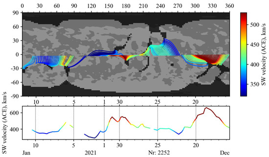
Figure 2.
Open field lines in the ecliptic plane, calculated from magnetograph STOP data, 2252 CR (top panel). The dark regions correspond to the CHs, while the gray and light gray areas depict the different polarities of the photospheric field. The corresponding SW velocity according to the ACE data (bottom panel).
3. Results
The comparison of different combinations of the field parameters with the SW velocity is shown in Figure 3; the images are smoothed by a window with a radius of 1 pixel. First of all, we see how the dependence underlying the WSA model is fulfilled (Figure 3a). The central regions of the CHs correspond to the small FTE and are the sources of fast SW (red and orange pixels). The slow fluxes (blue and green pixels) are observed closer to the edges of the CHs and correspond mainly to large FTE values.
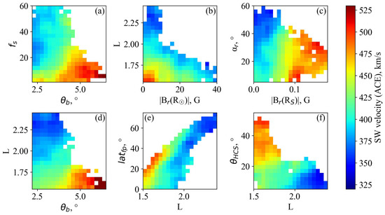
Figure 3.
Relationships between different pairs of magnetic field parameters calculated from magnetograph STOP data (2014–2022) and observed SW velocity V according to the ACE data: (a) ; (b) ; (c) ; (d) ; (e) ; (f) .
From Figure 3 we see that the SW velocity can, in general, be described by various two-parameter dependencies. We can clearly see regions of conditionally high velocities (>450 km/s, red and yellow pixels), medium velocities (400–450 km/s, light blue, and green pixels), and low velocities (<400 km/s, blue pixels). Each region corresponds to a certain range of magnetic field parameter values. Comparing Figure 3a,d, we can see that the character of the dependence of the SW velocity on the line length L is similar to the character of the SW velocity dependence on the FTE. Longer field lines, whose bases lie mainly at high latitudes, bring weak winds to the ecliptic plane. At the same time, the sources of the fastest SW flows are mid-latitude CHs (15–35 latitude, Figure 3e).
We also see a number of other patterns:
- A smaller magnetic field strength at the base of the tube leads to faster winds at the source surface (Figure 3b);
- A higher magnetic field strength at the source surface corresponds, in general, to relatively fast winds (Figure 3c);
- Fast SW fluxes are observed in tubes that deviate, on average, not very much from the radial direction, within (Figure 3c);
- In regions of the source surface strongly distant from the HCS, fast SW is observed and vice versa (Figure 3f).
To find out which parameters are preferable to be used in the SW model, we investigated the correlation of each of the parameters separately with the observed SW velocity. The correlation coefficient was calculated using the values averaged over the CR. By applying averaging, we pursue two goals. First, we initially try to establish the most general correlations between magnetic field parameters and SW. Second, we level out possible inaccuracies associated with applying a ballistic model to the backward propagation of the observed SW. The correlation coefficients for each data series are presented in Table 1.

Table 1.
Pearson correlation coefficients between magnetic field parameters and SW velocity according to CR averaged values.
Judging by the correlation coefficients presented in Table 1, different parameters are preferred for different instruments. However, (DCHB), the second parameter of the WSA model, shows the best performance. Some others also look promising: line length L, great circle distance to the HCS , and . Rather unexpectedly for us, the conclusion is that the FTE turns out to be one of the worst parameters among those considered. A natural question arises: how successful is it possible to simulate the SW velocity without using FTE. Below are examples of the relations constructed from the WSO data on three magnetic field parameters , L, and :
The coefficients in relations (3) and (4) were determined by fitting them to the observed SW velocities . To minimize the differences between the values of and , , the Nelder–Mead method was used. To compare relations (3) and (4) with the WSA model, the same optimization procedure was performed for the WSA model coefficients (2):
4. Discussion
The correlation coefficients in Table 1 vary markedly from instrument to instrument. This is probably due to the different sensitivity of the instruments to weak large-scale fields. Noticeable differences between the instruments also appear in the simulation of open flux, and the simulation based on STOP data is more correct compared to HMI and WSO [17]. According to our calculations (Table 1), the parameter DCHB plays the main role in the WSA model. At large periods, the correlation between the FTE and the SW velocity is close to zero. Optimization of the WSA model coefficients on the data for 2000–2022 leads to the minimization of the FTE contribution (5). Practically, this means that the FTE can be excluded from the WSA model without any noticeable consequences (Figure 4). The WSA model based only on the DCHB (3) is generally correct in describing velocity changes. The model performs worst in the weak SW phases: 2009–2010, 2012–2014, and 2019–2020. This problem is partially solved by adding to the model (as an input parameter) the lengths of field force lines (4), (Figure 5). However, some significant errors, especially in the period 2012–2014, remain. This is probably due to a polarity reversal of the large-scale magnetic field in this period.
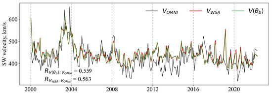
Figure 4.
Example of a single-parameter dependence of the SW velocity ; comparison with the observed velocity and with the velocity calculated according to the WSA model . Calculations using the CR-averaged parameters.
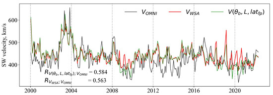
Figure 5.
An example of a three-parameter dependence of SW velocity comparison with the observed velocity and with the velocity calculated according to the WSA model . Calculations using the CR-averaged parameters.
The FTE calculated from the nearly fifty-year WSO data series does not correlate with SW velocity. However, if we consider only conventionally fast SW fluxes (>420 km/s, Table 1), some positive correlation appears. This is similar to the conclusion [7] that FTE correlates better with fast SW fluxes. The generally weak relationship between FTE and SW velocity appears to suggest that FTE is an indirect index that does not determine SW acceleration mechanisms. Such assumptions have been made before, in particular, in the study [8] based on the analysis of velocities in pseudostreamers. However, our result is based on a more general analysis of the SW velocity in the entire ecliptic plane over a long period.
The patterns of correlations between the SW velocity and magnetic field parameters, which we see, among others, in Figure 3, do not contradict the results of other studies. The force-lines length and the average angle of deviation from the radial direction characterize the curvatures of the force lines, which, as studies have shown [18], can lead to a slowing of the SW. The correlation between the lengths of the force lines and the SW velocity that we found does not contradict the results obtained on the basis of MHD modeling [7]. We propose an empirical relationship for calculating the SW velocity based on the DCHB, the lengths of the force lines, and the latitude of the force line footpoints (4). This relationship works slightly better than the WSA model (Figure 5): the correlation coefficient with observations is 0.584 versus 0.563. However, it retains the feature of the WSA model that the results depend only on the topology of the large-scale magnetic field in the photosphere. Perhaps our result can be improved by adding to the model the magnitude of the magnetic field strength at the photosphere and/or at the source surface. A sufficiently high correlation of the with the SW velocity (Table 1) gives hope for this.
Author Contributions
Conceptualization, A.T.; methodology, A.T. and I.B.; software, A.T. and I.B.; validation, I.B.; formal analysis, I.B.; investigation, A.T. and I.B.; writing—original draft preparation, I.B.; writing—review and editing, A.T.; visualization, I.B. All authors have read and agreed to the published version of the manuscript.
Funding
This research was funded by the Ministry of Science and Higher Education of the Russian Federation, grant number 075-03-2022-119/1.
Informed Consent Statement
Not applicable.
Data Availability Statement
The data presented in this study are available in [15].
Conflicts of Interest
The authors declare no conflict of interest.
References
- Levine, R.H.; Altschuler, M.D.; Harvey, J.W.T. Solar Sources of the Interplanetary Magnetic Field and Solar Wind. J. Geophys. Res. 1997, 82, 1061–1065. [Google Scholar] [CrossRef]
- Wang, Y.-M.; Sheeley, N.R., Jr. Solar Wind Speed and Coronal Flux-Tube Expansion. Astrophys. J. 1990, 355, 726. [Google Scholar] [CrossRef]
- Arge, C.N.; Luhmann, J.G.; Odstrcil, D.; Schrijver, C.J.; Li, Y. Stream Structure and Coronal Sources of the Solar Wind during the May 12th, 1997 CME. J. Atmos. Sol.-Terr. Phys. 2004, 66, 1295–1309. [Google Scholar] [CrossRef]
- Poduval, B. Controlling Influence of Magnetic Field on Solar Wind Outflow: An Investigation Using Current Sheet Source Surface Model. Astrophys. J. 2016, 827, L6. [Google Scholar] [CrossRef]
- Berezin, I.A.; Tlatov, A.G. Comparative Analysis of Terrestrial and Satellite Observations of Photospheric Magnetic Field in an Appendix to Simulation of Parameters of Coronal Holes and Solar Wind. Geomagn. Aeron. 2020, 60, 872–875. [Google Scholar] [CrossRef]
- Obridko, V.N.; Kharshiladze, A.F.; Shelting, B.D. On calculating the solar wind parameters from the solar magnetic field data. Astron. Astrophys. Trans. 1996, 11, 65–79. [Google Scholar] [CrossRef]
- Pinto, R.F.; Brun, A.S.; Rouillard, A.P. Flux-tube geometry and solar wind speed during an activity cycle. Astron. Astrophys. 2016, 592, A65. [Google Scholar] [CrossRef]
- Wallace, S.; Arge, C.N.; Viall, N.; Pihlström, Y. On the Relationship between Magnetic Expansion Factor and Observed Speed of the Solar Wind from Coronal Pseudostreamers. Astrophys. J. 2020, 898, 78. [Google Scholar] [CrossRef]
- Rudenko, G.V.; Fainshtein, V.G. Parametric study of interaction effects of fast and slow co-rotating solar wind streams. Planet. Space Sci. 1994, 42, 27–40. [Google Scholar] [CrossRef]
- Belov, A.V.; Obridko, V.N.; Shelting, B.D. Correlation between the Near-Earth Solar Wind Parameters and the Source Surface Magnetic Field. Geomagn. Aeron. 2006, 46, 430–437. [Google Scholar] [CrossRef]
- Tlatov, A.G.; Dormidontov, D.V.; Kirpichev, R.V.; Pashchenko, M.P.; Shramko, A.D.; Peshcherov, V.S.; Grigoryev, V.M.; Demidov, M.L.; Svidskii, P.M. Study of Some Characteristics of Large-Scale Solar Magnetic Fields during the Global Field Polarity Reversal According to Observations at the Telescope-Magnetograph Kislovodsk Observatory. Geomagn. Aeron. 2015, 55, 969–975. [Google Scholar] [CrossRef]
- Kislovodsk Mountain Astronomical Station. Available online: http://solarstation.ru (accessed on 1 October 2022).
- Phillips, J.L.; Balogh, A.; Bame, S.J.; Goldstein, B.E.; Gosling, J.T.; Hoeksema, J.T.; McComas, D.J.; Neugebauer, M.; Sheeley, N.R., Jr.; Wang, Y.-M. Ulysses at 50° South: Constant Immersion in the High-Speed Solar Wind. Geophys. Res. Lett. 1994, 21, 1105–1108. [Google Scholar] [CrossRef]
- Sheeley, N.R., Jr.; Harvey, J.W. Coronal Holes, Solar Wind Streams, and Geomagnetic Activity during the New Sunspot Cycle. Sol. Phys. 1978, 59, 159–173. [Google Scholar] [CrossRef]
- OMNIWeb Plus. Available online: https://omniweb.gsfc.nasa.gov (accessed on 1 October 2022).
- Arge, C.N.; Pizzo, V.J. Improvement in the Prediction of Solar Wind Conditions Using Near-Real Time Solar Magnetic Field Updates. J. Geophys. Res. 2000, 105, 10465–10480. [Google Scholar] [CrossRef]
- Wang, Y.-M.; Ulrich, R.K.; Harvey, J.W. Magnetograph Saturation and the Open Flux Problem. Astrophys. J. 2022, 926, 113–127. [Google Scholar] [CrossRef]
- Li, B.; Xia, L.D.; Chen, Y. Solar winds along curved magnetic field lines. Astron. Astrophys. 2011, 529, A148. [Google Scholar] [CrossRef]
Publisher’s Note: MDPI stays neutral with regard to jurisdictional claims in published maps and institutional affiliations. |
© 2022 by the authors. Licensee MDPI, Basel, Switzerland. This article is an open access article distributed under the terms and conditions of the Creative Commons Attribution (CC BY) license (https://creativecommons.org/licenses/by/4.0/).