Abstract
Complexity is a typical feature of space plasmas that may involve the formation of multiscale coherent magnetic and plasma structures. The winding features (pseudo-polarization) of magnetic field fluctuations at different spatial scales are a useful quantity in this framework for investigating complexity in space plasma. Indeed, a strong link between pseudo-polarization, magnetic/plasma structures, turbulence and dissipation exists. We present some preliminary results on the link between the polarization of the magnetic field fluctuations and the structure of field-aligned currents in the high-latitude ionosphere. This study is based on high-resolution (50 Hz) magnetic field data collected on board the European Space Agency Swarm constellation. The results show the existence of a clear link between the multiscale coarse-grained structure of pseudo-polarization and intensity of the field-aligned currents, supporting the recent findings according to which turbulence may be capable of generating multiscale filamentary current structures in the auroral ionosphere. This feature is also examined theoretically, along with its significance for the rate of energy deposition and heating in the polar regions.
1. Introduction
Dynamical complexity is a quite common feature of solar, interplanetary, and geospace plasmas. The occurrence of chaos, turbulence, and the emergence of multiscale coherent magnetic and plasma structures, whose evolution controls the dynamics of the entire plasma system is one manifestation of dynamical complexity.
In the framework of geospace plasmas, the high-latitude ionosphere is an excellent laboratory to study dynamical complexity and turbulence in strongly magnetized [1,2] and low beta () plasma. This implies a strong anisotropy of the magnetic field turbulent fluctuations that are generally damped along the field direction [3]. In other words, turbulent fluctuations are essentially confined in a plane perpendicular to the magnetic field direction, implying that we are dealing with a two-dimensional (2D) turbulence. Furthermore, the observed magnetic field turbulent fluctuations in the auroral regions are most likely caused by the sporadic fast interactions between localized coherent plasma structures [4,5]. These (see e.g., [6] and references therein) can take the shape of multiscale field-aligned coherent structures (e.g., flux-tubes).
A reasonable approximation to model the turbulent fluctuations in the above scenario is the Reduced Magneto-Hydro-Dynamics (RMHD) (refer to [3]). According to this approximation, the main magnetic field can be described in terms of a constant magnetic field component, , and a flux function , i.e.,
where is the unit vector along the direction. In such a configuration, the current density, , is completely determined by the flux function , being .
In a recent work, Consolini et al. [6] investigated the scaling features of magnetic field fluctuations at high-latitude ionospheric regions where field-aligned currents (FACs) flow, and showed that intermittent turbulence [4] is characteristic of the observed fluctuations. Furthermore, they found that the anomalous scaling features of magnetic field fluctuations perpendicular to the main field can suggest an inhomogeneous and filamentary multiscale structure of FACs.
By assuming that the FACs structure consists of a set of multiscale upward/downward current filaments, the magnetic field components perpendicular to the main magnetic field may consist of multiscale circularly polarized wavelike structures. If we consider the magnetic helicity
where is a volume and is the magnetic vector potential. For a circularly polarized magnetic field in a slab geometry, can be viewed as a measure of the polarization of the wavelike field [7]. In the case of a circularly polarized wave, which is force-free, the associated current density (where k is the wavenumber). Thus, a nonvanishing magnetic helicity is connected to currents flowing along helical magnetic field lines [8]. Consistently, a complex topology of the FACs could be related with a non-zero value of magnetic helicity and, for a turbulent plasma medium, with a non-trivial (power-law) magnetic helicity spectrum, [9,10]. Anyway, the estimation of magnetic helicity from single point measurements is not accessible, this quantity being a volume property. Matthaeus and Smith [11] and Smith [9] showed that in the case of in situ single point measurements it is possible to get statistical information by defining a reduced magnetic helicity, , along the plasma flux direction. Clearly, the generalization of this quantity to different situations such as, for instance, when observations are performed not along the flux direction but in a perpendicular direction, is not trivial. In this case, an alternative way to get a measure of the polarization of a wavelike field is through the use a different approach, such as that discussed in Gedalin and Russel [12]. However, given a fluctuating magnetic field (as, for instance, the case of a turbulent magnetic field) since the corresponding magnetic helicity is
where is the fluctuating part of the magnetic field and the vector potential (), it can be proven that in the Fourier space magnetic helicity is linked to the polarization of the Fourier component , and, in particular, that a circularly polarized has a maximal magnetic helicity [10]. In this framework, the study of polarization of magnetic field fluctuations at different wavenumbers can provide information on magnetic helicity.
Here, we investigate the multiscale features of magnetic field fluctuations by using a method based on the analysis of a pseudo-polarization spectrum (see next Section) during a crossing of the polar ionosphere by the ESA’s Swarm constellation, looking for a possible link with the FACs. We also try an indirect evaluation of the reduced magnetic helicity in the direction perpendicular to that of the main geomagnetic field using the corresponding polarization helicity parallel to the main geomagnetic direction. The aim is to show the multiscale and filamentary character of FACs and its link with the turbulent nature of the ionospheric plasma. We point out that understanding this relationship is crucial for accurately estimating the rate of energy deposition during Space Weather events. Turbulence may imply the formation of complex multiscale current patterns which influence how energy is deposited in the auroral regions during Space Weather events such as magnetospheric substorms.
2. Theoretical Background
In 1998 Gedalin and Russel [12] proposed a method based on wavelet transform to investigate the local polarization spectrum of a wave field that can be applied in our case to get information on the fine structure of the magnetic field fluctuations in the polar ionosphere.
Let us consider a plane wave with wave vector and angular frequency , where is an unit vector with components in a generic plane perpendicular to the direction and the wave amplitude. Then, in the case of a magnetic field, i.e., , as a consequence of the Maxwell equations we have,
i.e., the propagation direction is perpendicular to the phase plane.
In the case of an elliptically (circularly) polarized wave, the field vector rotates within it. This means that we can write the plane wave as a complex wave (see Figure 1), where
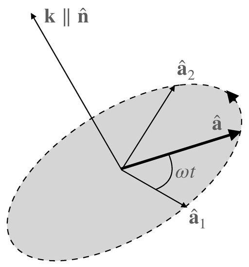
Figure 1.
A schematic picture of the orientation of the vector and the propagation direction in the case of a plane wave.
According to this notation, the circular polarization degree can be written
where . In the case of a non zero circular polarization, , (sometimes referred to as helicity) then it is possible to identify the wave propagation direction, which is given by the expression,
where .
According to Gedalin and Russel [12], the wavelet transform can be applied to Equation (7) so as to obtain a polarization scalogram where is the location and the scale. In detail, if is the magnetic field vector and is the corresponding wavelet transform, where , then one can interpret as a local magnetic field monochromatic wave with and . Consequently, the circular polarization can be computed using the following relation
Analogously, the associated wave propagation direction can be written as
As noted by Gedalin and Russel [12], because the wavelet transform is inherently elliptically polarized, the corresponding degree of linear polarization, , can be estimated using the expression . Furthermore, it is also possible to compute the so called ellipticity , which is defined
where, in the case of magnetic waves, is the component of perpendicular to the plane , while is the component in the plane (see Gedalin and Russel [12]).
In this work, to compute the wavelet transform we use as mother wavelet the complex-valued Morlet wavelet
where is the timescale, a is a constant which controls the exponential decay of the wavelet and N is a normalization factor chosen as to be a square integrable Lebesgue L-function, i.e.,
The L normalization ensures a correct estimation of the power spectrum. Furthermore, we choose and with .
Although this method was originally designed to study the wave polarization, it can be also successfully applied to the crossing of static structures. Indeed, the satellite crossing of a static structure (i.e., evolving on scales larger than the analyzed ones), such as a flux tube and/or a flux rope, will return as a temporal signal similar to a temporal fluctuation associated with a wave. In this instance, we are not dealing with a real polarization, but rather with information on the winding (helical) features of the magnetic field lines. We remark that similar approaches have been applied to study large-scale flux tubes and flux ropes in the solar wind (e.g., [13]). In what follows, when referring to pseudo-static structures, we will use the term polarization exactly with the above mentioned meaning. In other words, we use the described polarization-based method to draw insights into the complex, multiscale nature of the observed spatial fluctuations.
3. Data Description and Methods
We use in situ magnetic field measurements made on board one of the satellite of the ESA Swarm constellation during a crossing of the Northern polar ionosphere [6].
The ESA-Swarm constellation consists of three satellites (A, B, and C), equipped with the same instrumentation, and flying at two different altitudes: 460 km (satellites A and C) and 520 km (satellite B). In this work, we present a preliminary analysis of the possible link between magnetic field polarization and FACs, thus we considered only one of them, Swarm A. Data used refer to Level 1b high-resolution (50 Hz) magnetic field measurements recorded on 25 October 2016, from 17:50 UT to 18:08 UT, a time interval of high geomagnetic activity level (AE nT) already used in a previous work by Consolini et al. [6]. Data are provided in the North-East-Center (NEC) reference frame.
For the same time interval we consider also the FAC density data, a Swarm Level 2 (L2-FAC) single spacecraft product computed from the spatial gradients of the magnetic field along the satellite orbit [14] which are available at ftp://swarm-diss.eo.esa.int (accessed on 31 May 2021) ( file type). Time resolution of FAC data is 1 s.
In order to study the perturbation field associated with FACs in the direction perpendicular to the main geomagnetic field, as a first step, we removed the contribution coming from the main geomagnetic field of internal origin (core and crust) using CHAOS model by Finaly et al. [15]. Thus, we obtain the observed geomagnetic field of external origin. Moreover, the NEC reference frame is not the best one to study the correlation between the polarization and FACs, so we rotated the external magnetic field measurements in a new local frame with axes parallel and perpendicular to the local main geomagnetic field (i.e., essentially the geomagnetic field of internal origin ). In this new local reference frame, the perpendicular components to the main geomagnetic field are chosen so to be almost along the North () and East () components.
Figure 2 shows the components of the magnetic field of external origin parallel and perpendicular to the local main geomagnetic field direction in comparison with those in the NEC reference frame.
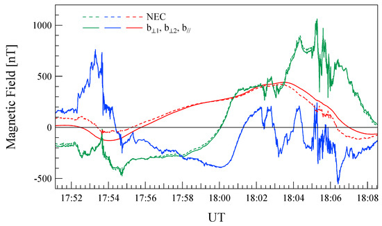
Figure 2.
The external magnetic field components in the NEC reference frame and parallel () and perpendicular () to the local main geomagnetic field. Data refer to measurements recorded on October 25, 2016 from 17:50 UT to 18:08 UT.
The evaluation of fluctuation polarization features is performed according to Equation (8), using as mother-wavelet the Morlet wavelet (see Equation (11)). We investigate timescales s. This interval of timescales has been chosen so to remove the possible instrumental effects (see, e.g., Ref. [6]). Assuming that Taylor’s hypothesis is valid, i.e., where f is the inverse of the timescale and is the spacecraft velocity, i.e., km/s, the considered interval of timescales corresponds to explore the following interval of spatial scales: km. The validity of Taylor’s hypothesis for the investigated timescales has been widely discussed in Consolini et al. [6].
4. Results
As first step we compute the polarization scalogram, , using the three magnetic field components according to Equation (8). Figure 3 shows the scalogram of the circular polarization in the plane time-timescale along with the two magnetic field components perpendicular to the local main geomagnetic field direction.
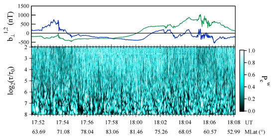
Figure 3.
Upper panel: Magnetic field components, and , perpendicular to the local main magnetic field direction. Lower panel: The scalogram relative to the circular polarization, , with s.
The polarization scalogram exhibits a very complex structure characterized by blobs of circularly polarized fluctuations and linearly polarized ones . In other words, the structure of the polarization is de-facto a coarse-grained multiscale structure. This means that there is not a persistent polarization of the magnetic field fluctuations in the investigated range of timescales.
To investigate the relationship between the circular polarization of the magnetic field fluctuations and FACs, we evaluate the wavelet energy scalogram, , relative to the selected magnetic field time series. Figure 4 shows the obtained results along with FAC density, [14]. A clear correlation between the enhancement of fluctuation energy and is visible.
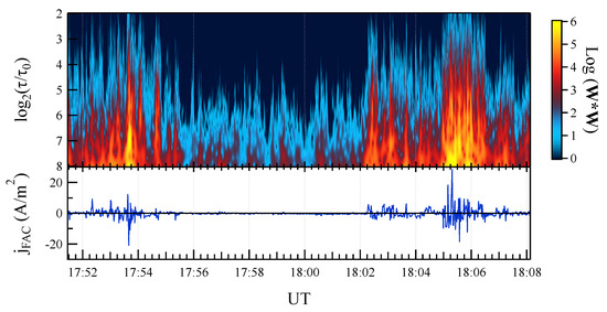
Figure 4.
Upper panel: the wavelet energy scalogram . Lower panel: the FAC density, .
On the basis of the correlation between and the energy scalogram we select two time intervals which allows identifying those regions where the FACs flow: and . We compute the average polarization as a function of the spatial scale in the case of both the entire time series and the two selected FACs intervals.
The obtained results are reported in Figure 5 where the average as a function of the spatial scale for both the entire interval and the selected FAC regions is shown. Circular polarization increases with the decrease of the spatial scale and it is characterized by a larger increase in the case of the analysis performed on the entire interval, especially for km. It is interesting to observe taht at scales greater than 7 km there is no difference in the circular polarization when looking at the entire interval or just FAC regions. The observed features suggest that the main contribution of FACs’ structure to circular polarization is essentially at scales shorter than 7 km. At scales greater than 7 km the similarity may be due to similar magnetic structures, such as macroscale field-aligned coherent flux tubes.
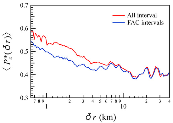
Figure 5.
The average as a function of the spatial scale . Red and blue lines refer to the overall interval and to the two selected FAC intervals, respectively.
As a further step, assuming that the observed polarization structure is related to waves propagating along a specific direction, we compute the component of the propagation direction (see Equation (9)) parallel the main geomagnetic field, i.e., .
Figure 6 shows the scalogram relative to in comparison with . , i.e., the propagation direction is essentially aligned to the main geomagnetic field. Additionally, the sign is not persistent along the different scales, indicating a very complex structure for the propagation direction of fluctuations at different scales. We note that at high latitudes, where FACs do not flow, the short-timescale fluctuations are mainly not parallel to the main geomagnetic field. To better underline the parallel character of the propagation direction of fluctuations, in Figure 7 we show the distribution (PDF) of for a selected number of scales. The distributions are maximal for parallel and anti-parallel directions with respect to the main geomagnetic field. This feature increases with the increase of the spatial scale.
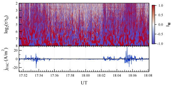
Figure 6.
Upper panel: The component of the propagation direction parallel to the local main geomagnetic field. Lower panel: the FAC density, .

Figure 7.
The probability density function (PDF), , for a selected number of spatial scales, .
We compute the polarization scalogram in the plane perpendicular to the main geomagnetic field due to the very anisotropic nature of the magnetic field fluctuations, which essentially reside in this plane [6]. This quantity is de facto the helicity component, , along the main geomagnetic field (not to be confused with the wavelet ellipticity ) and it is defined as
Figure 8 shows in comparison with . There is not a definite sign of , but conversely the structure of is strongly coarse-grained showing both positive and negative polarization in the plane perpendicular to the main magnetic field. Furthermore, the observed structure of resembles that of suggesting that there should be a correlation between the direction of propagation and the helicity. This correlation is evident if we look at Equations (9) and (13), being proportional to the 3rd component of , i.e., that parallel to the main geomagnetic field, unless of different normalization factor (the denominator). This suggests that the rotation of the magnetic field vector tip in the plane perpendicular to the main geomagnetic field depends on the parallel component of the direction of propagation. This is an extremely interesting point that will help us in the interpretation of the obtained results.
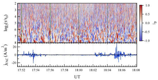
Figure 8.
Upper panel: The polarization scalogram, , in the plane perpendicular to the local main geomagnetic field. Lower panel: the FAC density, .
The last quantity is formally similar to the so-called reduced magnetic helicity [13], being
where, is the reduced magnetic helicity [8,11], is along the plasma flux direction and is in the perpendicular plane. The only difference is that, instead of using as main direction the plasma flux one, , our computation is performed along the satellite orbit which is mainly on a plane perpendicular to the main geomagnetic field, i.e., with .
Following the above-mentioned similitude, we could introduce a quantity similar to by defining
This quantity can be considered as a measure of energy associated with the polarization (in brief: reduced polarization energy) at different scales in the direction perpendicular to the local main geomagnetic field.
Figure 9 shows the scalogram of in comparison with . A large increase of is observed in correspondence with the intensity of FACs which are thus associated with an increase of the amplitude of the helical fluctuations.
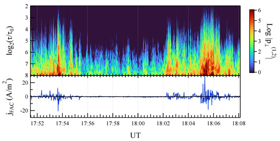
Figure 9.
Upper panel: The scalogram, of , in the plane perpendicular to the local main geomagnetic field. Unit is . Lower panel: the FAC density, .
We report in Figure 10 the average spectra of for the regions where FACs flow and in the polar cap. The spectrum of the reduced polarization energy scales with the spatial scale as
with in the FACs regions.
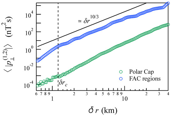
Figure 10.
The average spectra of for the regions where FACs flow and in the polar cap.
The observed scaling reminds that of magnetic helicity observed in the case of homogeneous MHD helical turbulence by Mininni and Pouquet [16], which is observed to scale as (see also [17,18]). This confirms that the reduced polarization energy can provide some insights on the magnetic helicity spectrum. Indeed, according to Stribling et al. [10] in the case of a circularly polarized Fourier component, , the magnetic helicity , so that in terms of power spectral density we have . This means that for a magnetic field characterized by a power law spectral density , the magnetic helicity spectrum is expected to scale as . In our case, as shown in Consolini et al. [6], the magnetic field PSD is characterized by a scaling exponent , so that for the magnetic helicity spectral density the spectral exponent should be , a value which is quite well in agreement with the observed exponent of the reduced polarization energy in the FAC regions. Furthermore, we observe a break in the FAC reduced polarization energy spectrum at a scale of about km, which could be a signature of a new physical process occurring at this scales. This break is not present in the case of polar cap spectrum, which is characterized by a single spectral regime , with .
To disentangle the contribution of positive and negative polarization, we report in Figure 11 the polarization energy associated with negative-hand and positive-hand polarization ( and , respectively). We can see how the structure of the fluctuation field perpendicular to the main geomagnetic field consists of multiscale bundles of fluctuations positively and negatively polarized. There is not an evident asymmetry in the polarization energy distribution between positive and negative polarization in the investigated range of scales km. This suggests that the structure of FACs may consist of a superposition of upward and downward current filaments characterized by different sizes over a wide range of scales.
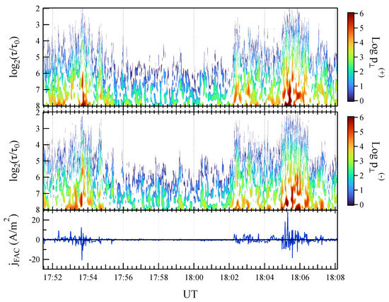
Figure 11.
Upper panel: The scalogram, of positive-hand polarization energy, , in the plane perpendicular to the main geomagnetic field. Mid panel: The scalogram, of negative-hand polarization energy, , in the plane perpendicular to the local main geomagnetic field. Lower panel: the FAC density, . Polarization energy unit is .
5. Discussion
The results of the analyses on the circular polarization of the magnetic fluctuations of external origin described in the previous section, highlight three main outcomes:
- (i)
- circular polarization exhibits a complex multiscale structure especially in regions where FACs flow;
- (ii)
- there is a plane where the magnetic field fluctuations are circularly polarized, that is mainly perpendicular to the local main geomagnetic field direction;
- (iii)
- magnetic fluctuations in the plane perpendicular to the main geomagnetic field consist of multiscale bundles of fluctuations characterized by a positive and negative polarization (helicity ).
Our main results could be interpreted both in terms of a complex current structures consisting of multiscale upward and downward current filaments and in term of a complex multiscale structure of coherent magnetic flux tubes, mainly aligned to the main geomagnetic field and with a different orientation of the magnetic flux (see Ref. [6]), whose dynamics is governed by nonlinear interactions of sporadic and localized coherent structures (see, e.g., [4]). Figure 12 shows a schematic picture of the two possible scenarios involving two different classes of coherent structures: (a) localized currents and (b) coherent magnetic flux tubes.
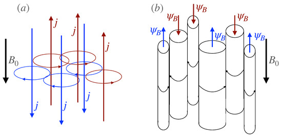
Figure 12.
A schematic picture of the two possible scenarios. Panel (a): a complex current structures consisting of multiscale upward and downward current filaments. Panel (b), a complex multiscale structure of coherent magnetic flux tubes aligned to the main geomagnetic field .
The auroral ionosphere, particularly the region where particle precipitation occurs, is characterized by turbulence phenomena(see, e.g, [6,19,20,21]), as has been extensively discussed in previous works. Since in the polar ionospheric regions the magnetic field is very strong, quasi-uniform, and unidirectional, the fluctuations along the main geomagnetic field direction are damped [3]. We are in a very low beta plasma configuration, i.e., . Thus, magnetic field is essentially potential and the physical scenario can be approximated using the so called Reduced Magneto-Hydro-Dynamics (RMHD) [3].
Recent MHD turbulence simulations (see, e.g, [22,23,24,25,26,27]) have revealed the formation of magnetic field structures aligned to the mean magnetic field on the border of which strong filamentary currents flow. For instance, in Franci et al. [24] it is clear the formation of a complex pattern of field-aligned filamentary current structures due to turbulence. In a recent work, Papini et al. [27] evidenced how currents in turbulent plasmas become increasingly localized, self-organizing in a filamented network at the eddies’ boundaries.
As shown by Greco et al. [23], the presence of internal boundaries between turbulent eddies in space plasmas can be inferred by mean of PVI (partial variance of increments) method, which is based on the estimation of rapid changes in the magnetic field vector, with and is a spatial separation along the satellite trajectory.
Figure 13 shows computed at the smallest available timescale s ( m) in comparison with during the selected time interval. There is an excellent agreement between and supporting the idea that the satellite is crossing a turbulent plasma region characterized by a complex filamented network of currents at the boundaries of field-aligned magnetic structures. Large values of corresponding to the crossing of FAC regions suggest the existence of relevant magnetic discontinuities localized in the regions where currents flow. We point out that the observed discontinuities can be both tangential/rotational and compressional based on definition.
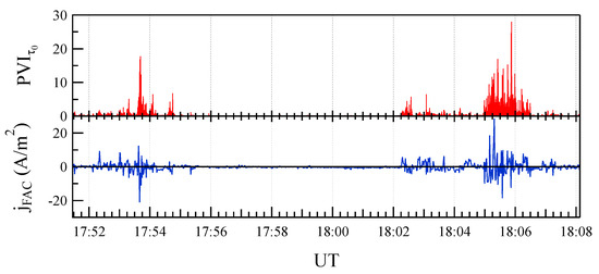
Figure 13.
Comparison between the computed at the smallest available timescale s and the FAC intensity for the selected time interval.
The theoretical emergence of a complex multiscale pattern of polarization, as well as the fractal features of magnetic field fluctuations and FACs [6,28] suggest that the flux function can have a complex structure consisting in the superposition of multiscale flux tubes, assuming as valid the modeling in Equation (1). Indeed, according to the relation between current intensity and the flux function , i.e., , the fractal structure of implies that also the flux fuction has a complex and multiscale structure. In other words, the flux function is a fractal/multifractal scalar field. This scenario is also supported by a previous analysis on the sign-singularity of FACs [28]. Thus, the sign of reported in Figure 6 is associated with the convexity of the magnetic flux-function and, thus, with FAC polarity.
The emerging picture is of a complex multiscale texture of coherent magnetic flux tubes and filamentary currents that are primarily aligned with the main geomagnetic field . Turbulence in the FAC regions could be the cause of such a complex texture. This is supported by simulations of MHD turbulence in low- plasmas with a strong mean magnetic field in a specific direction. It is important to remark that, in this case, magnetic helicity is not conserved since the plasma is non-ideal. Indeed,
where is the electric field and . Here, the last equality follows from the generalized Ohm’s law for a stagnant plasma. The occurrence of dissipation is however expected at the characteristic scales of the current structure. Thus, based on the results plotted in Figure 10 we can speculate that the break observed in the reduced polarization energy is related to the maximal scale associated with the current filaments. In other words, if the scenario of a complex texture of coherent magnetic field structures and filamentary currents is correct the currents should have a size of km.
Another significant point to mention is the effect that a complex current pattern may have on ionospheric plasma heating and energy deposition. Indeed, if the medium where FACs flow is turbulent, the dissipation pattern is expected to be inhomogeneous, particularly in areas where strong currents flow (see, e.g., [23,29]). Since, generally, the dissipation pattern in turbulence has fractal/multifractal features, the estimation of the energy deposition rate and/or the plasma heating based on large scale could be not reliable. Furthermore, as shown in the case of solar wind plasma dynamics, the occurrence of coarse-grained multiscale reconnection and dissipation processes could enhance heating and plasma acceleration [29,30,31]. Indeed, as shown by Tetreault [30], the inherent stochasticity of electric and magnetic field fluctuations associated with a turbulent plasma cannot allow the formation of well-defined flux tubes so that the conservation of magnetic helicity is valid only in a coarse-grained sense (i.e., volume-averaged sense). In such a case, the correct evaluation of dissipation and plasma heating requires taking the topology of the current pattern into account. This is well in agreement with what we have previously discussed.
6. Summary and Conclusions
In this work, we presented a preliminary study of the polarization features of the magnetic field fluctuations at the high-latitude ionospheric regions where FACs flow. Our results evidenced the occurrence of a multiscale complex structure of polarization which is related to the intensity and direction of FACs.
The emerging scenario seems to be consistent with a complex structure of multiscale field-aligned flux tubes as those expected in the case of MHD turbulence in low- plasma with a strong mean magnetic field [24,27]. In this case, currents are expected to be filaments mainly aligned to the mean field direction. The current pattern may be extremely complex and characterized by a fractal topology as it seems to occur in the FAC regions [28]. As a result, the formation of coherent structures and the occurrence of coarse-grained dissipation and heating [30] may imply that a correct evaluation of ionospheric heating must take into account the structure and the dynamics of current pattern. This point is critical for accurately estimating the rate of energy deposition in the high-latitude ionosphere during Space Weather events. Indeed, the emergence of a very complex current pattern as a result of turbulence may imply that a correct estimation of the energy deposited in the auroral ionosphere cannot ignore the small-scale current structure and the occurrence of coarse grained dissipation due to the merging of multiscale magnetic field structures. This specific issue of plasma dissipation and heating in complex fractal pattern will be specifically addressed in a future work in which we will investigate the role of current pattern topology on plasma heating.
Although the above picture is self-consistent and capable of describing the observations, we cannot exclude that other mechanisms, such as, for instance, Alfvén waves and other modes propagating along the mean field direction, could also be relevant to explain some of the previous observations. To disentangle the possible role of waves in generating the observed complex polarization pattern of fluctuations, it is necessary to include other observables (e.g., the electric field and plasma velocity) and to perform other analyses. In this framework, a complementary analysis using ground-based magnetic field measurements from geomagnetic observatories could help to better characterize the FACs dynamics and structure also at lower altitudes. In this case, the use of high-frequency magnetic field measurements (with a temporal resolution higher than 10–50 Hz) would be very useful.
In any case, a better understanding of the observed turbulence processes may benefit from the use of extremely high-resolution measurements, such as those provide by the future NanoMagSat mission [32].
Author Contributions
Conceptualization, G.C. and P.D.M.; methodology, G.C., P.D.M. and T.A.; investigation, G.C., P.D.M. and T.A.; data curation, R.T., I.C., F.G. and M.P.; writing—original draft preparation, G.C., P.D.M. and T.A.; writing—review and editing, all. All authors have read and agreed to the published version of the manuscript.
Funding
This research was supported by the Italian PNRA under Contract PNRA18 00289-A “Space weather in Polar Ionosphere: the Role of Turbulence”.
Data Availability Statement
The results presented relied on data collected by two of the three satellites of the Swarm constellation. We thank the European Space Agency (ESA), which supports the Swarm mission. Swarm data can be accessed online at http://earth.esa.int/swarm (accessed on 31 May 2021).
Acknowledgments
Thanks to the European Space Agency for making Swarm data publicly available.
Conflicts of Interest
The authors declare no conflict of interest.
Abbreviations
The following abbreviations are used in this manuscript:
| 2D | Two-dimensional |
| AE | Auroral Electojet index |
| ESA | European Space Agency |
| FAC | Field-Aligned Current |
| MHD | Magnetohydrodynamics |
| NEC | North-East-Center |
| Probabilty Density Function | |
| PSD | Power Spectral Density |
| PVI | Partial Variance of Increments |
| RMHD | Reduced Magnetohydrodynamics |
| UT | Universal Time |
References
- Kintner, P.M.; Franz, J.; Schuck, P.; Klatt, E. Interferometric coherency determination of wavelength or what are broadband ELF waves? J. Geophys. Res. 2000, 105, 21237–21250. [Google Scholar] [CrossRef]
- Chang, T. Colloid-like Behavior and Topological Phase Transitions in Space Plasmas: Intermittent Low Frequency Turbulence in the Auroral Zone. Phys. Scr. Vol. T 2001, 89, 80–83. [Google Scholar] [CrossRef]
- Biskamp, D. Magnetohydrodynamic Turbulence; Cambridge University Press: Cambridge, UK, 2003. [Google Scholar]
- Chang, T.; Tam, S.W.Y.; Wu, C.C. Complexity induced anisotropic bimodal intermittent turbulence in space plasmas. Phys. Plasmas 2004, 11, 1287–1299. [Google Scholar] [CrossRef]
- Tam, S.W.Y.; Chang, T.; Kintner, P.M.; Klatt, E. Intermittency analyses on the SIERRA measurements of the electric field fluctuations in the auroral zone. Geophys. Res. Lett. 2005, 32, L05109. [Google Scholar] [CrossRef]
- Consolini, G.; De Michelis, P.; Alberti, T.; Giannattasio, F.; Coco, I.; Tozzi, R.; Chang, T.T.S. On the multifractal features of low-frequency magnetic field fluctuations in the field-aligned current ionospheric polar regions: Swarm observations. J. Geophys. Res. Space Phys. 2020, 125, e2019JA027429. [Google Scholar] [CrossRef]
- Moffatt, H.K. Magnetic Field Generation in Electrically Conducting Fluids; Cambridge University Press: Cambridge, UK, 1978. [Google Scholar]
- Matthaeus, W.H.; Goldstein, M.L. Measurement of the rugged invariants of magnetohydrodynamic turbulence in the solar wind. J. Geophys. Res. 1982, 87, 6011–6028. [Google Scholar] [CrossRef]
- Smith, C.W. Magnetic helicity in the solar wind. Adv. Space Res. 2003, 32, 1971–1980. [Google Scholar] [CrossRef]
- Stribling, T.; Matthaeus, W.H.; Oughton, S. Magnetic helicity in magnetohydrodynamic turbulence with a mean magnetic field. Phys. Plasmas 1995, 2, 1437–1452. [Google Scholar] [CrossRef][Green Version]
- Matthaeus, W.H.; Smith, C. Structure of correlation tensors in homogeneous anisotropic turbulence. Phys. Rev. A 1981, 24, 2135–2144. [Google Scholar] [CrossRef]
- Gedalin, M.; Russel, C.T. Application of wavelets to the analysis of multiscale structures. In Physics of Space Plasmas (1998): Proceedings of the 1998 Cambridge Symposium/Workshop in Geospace Physics on Multiscale Phenomena in Space Plasmas II; Chang, T., Jasperse, J.R., Eds.; MIT Center for Theoretical Geo/Cosmo Plasma Physics: Cambridge, MA, USA, 1998; Volume 15, p. 103108. [Google Scholar]
- Telloni, D.; Bruno, R.; D’Amicis, R.; Pietropaolo, E.; Carbone, V. Wavelet Analysis as a Tool to Localize Magnetic and Cross-helicity Events in the Solar Wind. Astrophys. J. 2012, 751, 19. [Google Scholar] [CrossRef]
- Ritter, P.; Lühr, H.; Rauberg, J. Determining field-aligned currents with the Swarm constellation mission. Earth Planets Space 2013, 65, 1285–1294. [Google Scholar] [CrossRef]
- Finlay, C.C.; Olsen, N.; Tøffner-Clausen, L. DTU candidate field models for IGRF-12 and the CHAOS-5 geomagnetic field model. Earth Planets Space 2015, 67, 114. [Google Scholar] [CrossRef]
- Mininni, P.D.; Pouquet, A. Finite dissipation and intermittency in magnetohydrodynamics. Phys. Rev. E 2009, 80, 25401. [Google Scholar] [CrossRef] [PubMed]
- Müller, W.C.; Malapaka, S.K.; Busse, A. Inverse cascade of magnetic helicity in magnetohydrodynamic turbulence. Phys. Rev. E 2012, 85, 15302. [Google Scholar] [CrossRef] [PubMed]
- Müller, W.C.; Malapaka, S.K. Role of helicities for the dynamics of turbulent magnetic fields. Geophys. Astrophys. Fluid Dyn. 2013, 107, 93–100. [Google Scholar] [CrossRef]
- Kintner, P.M.; Seyler, C.E. The status of observations and theory of high latitude ionospheric and magnetospheric plasma turbulence. Space Sci. Rev. 1985, 41, 1572–9672. [Google Scholar] [CrossRef]
- Mounir, H.; Berthelier, A.; Cerisier, J.C.; Lagoutte, D.; Beghin, C. The small-scale turbulent structure of the high latitude ionosphere—Arcad-Aureol-3 observations. Ann. Geophys. 1991, 9, 725–737. [Google Scholar]
- Golovchanskaya, I.V.; Ostapenko, A.A.; Kozelov, B.V. Relationship between the high-latitude electric and magnetic turbulence and the Birkeland field-aligned currents. J. Geophys. Res. (Space Phys.) 2006, 111, A12301. [Google Scholar] [CrossRef]
- Wu, C.C.; Chang, T. 2D MHD simulation of the emergence and merging of coherent structures. Geophys. Res. Lett. 2000, 27, 863–866. [Google Scholar] [CrossRef]
- Greco, A.; Servidio, S.; Matthaeus, W.H.; Dmitruk, P. Intermittent structures and magnetic discontinuities on small scales in MHD simulations and solar wind. Planet. Space Sci. 2010, 58, 1895–1899. [Google Scholar] [CrossRef]
- Franci, L.; Landi, S.; Verdini, A.; Matteini, L.; Hellinger, P. Solar Wind Turbulent Cascade from MHD to Sub-ion Scales: Large-size 3D Hybrid Particle-in-cell Simulations. Astrophys. J. 2018, 853, 26. [Google Scholar] [CrossRef]
- Papini, E.; Franci, L.; Landi, S.; Verdini, A.; Matteini, L.; Hellinger, P. Can Hall Magnetohydrodynamics Explain Plasma Turbulence at Sub-ion Scales? Astrophys. J. 2019, 870, 52. [Google Scholar] [CrossRef]
- Franci, L.; Stawarz, J.E.; Papini, E.; Hellinger, P.; Nakamura, T.; Burgess, D.; Landi, S.; Verdini, A.; Matteini, L.; Ergun, R.; et al. Modeling MMS Observations at the Earth’s Magnetopause with Hybrid Simulations of Alfvénic Turbulence. Astrophys. J. 2020, 898, 175. [Google Scholar] [CrossRef]
- Papini, E.; Cicone, A.; Piersanti, M.; Franci, L.; Hellinger, P.; Landi, S.; Verdini, A. Multidimensional Iterative Filtering: A new approach for investigating plasma turbulence in numerical simulations. J. Plasma Phys. 2020, 86, 871860501. [Google Scholar] [CrossRef]
- Consolini, G.; De Michelis, P.; Coco, I.; Alberti, T.; Marcucci, M.F.; Giannattasio, F.; Tozzi, R. Sign-Singularity Analysis of Field-Aligned Currents in the Ionosphere. Atmosphere 2021, 12, 708. [Google Scholar] [CrossRef]
- Valentini, F.; Perrone, D.; Stabile, S.; Pezzi, O.; Servidio, S.; De Marco, R.; Marcucci, F.; Bruno, R.; Lavraud, B.; De Keyser, J.; et al. Differential kinetic dynamics and heating of ions in the turbulent solar wind. New J. Phys. 2016, 18, 125001. [Google Scholar] [CrossRef]
- Tetreault, D. Turbulent relaxation of magnetic fields 1: Coarse-grained dissipation and reconnection. J. Geophys. Res. 1992, 97, 8531–8540. [Google Scholar] [CrossRef]
- Tetreault, D. Turbulent relaxation of magnetic fields 2. Self-organization and intermittency. J. Geophys. Res. 1992, 97, 8541–8547. [Google Scholar] [CrossRef]
- Hulot, G.; Léger, J.M.; Vigneron, P.; Jager, T.; Bertrand, F.; Coïsson, P.; Deram, P.; Boness, A.; Tomasini, L.; Faure, B. Nanosatellite high-precision magnetic missions enabled by advances in a stand-alone scalar/vector absolute magnetometer. In Proceedings of the IGARSS 2018 IEEE International Geoscience and Remote Sensing Symposium, Valencia, Spain, 22–27 July 2018; pp. 6320–6323. [Google Scholar] [CrossRef]
Publisher’s Note: MDPI stays neutral with regard to jurisdictional claims in published maps and institutional affiliations. |
© 2022 by the authors. Licensee MDPI, Basel, Switzerland. This article is an open access article distributed under the terms and conditions of the Creative Commons Attribution (CC BY) license (https://creativecommons.org/licenses/by/4.0/).