Article

A Correction Algorithm of the Sampling Effect and Its Application in High-Precision Astrometry

1
Department of Physics, Tsinghua University, Beijing 100084, China
2
Xingfan Information Technology Co., Ningbo 315500, China
*
Author to whom correspondence should be addressed.
These authors contributed equally to this work.
Universe 2022, 8(11), 593; https://doi.org/10.3390/universe8110593
Submission received: 20 September 2022 / Revised: 3 November 2022 / Accepted: 5 November 2022 / Published: 11 November 2022
(This article belongs to the Section Space Science)

Abstract

:
The sampling effect of the imaging acquisition device is an integration of the input signal within the pixel, resulting in an additional error in the pixel value. Additionally, a sampler with asymmetric intra-pixel quantum efficiency leads to position errors in high-precision astrometry. This paper proposes a model for the integral sampling process. An algorithm that solves the sampling effect, as well as the position error with high accuracy, is also provided. This algorithm provides an accuracy increase of 10 6 for Gaussian images with a uniform integral sampler. The accuracy limit of the Gaussian image comes from the truncation error. Also, this algorithm provides about 4 times accuracy improvement by eliminating the systematic error caused by the integral sampler with asymmetric intra-pixel quantum efficiency.

1. Introduction

The pursuit of high-precision astrometry is rising three major concerns about modern astronomy, which are the high-precision instruments, the algorithms for astronomical data processing, and the weak signals. Currently, interferometers are the most precise instrument in both optical and radio astronomy. Scholler et al. [1] provided a comprehensive model for the imaging process in stellar interferometers. The algorithms for studying astronomical data are also advancing high-precision astronomy. Ghaderpour [2] developed a least-squares wavelet method for VLBI baseline length analyses. To extract data from the large amount of data provided by various survey missions, Mena et al. [3] put forward a representation using variational auto-encoders for Kepler light curves. Most importantly, signals from faint objects are currently gaining more concentration in the realm of high-precision astrometry. The detection of these objects helps answer some vital questions like learning the nature of dark matter and the cosmos, finding habitable exoplanets, and the state of matter in extreme environments. As Malbet [4] has pointed out, to perform such observations, certain technology challenges must be overcome, including the intra-pixel effects. These works would inspire the development of high-precision astronomy.
The intra-pixel sensitivity variation of the CCD/CMOS chips is the main cause of the intra-pixel effect. To this end, this paper provides a model for describing the sampling process of CCD/CMOS chips, which solves the sampling effect with intra-pixel efficiency variation effectively. The sampling process of most current image sensors is an integration process. This process would cause a deviation between the recorded signal and the input signal, which results in an accuracy loss. The deviation, which would be referred to as the sampling effect, caused by the sampling process is referred to in some studies as part of the total modulation transfer function (MTF) of an image acquisition process and causes the additional blur to the observed images by Fliegel [5], Boreman [6], and Feltz and Karim [7,8].
Despite its initial studies in computer vision, the sampling effect with an asymmetric intra-pixel quantum efficiency (QE) is receiving more concentration recently in astronomical instruments like Kepler, TESS, and JWST (see Lystrup et al. [9], Krishnamurthy et al. [10], Hardy et al. [11] and Hardy et al. [12]). For space telescopes like HST and JWST, the measurement of their CCDs’ intra-pixel sensitivity (IPS) is vital to the position accuracy of their guidance sensor cameras and their infrared detectors (see Robberto et al. [13], Hardy et al. [11] and Hardy et al. [12]). Recent studies in pursuit of high-precision astrometry by Toyozumi and Ashley [14] and Mahato et al. [15] suggest the IPS could cause subtle deviation in the position accuracy. Therefore, the demand for high-precision astrometry urges detailed studies of the integral samplers with intra-pixel sensitivity variation (IPSV).
Currently, there are two major measurement methods of the IPS, one is the interference pattern method based on Fourier Transform (see Ketchazo et al. [16], Willemin et al. [17], and Takacs et al. [18]) and another is the beam spot scanning method (see Toyozumi and Ashley [14], Li et al. [19], and Mahato et al. [20]). These measurements show directly that the IPS varies in different sensors, causing certain defects in both image acquisition accuracy and position accuracy.
To improve the accuracy of image acquisition, researchers proposed several compensation algorithms for the total MTF [21,22,23]. Li et al. [21] proposed a self-compensation method for dynamically inverting the MTF based on multiple natural sub-resolution features, which increases the image quality for remote sensing cameras. These studies provide a perspective to solve the integral sampler’s sampling effect within the frame of the MTF. Still, the demand for high-precision astronomical image analysis urges a recovery algorithm for the integral sample signal for a better understanding of the original signals.
This paper studies the integral sampling effect from a basic image sensor model and gives the direct connection between the impulse sample and the integral sample by the Fourier analysis method. This paper proves that the sampling effect causes an accuracy loss in signal amplitude. For images with appropriate sampling frequency and spatial feature, we put forward a matrix equation for calculating the accurate impulse sample from the integral sample, which decreases the relative error between the recorded signal and the impulse sample by 10 6 . Furthermore, we study the systematic position error caused by the asymmetric intra-pixel sensitivity variation and improve the position accuracy by applying the correction algorithm for the sampling effect.

2. Models for Image Sensors and Sampling Process

The sampling theory and the mathematics for the sampling process are discussed profoundly in recent studies (see Fliegel [5], Boreman [6], Feltz and Karim [7], Vitek and Hozman [24], Park et al. [25]). Based on the current theory, we now introduce a geometric model for an ideal image sensor array. As is shown in Figure 1, a single pixel has a size of 2 L × 2 L , and its photon-sensitive area has a size of 2 ( L d ) × 2 ( L d ) located at its center. And the image sensor array is a duplication of a single pixel.

2.1. Models for Integral Sampling Process

We introduce a model for describing the photon flux distribution on an imaginary plane that coincides with the pixels. We define the optical center of the imaging system as the origin of the coordinate system ( u , v ) on this imaginary plane. Since every single pixel accumulates all the incident photons within its photon-sensitive area, the readout signal I ˜ m n should be proportional to the integral of incident flux I ( u , v ) within the shutter time, which gives the equation for an ideal integral sampling process as Feltz and Karim mentioned [7],
I ˜ m n = e m n I ( u , v ) d u d v ,
where I ˜ m n is the integral flux on the pixel at the mth row and nth column, I ( u , v ) is the photon flux distribution before they reach the sensor, e m n is the shape of the single pixel. We assume the incident flux is time-independent and dismiss the influence of shutter time on the sampler for convenience. Note that this equation has an equivalent convolution form since the pixel’s shape function usually is asymmetric.
We further abstract an integral model before the sensor unit samples the signal. Recall that a typical impulse sampling process is X m n = X ( u = m T , v = n T ) with T representing the sampling interval for a given signal X ( u , v ) . We now consider the I ˜ m n as the impulse sample of a certain continuous signal I ˜ ( u , v ) . The definition of I ˜ ( u , v ) is given directly as,
I ˜ ( u , v ) = e u v I ( s , t ) d s d t ,
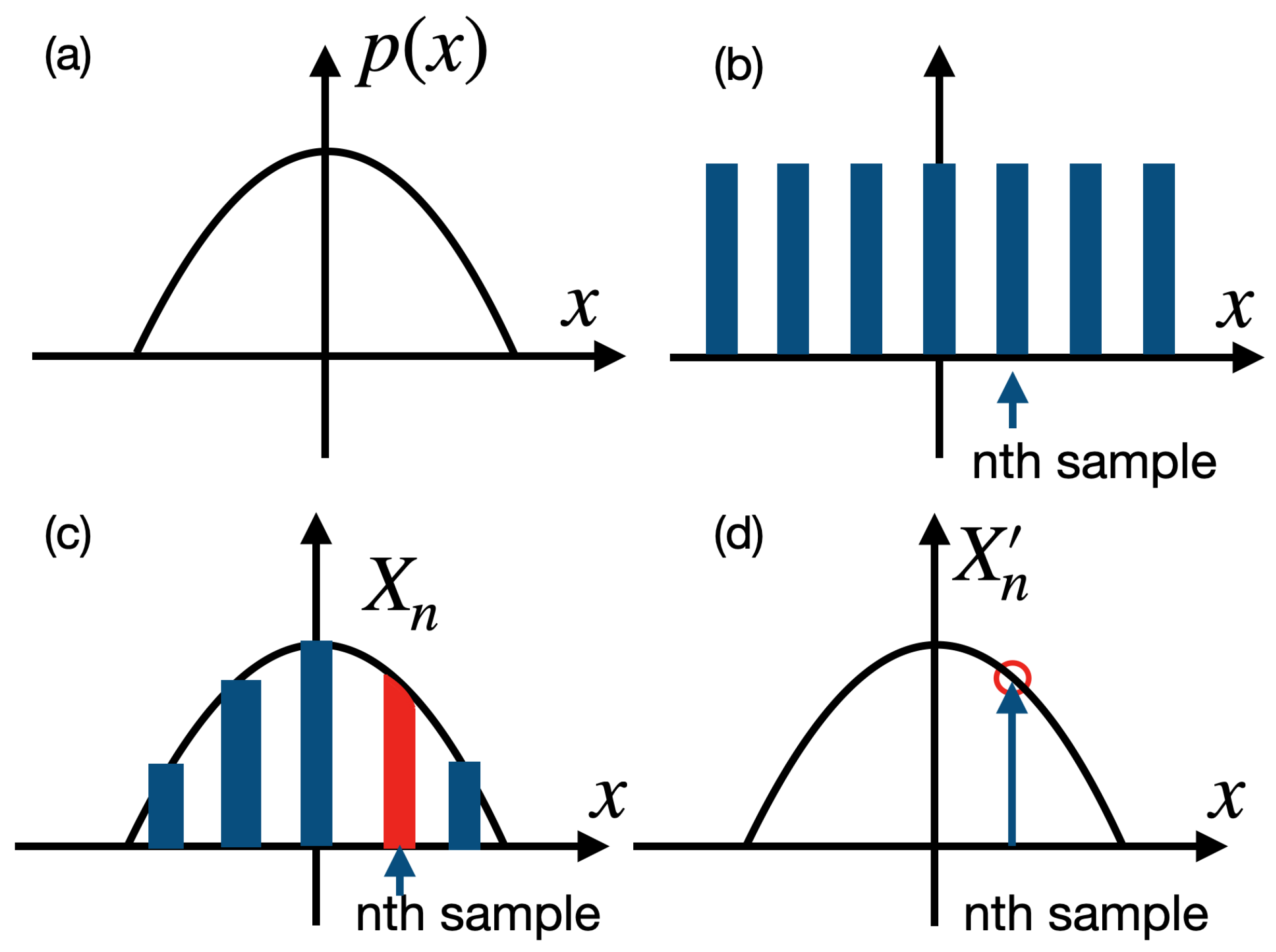
where e u v is an imaginary pixel whose center is located at ( u , v ) . It has an identical shape as the actual pixel e m n . Figure 2 illustrates a one-dimensional sampling effect.
The Shannon Sampling Theorem [26] gives the relation between the impulse signal and its corresponding continuous signal. This can be easily applied to I ( u , v ) and as,
I ( u , v ) = m n I m n sinc ( u m D D ) sinc ( v n D D )
where D is the distance between 2 neighboring sample points. sinc ( x ) = sin ( π x ) / ( π x ) . I ( u , v ) is the flux distribution before being recorded by the sampler array, and I m n is the impulse sample of I ( u , v ) . In the geometric model for the sensor unit, D = 2 L is the length of a single pixel.
Combine Equations (2) and (3) gives the direct connection between the integral sample I ˜ m n and the flux distribution I ( u , v ) , such that,
I ˜ m n = e m n I ( u , v ) d u d v = e m n i j I i j sinc ( v i D D ) sinc ( u j D D ) d u d v = i j I i j e m n sinc ( v i D D ) sinc ( u j D D ) d s d t ,
where the summation and the integration are exchangeable because the integration in Equation (2) is finite within a single pixel. Note that the integration can be calculated directly with any known pixel shape, thus we can define a shape tensor to represent the result of the integration, such that,
S i j m n = e m n sinc ( u j D D ) sinc ( v i D D ) d u d v ,
Then Equation (4) can be simplified and we can write its discrete version directly by substituting ( u , v ) by its sample points ( i , j ) , such that,
I ˜ m n = i j I i j S i j m n .
This equation describes the direct relationship between the impulse sample signal I m n and the integral sample signal I ˜ m n . The integral sample is different from the impulse sample by a shape tensor S i j m n , which is determined by the relative geometric parameters of the pixels.

2.2. Practical Method for Integral Sampling Correction

We provide a practical method for solving the sampling process with a simple geometric pixel structure. Consider a rectangular pixel with a given gap around it. As is shown in Equation (1), the pixel area is ( m D ( L d ) , m D + ( L d ) ) × ( n D ( L d ) , n D + ( L d ) ) . The shape tensor of this rectangle is,
S i j m n R = m D ( L d ) m D + ( L d ) n D ( L d ) n D + ( L d ) sinc ( u j D D ) sinc ( v i D D ) d u d v ,
which is fully determined by the given geometric parameters of the sensor array. We should notice that S i j m n R can be divided into the product of two identical symmetric transferring matrix R with
R m i = m D ( L d ) m D + ( L d ) sinc ( v i D D ) d v ,
and
S i j m n R = R m i R n j .
Then Equation (6) is simply I ˜ m n = i j I i j R m i R n j , or a matrix equation,
I ˜ = R T · I · R .
Suppose the transferring matrix R is invertible. Then we can calculate the impulse sample I i j from the integral sample I ˜ m n , such that,
I = R 1 · I ˜ · R 1 .

2.3. Models for Intra-Pixel Sensitivity and Its Correction Algorithm

The intra-pixel sensitivity is the variation of the QE inside a single pixel. It causes errors in the photon counts and the position accuracy of point sources. A traditional method to fix the intra-pixel QE is to measure the sub-pixel QE and fix the single-pixel QE by dividing its average. However, the influence of the QE deviation on the astrometry remains. With the model and the correction algorithm for the integral sampler, we found a subtle difference between an ideal integral sampler array with uniform QE and with asymmetric QE.
We first build the mathematical model of an asymmetric QE integral sampler array. The imaging process involved with the asymmetric QE is to modify the response inside a single pixel subject to its QE. Suppose that the QE function for the pixel located at the m t h column and the n t h row is Q m n ( u , v ) . Recall the ideal integral sampling equation (Equation (2)), and put the QE function inside. We get the equation for an integral sampling process with arbitrary intra-pixel sensitivity,
I ˜ m n = e m n Q m n ( u , v ) I ( u , v ) d u d v ,
where e m n defines the integral boundary for the pixel located at the m t h column and the n t h row.
We follow the assumptions that the incident ideal signal I ( u , v ) is a band-limited signal and the sampling array meets the Nyquist-Shannon Sampling Theorem. In that case, we substitute I ( u , v ) with its Shannon interpolation, such that,
I ˜ m n = e m n Q m n ( u , v ) ( i j I i j s i n c ( u j ) s i n c ( v i ) ) d u d v ,
where we neglect the gap between pixels and set their length to 1.
However, we cannot define the transferring matrix R as Equation (8) because the unknown QE function may not be separable. Although the precise feature of the QE function remains unknown, it is convenient for us to simulate a CCD array with an asymmetric and separable QE function, such as,
Q m n ( u , v ) = exp ( ( u + u d u m n ) 2 + ( v + v d v m n ) 2 2 σ q 2 ) ,
where u d and v d define the relative center position of a Gaussian function inside the pixel with respect to the pixel’s center ( u m n , v m n ) and σ q describes the profile of the Gaussian QE function. This function can be separated into the product of two individual Gaussian, such that,
Q m n ( u , v ) = exp ( ( u + u d u m n ) 2 2 σ q 2 ) · exp ( ( v + v d v m n ) 2 2 σ q 2 ) .
Then we can define the transferring matrix R and R by swapping the integral and the summation, such that,
R j n = e n exp ( ( u + u d u m n ) 2 2 σ q 2 ) s i n c ( u j ) d u ,
and
R i m = e m exp ( v + v d v m n ) 2 2 σ q 2 s i n c ( v i ) d v ,
where e m and e n denote the corresponding integral boundary.
Therefore, we can conclude a simplified relation between the images recorded by the ideal impulse sampler and the integral sampler with asymmetric QE, such that,
I ˜ m n = i j R i m T I i j R j n ,
or in a matrix equation,
I ˜ = R T · I · R ,
where I ˜ denotes the image recorded by the integral sampler with asymmetric QE, and I denotes the image recorded by an ideal impulse sampler. If both R and R are invertible matrices, we can calculate I by reversing the matrix equation, such that,
I = ( R T ) 1 · I ˜ · R 1 .
Note that this matrix equation is only applicable when the QE function Q m n ( u , v ) is separable. For a complicated Q m n ( u , v ) , we need to calculate the tensor expanded by the integration,
R R i j m n = e m n Q m n ( u , v ) s i n c ( u j ) s i n c ( v i ) d u d v ,
and this problem can also be solved.

2.4. Spatial Frequency Constraints

The application of the Shannon Sampling Theorem into the correction method for the sampling effect gives inherent constraints on the spatial frequency of I ˜ m n . The theorem only treats a band-limited signal with its highest spatial frequency f c smaller than half of the sampling rate of the system f N (see Boreman and Glenn [27]). The Nyquist sampling rate f N of the imaging system is determined by the imaging device and the image sensor, which is f N = 1 / D . For a imaging device with a Gaussian PSF with p ( u , v ) = 1 / ( 2 π σ 2 ) exp ( ( u 2 + v 2 ) / σ 2 ) ) , the spectrum of the PSF is its Fourier Transform P ( U , V ) , which is still a Gaussian distribution with P ( U , V ) = exp ( 2 π 2 σ 2 ( U 2 + V 2 ) ) . For | U | > 5 / ( 2 π σ ) and | V | > 5 / ( 2 π σ ) , we can consider P ( U , V ) 0 . This gives the bandwidth of the Gaussian PSF with f c = 5 / ( 2 π σ ) . The Nyquist Sampling Theorem requires,
f c < f N 2 ,
which is equivalent to
σ D > 5 π ,
note that σ / D is the equivalent standard deviation for a dimensionless imaging system.
To design an imaging system that meets the Nyquist Sampling Theorem, (23) is an essential constraint.

3. Simulations and Applications

To verify the influence of the integral sample and the correction algorithm, we generate a series of simulations and test the correction method on them. The simulation procedure includes the following steps. First, we set a shift-invariant imaging system with a given point spread function. Then we generate the 2-D object, which is a 2-D flux distribution on the object plane. After the imaging system images the 2-D object, we sample the signal by impulse sample method and integral sample method and apply the correction algorithm to the integral sample signal to acquire a signal recovered from the sampling process.

3.1. Reconstructions for Ideal Integral Sampler

We simulate an imaging system that has a Gaussian point spread function (PSF). The sensor unit has a dimensionless size of 1 × 1 (which means D = 1 and d = 0 ), and the PSF of the system is p ( u , v ) = exp ( ( u 2 + v 2 ) / ( 2 σ 2 ) ) with σ = 3 . The ideal image on the object plane consists of two separate Gaussian PSF, such that,
I ( u , v ) = exp ( ( u u 0 ) 2 + ( v v 0 ) 2 2 σ 2 ) + 0.1 · exp ( ( u u 0 u s ) 2 + ( v v 0 v s ) 2 2 σ 2 ) ,
where u 0 = v 0 = 26 , u s = v s = 5 in pixel coordinate. We simulate the imaging process of this system with the given object plane and sample the images by the integral sampler and impulse sampler separately.
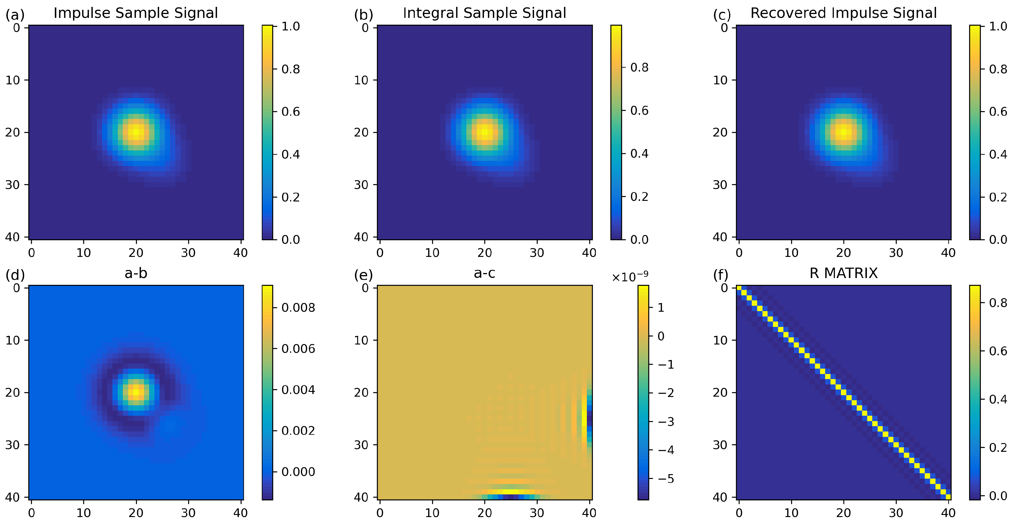
Figure 3 shows the sampled image and the recovered image from the integral sampler. This simulation indicates that the sampling effect from substituting the impulse sampler with an integral sampler can cause significant relative error up to 1 % at the center of the incident flux. By applying the recovery algorithm to the integral sample image, we recover an accurate flux distribution of the two-point sources after the imaging device and reduce the relative error to 10 8 , which is 10 6 better than the integral sample image.
Also, the error image itself shows a fringe pattern at its corner, which is spatially connected to the point source at ( 26 , 26 ) in the image’s coordinate system. This pattern is a Gibbs phenomenon caused by the discontinuous components from the point source at ( 26 , 26 ) , and it contributes the most to the error component in the recovery method.

3.2. Reconstructions for the Integral Sampler with Asymmetric QE

We also simulate the integral sampler with asymmetric QE and prove the correction method in Section 2.3 can improve the position accuracy measurement for a single PSF. The imaging system also has a Gaussian PSF as
I ( u , v ) = 1 2 π σ 2 exp ( ( u u 0 ) 2 + ( v v 0 ) 2 2 σ 2 ) ,
where σ = 2 . The sensor array is 13 × 13 and every pixel has a normalized size with 1 × 1 . The QE distribution in one pixel is,
Q m n ( u , v ) = exp ( ( u + u d u m n ) 2 + ( v + v d v m n ) 2 2 σ q 2 ) ,
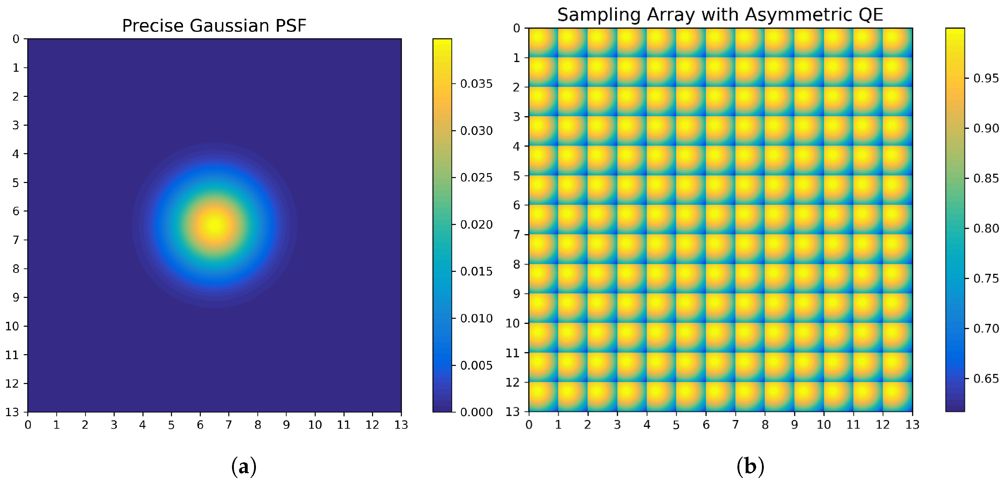
where σ q = 1 and the center of the Gaussian QE function is at ( u m n u d , v m n v d ) . Figure 4 shows the Gaussian PSF and the response to a uniform illumination by the asymmetric QE array. The intra-pixel sensitivity pattern has a clear offset to the top-left corner in every pixel. We would refer to this array as the asymmetric integral array in the following text.
To illustrate the influence of the asymmetric integral array on position accuracy, we sample the PSF with both a uniform integral sampler array and the asymmetric integral array. Figure 5 is the images from the uniform integral sampler array and the asymmetric integral array. From Figure 5c, we can observe slight deformation from the ideal PSF. Besides, since the QE in every pixel is not normalized, the pixel value is smaller than the actual flux integration, which should be fixed by the average QE.
Then we calculate the barycenter of both PSF and compare the results to the ideal centroid on the image plane. If the Gaussian PSF is symmetric, the barycenter of the PSF should be its center. The barycenter calculated by each image is listed in Table 1. From Table 1, we find that the uniform integral sampler has a 7.69 × 10 4 relative error to the ideal PSF center, while the asymmetric integral sampler has a 3.24 × 10 3 relative error.
To fix the relative error caused by the asymmetric integral sampler, we applied the correction method mentioned in Section 2.3. By calculating the transferring matrix R and R , we managed to recover an image recorded by the uniform integral sampler. We compare the image from the asymmetric integral sampler and its recovered image to the original image from a uniform integral sampler and find that the image from the asymmetric integral sampler has obvious deviation in the image plane. Figure 6 shows the direct influence of the asymmetric integral sampler on the position accuracy. In Figure 6b, we observe two separate Gaussian peaks, which means the obvious deviation caused by the asymmetric integral sampler. However, in Figure 6c, we observe a symmetric error pattern similar to those in Figure 3e, which is caused by the truncation error of Shannon’s interpolation.
We also calculate the barycenter of the recovered uniform QE image (Figure 6a) and compare those results to the ideal centroid. In Table 2, we can find that the barycenter calculated by the recovered uniform QE image is rather closer to the ideal centroid compared to that calculated by the asymmetric QE image. Besides, the relative error also reduces to 7.85 × 10 4 .
Since the actual imaging process is a cumulative and statistical process dealing with the ensemble of individual incident photons, we also simulate the influence of the asymmetric integral sampler’s response on randomly distributed photons. Suppose there is a point source that emits 10 5 photons during the integration time. Every photon has a random position ( x p , y p ) on the image plane. The random position ( x p , y p ) follow a normal distribution respectively, which is
x p N ( x r , σ s ) , y p N ( y r , σ s ) ,
where ( x r , y r ) is the ideal position of the point source on the image plane and σ s = 2 . Once we collect all the photons on the image on the image plane, we could claim that we observe the point source. Since the imaging instruments might have slight jittering during the observations, the ideal position of the point source might change randomly in different observations. We assume the ideal position of the point source on the image plane follows a uniform distribution respectively, which is
x r U ( 0.5 , 0.5 ) , y r U ( 0.5 , 0.5 ) .
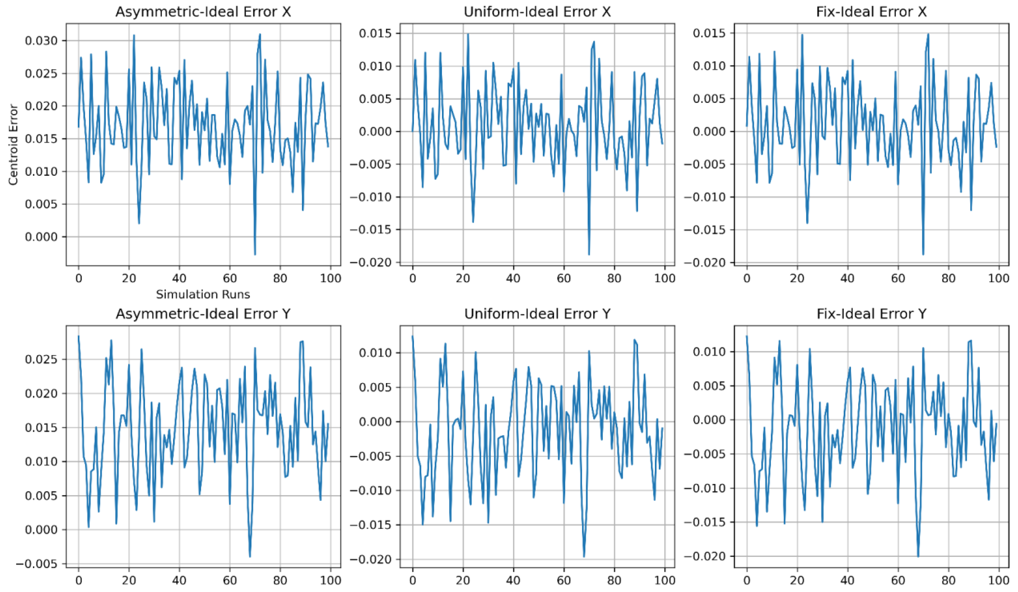
The imaging process is rather straightforward in the tone of collecting individual photons. For every ( x r , y r ) , we record the position of every photon and calculate its response on the integral sampler with the QE function. Then we accumulate the total response to generate an observed image. In contrast to the asymmetric integral sampler, we also make observations with a uniform integral sampler whose QE function is a simple 1. We run the correction algorithm on these observed images and calculate the barycenter of both observed images and their fixed ones. We compare them to the ideal position of the point source to decide whether the systematic error is significant. We collect 100 groups of ( x r , y r ) with their corresponding photon statistical results and calculate their barycenters. The results are listed in Figure 7, and Table 3 and Table 4.
Figure 7 shows there is a clear deviation from observation by the asymmetric integral sampler in both dimensions. In Table 4, we can find that the asymmetric integral sampler reports 0.017 pixel deviation in the x dimension and 0.015 pixel in the y dimension. Both are about 10 times bigger than those deviations calculated by uniform and fixed integral sampler, which is both 0.001 and 0.001 respectively in both dimensions. Meanwhile, the standard error in both tables (Table 3 and Table 4 are relatively close, which indicates they are mainly caused by the distribution of the ideal position of the point source. Therefore, the significant difference in the position calculated by the asymmetric integral sampler from the ideal point position is a systematic error caused by the intra-pixel sensitivity variation, which is specifically related to the asymmetric QE functions we applied here.

4. Discussion

Two key factors determine the improvement of an integral sample signal. One is the spatial frequency response of the imaging system. A PSF that fully meets the Nyquist Sampling Theorem would provide the most accurate result when calculating the shape matrix R . The design of high accuracy imaging system should consider the connection between the imaging device and the image sensor as is discussed in Section 2.4. Figure 8 shows the relation between the relative error and the system’s σ .
Figure 8 also indicates that the demand for high-accuracy imaging systems should focus on producing image sensors with smaller sizes instead of generating imaging devices with smaller PSF. As Section 2.4 discussed, an appropriate σ which is about 2 times the pixel’s length is more appropriate for designing a high-accuracy image acquisition system than a small σ .
The other important factor is the simple fact that the discrete Fourier transform in the algorithm requires the signals to be periodic and continuous at their border. The discontinuous components contribute to the main error in our recovery algorithm, which can be directly spotted from the Gibbs phenomenon in Figure 3 and Figure 6c. To reduce the error induced by the discontinuous components, it might be feasible to apply an additional Gaussian low-pass filter on the integral sampled signal.
The systematic position error caused by the asymmetric integral sampler is vital in high-precision astrometry. For an asymmetric QE function, 0.2 pixel deviation from one pixel’s geometric center would be enough to cause an obvious drift in the image’s barycenter. Since the ideal integral sampler with uniform QE distribution is far too difficult to achieve, recovering an image with a uniform integral sampler from the asymmetric integral sampler provides an easier yet more accurate method for further studies in high-precision astrometry. However, the problems of sampling require more detailed studies into the full working procedure of a sampler. Despite the intra-pixel sensitivity variation, adding other essential factors such as gains and charge transfer inefficiency to the whole sampling model would be the focus of the next studies.

5. Conclusions

This paper discussed the mathematical model for an integral sampler with uniform quantum efficiency and asymmetric quantum efficiency. The relative error caused by the sampling effect relates strongly to the size of the sensor’s unit compared to the PSF’s size. We provided a thorough correction algorithm for imaging systems with a proper PSF for solving the sampling effect. By testing the algorithm on actual images in a simulated imaging system, we validated the algorithm’s accuracy, which is partially influenced by the accuracy of the simulated integral sampler and Shannon’s interpolation. We also simulated the systematic error in position accuracy caused by the asymmetric integral sampler. This error can be perfectly solved by the correction method for the sampling effect if the QE function is separable. Furthermore, we put forward the essential demand of designing high-accuracy imaging systems. Instead of decreasing the PSF’s size, decreasing the imaging sensor’s size is more critical in improving the system’s overall accuracy.
However, this model only simulated and solved a simplified part of the complex IPS problem since the geometric model of the pixel is quite basic. For most current CCD and CMOS chips, the shape of their pixel can be much more complicated, varying from squares to hexagons. Also, the sensitivity variation is a synthesis effect influenced by not only the integral sampler but also the A/D converters which needs further detailed studies. Furthermore, the real integration process is far more complicated than the simple equation in (2) because of the instrumental jittering, which may introduce additional noise into the integration.
In general, the model for the sampling process covers the simplified sampling effect with the unified and asymmetric integral sampler respectively and provides the corresponding correction algorithms for recovering high-accuracy results. This correction algorithm has the potential of improving the accuracy of position and flux detection for imaging systems with an integral sampler with intra-pixel sensitivity variation.

Author Contributions

Conceptualization, Y.S. and J.Z.; methodology, Y.S.; software, Y.S.; validation, Y.S. and J.Z.; formal analysis, Y.S.; investigation, Y.S.; resources, J.Z.; data curation, Y.S. and J.Z.; writing—original draft preparation, Y.S.; writing—review and editing, Y.S. and J.Z.; visualization, Y.S.; supervision, J.Z.; project administration, J.Z.; funding acquisition, J.Z. All authors have read and agreed to the published version of the manuscript.

Funding

This research was funded in part by the National Program on Key Research and Development Project of China (Grant No. 2016YFA0400802), and in part by the National Natural Science Foundation of China (NSFC) under Grant No. 11173038 and No. 11373025.

Data Availability Statement

The data presented in this study are available on request from the corresponding author.

Conflicts of Interest

The funders had no role in the design of the study; in the collection, analyses, or interpretation of data; in the writing of the manuscript, or in the decision to publish the results.

References

  1. Schöller, M.; Wilhelm, R.; Koehler, B. Modeling the imaging process in optical stellar interferometers. Astron. Astrophys. Suppl. Ser. 2000, 144, 541–552. [Google Scholar] [CrossRef] [Green Version]
  2. Ghaderpour, E. Least-squares Wavelet and Cross-wavelet Analyses of VLBI Baseline Length and Temperature Time Series: Fortaleza–Hartebeesthoek–Westford–Wettzell. Publ. Astron. Soc. Pac. 2021, 133, 014502. [Google Scholar] [CrossRef]
  3. Mena, F.; Olivares, P.; Bugueño, M.; Molina, G.; Araya, M. On the Quality of Deep Representations for Kepler Light Curves Using Variational Auto-Encoders. Signals 2021, 2, 706–728. [Google Scholar] [CrossRef]
  4. Malbet, F.; Boehm, C.; Krone-Martins, A.; Amorim, A.; Anglada-Escudé, G.; Brandeker, A.; Courbin, F.; Enßlin, T.; Falcão, A.; Freese, K.; et al. Faint objects in motion: The new frontier of high precision astrometry. Exp. Astron. 2021, 51, 845–886. [Google Scholar] [CrossRef]
  5. Fliegel, K. Modeling and Measurement of Image Sensor Characteristics. Radioengineering 2004, 13, 27–34. [Google Scholar]
  6. Boreman, G.D. Modulation transfer function in optical and electro-optical systems. Russ. Chem. Rev. 2001, 71, 159–179. [Google Scholar]
  7. Feltz, J.C.; Karim, M.A. Modulation transfer function of charge-coupled devices. Appl. Opt. 1990, 29, 717–722. [Google Scholar] [CrossRef] [PubMed]
  8. Sukumar., V.; Hess, H.L.; Noren, K.V.; Donohoe, G.; Ay, S. Imaging system MTF- modeling with modulation functions. In Proceedings of the 2008 34th Annual Conference of IEEE Industrial Electronics, Orlando, FL, USA, 10–13 November 2008; pp. 1748–1753. [Google Scholar] [CrossRef]
  9. Vorobiev, D.; Ninkov, Z.; Caldwell, D.; Mochnacki, S. Direct measurement of the intra-pixel response function of the Kepler Space Telescope’s CCDs. In Proceedings of the Space Telescopes and Instrumentation 2018: Optical, Infrared, and Millimeter Wave; Lystrup, M., MacEwen, H.A., Fazio, G.G., Batalha, N., Siegler, N., Tong, E.C., Eds.; International Society for Optics and Photonics, SPIE: Bellingham, WA, USA, 2018; Volume 10698, pp. 1585–1598. [Google Scholar] [CrossRef] [Green Version]
  10. Krishnamurthy, A.; Villasenor, J.; Seager, S.; Ricker, G.; Vanderspek, R. Precision characterization of the TESS CCD detectors: Quantum efficiency, charge blooming and undershoot effects. Acta Astronaut. 2019, 160, 46–55. [Google Scholar] [CrossRef]
  11. Hardy, T.; Baril, M.R.; Pazder, J.; Stilburn, J.S. Intra-pixel response of infrared detector arrays for JWST. In Proceedings of the High Energy, Optical, and Infrared Detectors for Astronomy III; Dorn, D.A., Holland, A.D., Eds.; International Society for Optics and Photonics, SPIE: Bellingham, WA, USA, 2008; Volume 7021, pp. 711–722. [Google Scholar] [CrossRef]
  12. Hardy, T.; Willot, C.; Pazder, J. Intra-pixel response of the new JWST infrared detector arrays. In Proceedings of the High Energy, Optical, and Infrared Detectors for Astronomy VI; Holland, A.D., Beletic, J., Eds.; International Society for Optics and Photonics, SPIE: Bellingham, WA, USA, 2014; Volume 9154, pp. 750–761. [Google Scholar] [CrossRef]
  13. Robberto, M.; Baggett, S.M.; Hilbert, B.; MacKenty, J.W.; Kimble, R.A.; Hill, R.J.; Cottingham, D.A.; Delo, G.; Johnson, S.D.; Landsman, W.; et al. The infrared detectors for the wide field camera 3 on HST. In Proceedings of the Optical and Infrared Detectors for Astronomy; Garnett, J.D., Beletic, J.W., Eds.; International Society for Optics and Photonics, SPIE: Bellingham, WA, USA, 2004; Volume 5499, pp. 15–22. [Google Scholar] [CrossRef]
  14. Toyozumi, H.; Ashley, M.C.B. Intra-Pixel Sensitivity Variation and Charge Transfer Inefficiency—Results of CCD Scans. Publ. Astron. Soc. Aust. 2005, 22, 257–266. [Google Scholar] [CrossRef] [Green Version]
  15. Mahato, S.B.; de Ridder, J.; Meynants, G.; Raskin, G.; van Winckel, H. Measuring Intra-Pixel Sensitivity Variations of a CMOS Image Sensor. IEEE Sens. J. 2018, 18, 2722–2728. [Google Scholar] [CrossRef] [Green Version]
  16. Ketchazo, C.; Viale, T.; Boulade, O.; de la Barrière, F.; Dubreuil, D.; Mugnier, L.; Moreau, V.; Guérineau, N.; Mulet, P.; Druart, G.; et al. Intrapixel measurement techniques on large focal plane arrays for astronomical applications: A comparative study. In Proceedings of the International Conference on Space Optics—ICSO 2016, Biarritz, France, 18–21 October 2016; Cugny, B., Karafolas, N., Sodnik, Z., Eds.; International Society for Optics and Photonics, SPIE: Bellingham, WA, USA, 2017; Volume 10562, p. 105623D. [Google Scholar] [CrossRef] [Green Version]
  17. Willemin, M.; Blanc, N.; Lang, G.; Lauxtermann, S.; Schwider, P.; Seitz, P.; Wäny, M. Optical characterization methods for solid-state image sensors. Opt. Lasers Eng. 2001, 36, 185–194. [Google Scholar] [CrossRef]
  18. Takacs, P.Z.; Kotov, I.; Frank, J.; O’Connor, P.; Radeka, V.; Lawrence, D.M. PSF and MTF measurement methods for thick CCD sensor characterization. In Proceedings of the High Energy, Optical, and Infrared Detectors for Astronomy IV; Holland, A.D., Dorn, D.A., Eds.; International Society for Optics and Photonics, SPIE: Bellingham, WA, USA, 2010; Volume 7742, p. 774207. [Google Scholar] [CrossRef]
  19. Zhong, L.; Li, X.; Zhu, M.; Hu, Z.; Chen, F. Improved Intra-Pixel Sensitivity Characterization Based on Diffusion and Coupling Model for Infrared Focal Plane Array Photodetector. Sensors 2021, 21, 8195. [Google Scholar] [CrossRef] [PubMed]
  20. Mahato, S.; De Ridder, J.; Meynants, G.; Raskin, G.; Van Winckel, H. A novel technique to characterize the spatial intra-pixel sensitivity variations in a CMOS image sensor. In Proceedings of the 2017 15th IEEE International New Circuits and Systems Conference (NEWCAS), Strasbourg, France, 25–28 June 2017; pp. 361–364. [Google Scholar] [CrossRef] [Green Version]
  21. Li, J.; Liu, Z.; Liu, F. Using sub-resolution features for self-compensation of the modulation transfer function in remote sensing. Opt. Express 2017, 25, 4018–4037. [Google Scholar] [CrossRef]
  22. Choi, H.; Kim, J.P.; Song, M.G.; Kim, W.C.; Park, N.C.; Park, Y.P.; Park, K.S. Effects of motion of an imaging system and optical image stabilizer on the modulation transfer function. Opt. Express 2008, 16, 21132–21141. [Google Scholar] [CrossRef]
  23. Barnard, K.J.; Boreman, G.D. Modulation transfer function of hexagonal staring focal plane arrays. Opt. Eng. 1991, 30, 1915–1919. [Google Scholar] [CrossRef]
  24. Vitek, S.; Hozman, J. Modeling of Imaging Systems in Matlab. Radioengineering 2003, 12, 55–57. [Google Scholar]
  25. Park, S.K.; Schowengerdt, R.A.; Kaczynski, M.A. Modulation-transfer-function analysis for sampled image systems. Appl. Opt. 1984, 23, 2572. [Google Scholar] [CrossRef] [PubMed]
  26. Shannon, C. Communication in the Presence of Noise. Proc. IRE 1949, 37, 10–21. [Google Scholar] [CrossRef]
  27. Boreman; Glenn, D. Oversampling requirements for pixelated-imager systems. Opt. Eng. 1999, 38, 782–785. [Google Scholar] [CrossRef]
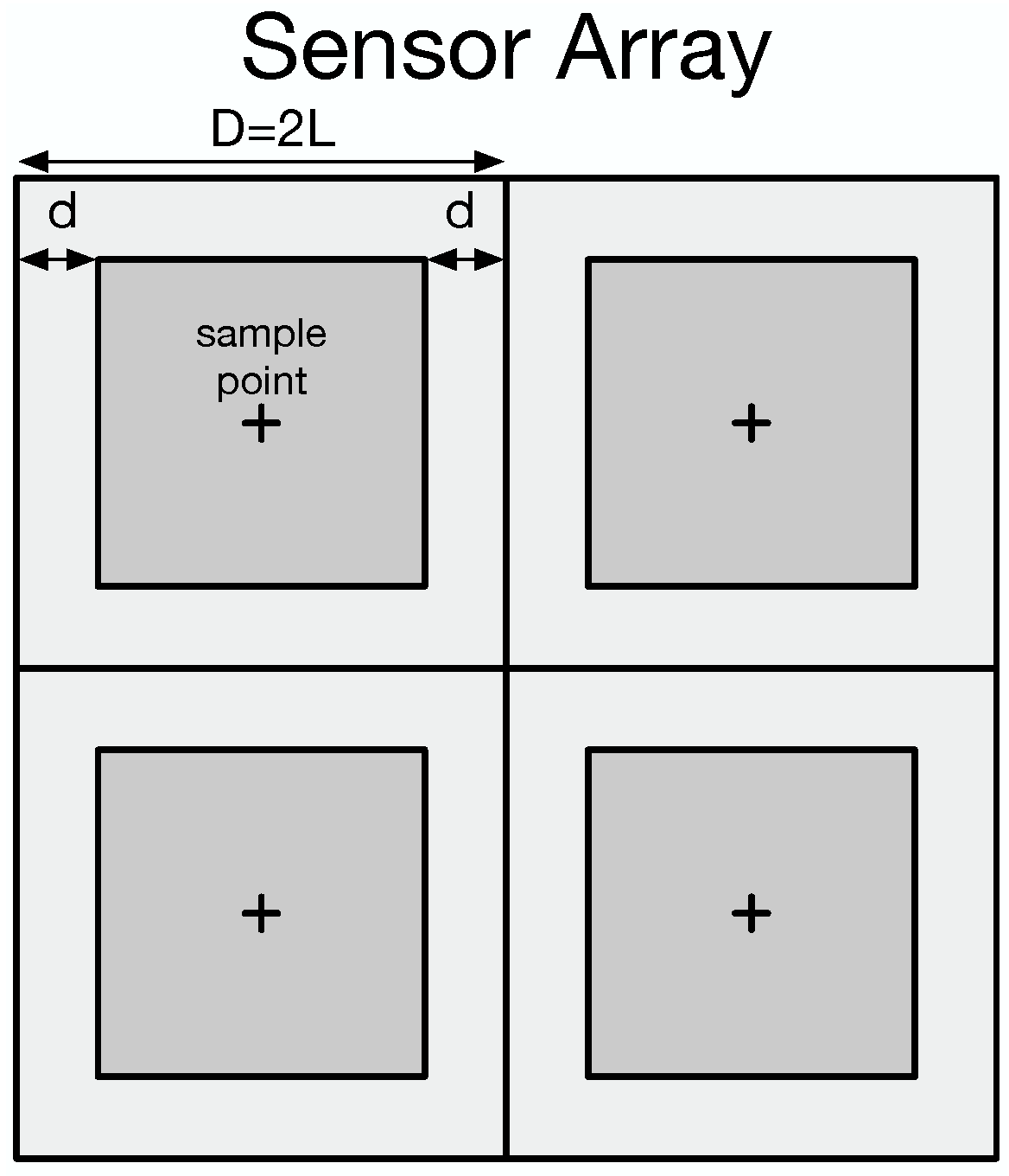
Figure 1. Geometric model for the sensor unit array. The grey area is the photon-sensitive area of the pixel. The cross points mark the centers of the pixels.
Universe 08 00593 g001
Figure 2. An brief illustration for the sampling effect. Consider a one-dimensional photon density distribution along the x-axis whose profile is noted as p ( x ) in (a). Suppose we sample the profile with an integral sampling array marked with the blue blocks in (b). The n t h sample X n differs from the n t h impulse sample X n by a slight deviation since X n is the red area below the profile (shown in (c)) while X n stands for the exact value of p ( x ) at the n t h sampling point (shown in (d)). X n and X n are usually unequal for an arbitrary photon density distribution.
Universe 08 00593 g002
Figure 3. Simulations for two-point sources collected by an imaging system with a Gaussian PSF shown in the pixel coordinate. The point sources are at ( 21 , 21 ) and ( 26 , 26 ) in pixel coordinate on the object plane. (a) is the impulse sample signal. (b) is the integral sample signal. (c) shows the recovered impulse signal from (b). (d) is the error image of (a,b). (e) is the error image of (a,d). (f) is the R matrix for this system.
Universe 08 00593 g003
Figure 4. Basic setup for the simulation. (a) is the PSF of the system. (b) is the response to uniform illumination by the asymmetric QE array, which represents the intra-pixel sensitivity distribution for the simulated asymmetric integral sampler array.
Universe 08 00593 g004
Figure 5. Simulations on the sampling process with (a) uniform integral sampler and (b) asymmetric integral sampler. (c) is the direct illumination on the asymmetric integral sampler.
Universe 08 00593 g005
Figure 6. A comparison among the uniform QE image, asymmetric QE image, and recovered QE image. (a) Recovered uniform QE Image. (b) Error between uniform and Asymmetric QE Images. (c) Error between Recovered and uniform QE Images.
Universe 08 00593 g006
Figure 7. Statistical results on position accuracy by random source positions with randomly distributed photons.
Universe 08 00593 g007
Figure 8. Error analysis about the PSF size and the sampling rate. The maximum relative error decreases rapidly to 10 15 as the PSF’s size increases.
Universe 08 00593 g008
Table 1. Influence of the asymmetric integral sampler on the position accuracy.
BarycenterX (Pixel)Y (Pixel)Relative Error
Ideal6.50006.5000
Uniform Integral Sampler6.50506.5050 7.69 × 10 4
Asymmetric Integral Sampler6.52116.5211 3.24 × 10 3
Table 2. Barycenter of the Image by the Recovered Uniform Integral Sampler.
BarycenterX (Pixel)Y (Pixel)Relative Error
Ideal Centroid6.50006.5000
Recovered Uniform Integral Sampler6.50516.5051 7.85 × 10 4
Table 3. Results of mean position measurement by uniform, asymmetric, and fixed integral samplers.
Position (Pixel)Xstd (X)Ystd (Y)
Ideal position29.4740.29029.5140.281
Uniform integral sampler29.4750.28829.5130.281
Asymmetric integral sampler29.4910.28929.5290.281
Fixed integral sampler29.4750.28929.5130.281
Table 4. Errors of mean position measurement by uniform, asymmetric, and fixed integral samplers.
Position (Pixel)Xstd (X)Ystd (Y)
Uniform error0.0010.006−0.0010.007
Asymmetric error0.0170.0060.0150.007
Fixed error0.0010.006−0.0010.007
Publisher’s Note: MDPI stays neutral with regard to jurisdictional claims in published maps and institutional affiliations.