The Primordial Particle Accelerator of the Cosmos

Abstract

In a previous paper we have shown that superluminal particles are allowed by the general relativistic theory of gravity provided that the metric is locally Euclidean. Here we calculate the probability density function of a canonical ensemble of superluminal particles as function of temperature. This is done for both space-times invariant under the Lorentz symmetry group, and for space times invariant under an Euclidean symmetry group. Although only the Lorentzian metric is stable for normal matter density, an Euclidian metric can be created under special gravitational circumstances and persist in a limited region of space-time consisting of the very early universe, which is characterized by extremely high densities and temperatures. Superluminal particles also allow attaining thermodynamic equilibrium at a shorter duration and suggest a rapid expansion of the matter density.

1. Introduction

A basic and well accepted fact is that space-time in the solar system can be approximately described by a Lorentz (Minkowski) metric ${\eta }_{\mu \nu }=\mathrm{diag}(1,-1,-1,-1)$ (Greek indices belong to the set $[0,1,2,3]$) and therefore physical theories are invariant under the Lorentz symmetry group.

Ref. [1] informs us that in the general theory of relativity (GR), the metric is locally ${\eta }_{\mu \nu }=\mathrm{diag}(1,-1,-1,-1)$, but not globally due to curvature. This is dictated by the principle of equivalence. Other requirements of GR including diffeomorphism invariance, and the Newtonian limit for weak gravity and slowly changing density profiles lead to the equations of Einstein:

$$G_{\mu \nu }=-\frac{8\pi G}{c^4}{T}_{\mu \nu }$$

(1)

here $G_{\mu \nu }$ stands for the Einstein tensor, $T_{\mu \nu }$ symbolizes the stress-energy tensor, G is the Newtonian universal gravitational constant and c is the speed of light in vacuum.

Does one need to postulate that space-time is locally Lorentz based on an empirical (unexplained) facts? The answer is no. This property can be derived from the field equations based on the stability of the Minkowskian solution [2]. Other unstable flat solutions of GR, which are of a non Minkowskian type, such as an Euclidian metric ${\eta }_{\mu \nu }=\pm \mathrm{diag}(1,1,1,1)$ can exist in a limited region of space-time, in which the physical equations will have an Euclidean symmetry group. In an Euclidian metric there are no speed limitations and thus the alleged particle can travel faster than the speed of light [3].

Eddington ([4], p. 25) has already studied the possibility that the universe contains different domains that are locally Lorentzian and others that have some other local metric such as ${\eta }_{\mu \nu }=\mathrm{diag}(-1,-1,-1,-1)$ or ${\eta }_{\mu \nu }=\mathrm{diag}(1,1,-1,-1)$. The stability of those domains was not discussed by Eddington.

One can find in the literature other explanations to the signature of the space-time metric [5,6,7,8], however, all other metric justifications rely on theoretical structures and assumptions that are external to GR and thus should be abandoned according to the Occam razor principle. Previous works [2,9,10,11] have shown that GR equations and linear stability analysis of the Lorentzian metric suffice to obtain a unique choice of the Lorentzian metric being the only one that is stable in an empty or almost empty space-time. Other allowed metrics are unstable and can thus exist in only a limited region of empty space-time. In the case of high density (such as the very early universe or near a black hole singularity) the situation is less certain [12]. The existence of the intuitive partition of a 4-dimensional space into space and time is conjectured to be a feature of an (almost) empty space-time. Such a partition is not a property of a general solutions of Einstein’s equations, such as the one discovered by Gödel [13]. However, this problem is not a characteristic of exotic space-times, but rather a property of standard cosmological models. We mention that the choice of coordinates in the Fisher approach to physics can also be justified using the above stability analysis [14]. Although the stability analysis of previous work is linear, we notice also the nonlinear stability analysis of the Lorentzian metric in Ref. [15]. We also point out that the nonlinear instability of a constant metric of different signatures remains an open question at this time.

Cosmological theory encounters many difficulties related to the horizon, flatness, entropy, and monopole problems [16]. A solution to these problems was introduced by Alan Guth using his famous cosmological inflation [17]. Entropy difficulties that remained in the original inflation model has led to a new cosmological inflation put forward by Linde [18], which solves the entropy problem at a price of fine tuned parameters. The same criticism is also relevant to chaotic inflation, also conjectured by Linde [19]. On 17 March 2014, astrophysicists of the BICEP2 group reported the detection of inflationary gravitational waves in the B-mode power spectrum, providing experimental evidence for the theory of inflation [20]. However, on 19 June 2014, the collaboration lowered confidence in confirming the findings.

There is a basic deficiency relevant to all inflation models, which require one or more ad hoc scalar fields. Those conjectured physical fields have no function, implication, or purpose in nature except for their use in the inflation model, which is in gross violation of the Occam razor principle. Occam’s razor principle demand that a minimum number of assumptions will explain a maximum number of phenomena (and not the other way around). Postulating a field to explain every phenomena does not serve the purpose of theoretical physics. As Einstein stated: “Everything should be made as simple as possible, but not simpler”.

This idea of an Euclidean metric in the early universe has attracted the attention of a long and distinguished list of authors including Sakharov [21,22], Hawking [23], and Ellis [24]. Sakharov’s work on the changes in the metrics signature was authored during an era in which quantum cosmology was a vibrant topic of research. It was influenced by the papers of Vilenkin [25], Hartle and Hawking [23], and others. Sakharov conjectured that the early beginning of the Universe is a result of a quantum transition from a spacetime with an Euclidean signature $(+1,+1,+1,+1)$ to a Lorentzian signature $(+1,-1,-1,-1)$. However, Sakharov has not given a detailed mathematical theory of this transition. As mentioned in Ref. [26], the idea became popular later. It was actively studied in 1990s (see, e.g., Ref. [27] and references mentioned therein). Different approaches exist to the change of metric; some are classical [28], while others are quantum [29,30]. Here we will not concern ourselves with the mechanism of metric change (however, the interested reader can refer to Ref. [3] in Section 2), but rather with the dynamics and statistical physics of the particles within a portion of space-time in which a metric with a specific signature prevails.

The plan of this paper is as follows: First we make a comment about the definition of time in an Euclidean space, after which we describe a particle trajectory in a general flat space. Then we analyze particle trajectories in Lorentz space-time for the standard subluminal and superluminal cases. The next section will discuss Euclidean metric dynamics. The final section is devoted to statistical analysis of free particles of the three different types (Euclidian, subluminal Lorentzian, and superluminal Lorentzian), in which we shall attempt to describe an equilibrium probability density function of a canonical ensemble of free particles. The possible physical implications of the current theory are then described. Finally, we make some concluding remarks.

2. The Definition of the Temporal Coordinate

Obviously for the Minkowski metric $(+1,-1,-1,-1)$, the underlying symmetry is Lorentz symmetry, and the plus sign (different from the three minus signs) singles out the time coordinate. A basic problem for Euclidean metric $(-1,-1,-1,-1)$ is how to define time. If the underlying symmetry is $SO\left(4\right)$, then all coordinates have the same meaning, so the first thing we need to do is to define time.

Notice, however, that if the universe was initially with a metric of signature (−1, −1, −1, −1) this type of solution would become unstable as the universe expands and the density decreases [2,9,11,12], eventually evolving into a solution with a Minkowski signature $(+1,-1,-1,-1)$. This involves a spontaneous symmetry breaking in an arbitrary direction, which will become the “time” coordinate. This resembles the situation of a pencil well balanced on its tip on a table. The pencil will eventually fall into some direction, but one cannot tell in advance into which direction it will fall, after falling the initial cylindrical symmetry is obviously broken, and the direction of falling can be assumed to become the axis $\theta =0$ for the azimuthal angel $\theta$.

Thus, in hindsight, we can distinguish one specific direction as a temporal direction, which we designate as the $x_0$ axis. This is the axis along which the symmetry has been broken. Thus, we can also designate the same direction that initially cannot be distinguished from any other direction as a temporal only because we know that after the universe reaches a certain expansion this will be recognized as different from the other directions.

3. Trajectories through Variational Analysis

We consider a particle traveling in spacetime of a constant metric with an unspecified signature. The action $\mathcal{A}$ of such a particle is:

$$\mathcal{A}=-mc\int d\tau -e\int A^{\alpha }d{x}_{\alpha }$$

(2)

In the above $\tau$ is the trajectory interval:

$$d{\tau }^2=\left|{\eta }^{\alpha \beta }d{x}_{\alpha }d{x}_{\beta }\right|=\left|d{x}_{\alpha }d{x}^{\alpha }\right|$$

(3)

$x_{\alpha }$ are the particle coordinates (the metric raises and lowers indices according to the prevailing custom), m is the particle mass, e is the charge, and $A^{\alpha }$ is the four vector potential that depends on the particle coordinates. $A^{\alpha }$ transforms as a four-dimensional vector. Variational analysis results in the following equations of motion:

$$m\frac{d{u}^{\alpha }}{d\tau }=-\frac{e}{c}{u}^{\beta }({\partial }_{\beta }{A}^{\alpha }-{\partial }^{\alpha }{A}_{\beta }),u^{\alpha }\equiv \frac{d{x}^{\alpha }}{d\tau }$$

(4)

in which the metric ${\eta }_{\alpha \beta }$ can be of any flat type: Lorentzian, Euclidean, etc.

3.1. Lorentz Space-Time

Given a space-time with a Lorentz metric ${\eta }_{\mu \nu }=\mathrm{diag}(1,-1,-1,-1)$ the partition into spatial and temporal coordinates is trivial. The spatial coordinates are $\overrightarrow{x}=(x_1,x_2,x_3)$ and the temporal coordinate is $x_0$. As we measure time in the units of seconds, which differ from the space units of meters, we introduce $x_0=ct$, in which c connects the different units. The velocity is defined as: $\overrightarrow{v}\equiv \frac{d\overrightarrow{x}}{dt},v=|\overrightarrow{v}|$. In a similar way we dissect $A_{\alpha }$ into temporal and spatial pieces:

$$A_{\alpha }=(A_0,A_1,A_2,A_3)\equiv (A_0,\overrightarrow{A})\equiv (\frac{\varphi }{c},\overrightarrow{A})$$

(5)

the factor $\frac{1}{c}$ in the last term allows us to obtain the equations in MKS units, and it is not needed in other types of unit systems. Through Equation (5), we can define a magnetic field:

$$\overrightarrow{B}=\overrightarrow{\nabla }\times \overrightarrow{A}$$

(6)

($\overrightarrow{\nabla }$ has the standard meaning) and the electric field:

$$\overrightarrow{E}=-\frac{\partial \overrightarrow{A}}{\partial t}-\overrightarrow{\nabla }\varphi$$

(7)

For the subluminal case $v<c$ we may write $d{\tau }^2$ as:

$$d{\tau }^2=c^{2}d{t}^2(1-\frac{v^2}{c^2}),d\tau =cdt\sqrt{1-\frac{v^2}{c^2}}$$

(8)

Using the above equations, the spatial piece of Equation (4) is deduced:

$$\frac{d}{dt}\left(m\frac{\overrightarrow{v}}{\sqrt{1-\frac{v^2}{c^2}}}\right)=e\left(\overrightarrow{E}+\overrightarrow{v}\times \overrightarrow{B}\right)$$

(9)

The above demonstrated that a particle subluminal in a Lorentz space must remain subluminal. This follows because as the particle is accelerated to the velocity of light, its “effective mass” $m_{eff}\equiv \frac{m}{\sqrt{1-\frac{v^2}{c^2}}}$ becomes unbounded. On the other hand, for superluminal particles ($v>c$ initially), we may write $d{\tau }^2$ as:

$$d{\tau }^2=c^{2}d{t}^2(\frac{v^2}{c^2}-1),d\tau =cdt\sqrt{\frac{v^2}{c^2}-1}$$

(10)

Using the above equations we derive the spatial piece of Equation (4) in the form:

$$\frac{d}{dt}\left(m\frac{\overrightarrow{v}}{\sqrt{\frac{v^2}{c^2}-1}}\right)=e\left(\overrightarrow{E}+\overrightarrow{v}\times \overrightarrow{B}\right)$$

(11)

Here the difficulty would be to reduce the velocity, as the superluminal “effective mass” $m_{eff}\equiv \frac{m}{\sqrt{\frac{v^2}{c^2}-1}}$ becomes unbounded. As infinite forces are not available in any physical scenario, the velocity of the above particle must remain superluminal. Thus, in a Lorentz space time it is impossible to pass the velocity c from above.

The case of a luminal particle with $v=c$ has $d\tau =0$, which makes this parameter unsuitable to describe the trajectory for those type of particles (photons).

3.2. Euclidean Space-Time

An Euclidean space-time possesses a metric of the type ${\eta }_{\mu \nu }=\mathrm{diag}(+1,+1,+1,+1)$. Thus, space-time points are labeled (arbitrarily) by spatial and temporal coordinates in a similar way to the Lorentz case and are measured in the standard units. $A_{\alpha }$ is partitioned into temporal and spatial pieces as defined in Equation (5). We may still define a magnetic field as in Equation (6) but the electric field must be defined differently:

$$\overrightarrow{E}=-\frac{\partial \overrightarrow{A}}{\partial t}+\overrightarrow{\nabla }\varphi$$

(12)

in order to preserve Faraday’s law. For both subluminal or superluminal particles, we may write $d{\tau }^2$ as:

$$d{\tau }^2=c^{2}d{t}^2(1+\frac{v^2}{c^2}),d\tau =cdt\sqrt{1+\frac{v^2}{c^2}}$$

(13)

Using the above equations, the spatial piece of Equation (4) becomes:

$$\frac{d}{dt}\left(m\frac{\overrightarrow{v}}{\sqrt{1+\frac{v^2}{c^2}}}\right)=e\left(\overrightarrow{E}-\overrightarrow{v}\times \overrightarrow{B}\right)$$

(14)

The above shows that particles in an Euclidean space are indifferent to passing the velocity c from below or above.

4. Statistical Physics

The definition of a probability density function is intimately connected to the notion of phase space. This in turn arises naturally when time is the independent variational variable. The path to the Hamiltonian formalism goes through defining a Lagrangian at the action per unit time and through the Lagrangian one can define the canonical momenta and finally the Hamiltonian. We shall follow this route.

4.1. Lagrangian and Canonical Momenta

Let us write the action given in Equation (2) as:

$$\mathcal{A}=-mc\int d\tau -e\int A^{\alpha }d{x}_{\alpha }=-\int dt\left[mc\frac{d\tau }{dt}+e{A}^{\alpha }\frac{d{x}_{\alpha }}{dt}\right]$$

(15)

Introducing the notation:

$$v_{\alpha }\equiv \frac{d{x}_{\alpha }}{dt}=(c,\overrightarrow{v})$$

(16)

and using the definition of Equation (3) it follows that:

$$\frac{d\tau }{dt}=\sqrt{\left|\frac{d{x}_{\alpha }}{dt}\frac{d{x}^{\alpha }}{dt}\right|}=\sqrt{\left|v_{\alpha }{v}^{\alpha }\right|}=\sqrt{\left|c^2+v_i{v}^i\right|}$$

(17)

in which the Latin indices are $i\in \{1,2,3\}$. The upper index $v^i$ has the following meaning:

$$v^i=\left\{\begin{array}{cc}+v_i& \mathrm{Euclidean}\mathrm{metric}\\ -v_i& \mathrm{Lorentz}\mathrm{metric}\end{array}\right.$$

(18)

Thus:

$$\begin{array}{ccc}\hfill \frac{d\tau }{dt}& =& \left\{\begin{array}{cc}\sqrt{\left|c^2+{\overrightarrow{v}}^2\right|}& \mathrm{Euclidean}\mathrm{metric}\\ \sqrt{\left|c^2-{\overrightarrow{v}}^2\right|}& \mathrm{Lorentz}\mathrm{metric}\end{array}\right.\hfill \\ & =& \left\{\begin{array}{cc}\sqrt{c^2+v^2}& \mathrm{Euclidean}\mathrm{metric}\\ \sqrt{c^2-v^2}& \mathrm{Lorentz}\mathrm{metric}\mathrm{subluminal}\mathrm{case}v<c\\ \sqrt{v^2-c^2}& \mathrm{Lorentz}\mathrm{metric}\mathrm{superluminal}\mathrm{case}v>c\end{array},\right.\hfill \end{array}$$

(19)

It follows from Equation (15) that one can define a Lagrangian:

$$\begin{array}{ccc}\hfill \mathcal{A}=\int dtL,L& \equiv & -\left[mc\frac{d\tau }{dt}+e{A}^{\alpha }\frac{d{x}_{\alpha }}{dt}\right]=-\left[mc\sqrt{\left|v_{\alpha }{v}^{\alpha }\right|}+e{A}^{\alpha }{v}_{\alpha }\right]\hfill \\ & =& -\left[mc\sqrt{\left|c^2+v_i{v}^i\right|}+ec{A}^0+e{A}^i{v}_i\right].\hfill \end{array}$$

(20)

This leads to a canonical momentum of the form:

$$p^i\equiv \frac{\partial L}{\partial v_i}=-mc\frac{\pm v^i}{\sqrt{\left|c^2+v_i{v}^i\right|}}-e{A}^i$$

(21)

the sign is decided according to whether the absolute value changes or does not change the sign of $c^2+v_i{v}^i$. It does not change the sign of course in the standard subluminal Lorentzian case but also the Euclidean case. On the other the superluminal Lorentzian case involves a sign change. Hence:

$$p^i=\left\{\begin{array}{cc}-mc\frac{v^i}{\sqrt{\left|c^2+v_i{v}^i\right|}}-e{A}^i& \mathrm{Lorentzian}\mathrm{subluminal}\mathrm{or}\mathrm{Euclidean}\\ +mc\frac{v^i}{\sqrt{\left|c^2+v_i{v}^i\right|}}-e{A}^i& \mathrm{Lorentzian}\mathrm{superluminal}\end{array}\right.$$

(22)

Introducing the standard notation:

$${\beta }_i\equiv \frac{v_i}{c},{\beta }^i\equiv \frac{v^i}{c},\beta \equiv \frac{v}{c},\gamma \equiv \frac{1}{\sqrt{\left|1+\frac{v_i{v}^i}{c^2}\right|}}=\frac{1}{\sqrt{\left|1+{\beta }_i{\beta }^i\right|}}$$

(23)

in which:

$$\gamma =\left\{\begin{array}{cc}\frac{1}{\sqrt{1+\frac{v^2}{c^2}}}& \mathrm{Euclidean}\mathrm{metric}\\ \frac{1}{\sqrt{1-\frac{v^2}{c^2}}}& \mathrm{Lorentz}\mathrm{metric}\mathrm{subluminal}\mathrm{case}v<c\\ \frac{1}{\sqrt{\frac{v^2}{c^2}-1}}& \mathrm{Lorentz}\mathrm{metric}\mathrm{superluminal}\mathrm{case}v>c\end{array}\right..$$

(24)

We may write:

$$p^i=\left\{\begin{array}{cc}-\gamma m{v}^i-e{A}^i& \mathrm{Lorentzian}\mathrm{subluminal}\mathrm{or}\mathrm{Euclidean}\\ +\gamma m{v}^i-e{A}^i& \mathrm{Lorentzian}\mathrm{superluminal}\end{array}\right.$$

(25)

We can define a “free” momentum as:

$$p_f^i=p^i+e{A}^i=\left\{\begin{array}{cc}-\gamma m{v}^i& \mathrm{Lorentzian}\mathrm{subluminal}\mathrm{or}\mathrm{Euclidean}\\ +\gamma m{v}^i& \mathrm{Lorentzian}\mathrm{superluminal}\end{array}\right.$$

(26)

this is a misnomer, as the case $A^i=0$ includes the free particle case but also applies to the case in which the particle moves under the influence of a scalar electric potential. By defining a canonical momentum vector, we have:

$$\overrightarrow{p}\equiv (p^1,p^2,p^3)=\left\{\begin{array}{cc}\gamma m\overrightarrow{v}+e\overrightarrow{A}& \mathrm{Lorentzian}\mathrm{subluminal}\\ -\gamma m\overrightarrow{v}-e\overrightarrow{A}& \mathrm{Euclidean}\\ -\gamma m\overrightarrow{v}+e\overrightarrow{A}& \mathrm{Lorentzian}\mathrm{superluminal}\end{array}\right.$$

(27)

in which we have used Equation (18) and also:

$$A^i=\left\{\begin{array}{cc}+A_i& \mathrm{Euclidean}\mathrm{metric}\\ -A_i& \mathrm{Lorentz}\mathrm{metric}.\end{array}\right.$$

(28)

Similarly:

$${\overrightarrow{p}}_f\equiv (p_f^1,p_f^2,p_f^3)=\left\{\begin{array}{cc}\gamma m\overrightarrow{v}& \mathrm{Lorentzian}\mathrm{subluminal}\\ -\gamma m\overrightarrow{v}& \mathrm{Euclidean}\\ -\gamma m\overrightarrow{v}& \mathrm{Lorentzian}\mathrm{superluminal}.\end{array}\right.$$

(29)

Interestingly the “free” momentum has the same direction as the velocity only in the (standard) Lorentzian subluminal case; in all other cases the momentum direction is the opposite. The Lorentzian subluminal case reduces to the classical result for low velocities:

$$v\ll c\Rightarrow \gamma \simeq 1\Rightarrow \overrightarrow{p}\simeq m\overrightarrow{v}+e\overrightarrow{A}$$

(30)

In all cases the magnitude of the “free” momentum is:

$$p_f=\left|{\overrightarrow{p}}_f\right|=\gamma mv.$$

(31)

Thus, a subluminal Lorentzian “free” particle will have zero momentum for $v=0$ and infinite momentum for $v=c$, in which the momentum is an increasing function of v (see Figure 1). Hence, the phase space is non compact. In the Euclidean case, the small velocity momentum is similar to the Lorentzian case, however, the momentum space in this case is limited inside a “momentum sphere”; hence, it is compact. Thus a subluminal Lorentzian “free” particle will have zero momentum for $v=0$ and a momentum of $p_{fE}=mc$ for $v=\infty$. The momentum is an increasing function of velocity, which is bounded (see Figure 2 and Figure 3). Finally for a superluminal Lorentzian particle we have $p_{fLsup}=\infty$ for the case $v=c$ and $p_{fLsup}=mc$ for the case $v=\infty$. The momentum is a decreasing function of velocity (see Figure 4), which differs considerably from our habits and physical intuition. The momentum space is not compact, however, it has spherical hole in its middle of radius $mc$. One could say that the set union of the momentum space in the Euclidean case and the momentum space in the superluminal Lorentzian case is equal to the momentum space of the subluminal Lorentzian case. This situation is depicted in Figure 5. In terms of the $\gamma$ notation, we can write the Lagrangian as:

$$L=-\left[\frac{m{c}^2}{\gamma }+ec{A}^0+e{A}^i{v}_i\right].$$

(32)

For small velocities in a Lorentzian space time we have:

$$\gamma \simeq 1+\frac{1}{2}\frac{v^2}{c^2},{\gamma }^{-1}\simeq 1-\frac{1}{2}\frac{v^2}{c^2}.$$

(33)

Hence, the classical Lagrangian would be:

$$L_c=\frac{1}{2}m{v}^2-(m{c}^2+e\varphi -e\overrightarrow{A}·\overrightarrow{v})=\frac{1}{2}m{v}^2+e\overrightarrow{A}·\overrightarrow{v}-e\varphi -m{c}^2.$$

(34)

Finally, we will be interested in the dependence of v on $p_f$. We first notice that:

$$m\gamma =\frac{p_f}{v}\Rightarrow m^2{v}^2=p_f^2{\gamma }^{-2}=p_f^2\left|1+\frac{v_i{v}^i}{c^2}\right|.$$

(35)

Thus, we obtain:

$$v=\left\{\begin{array}{cc}\frac{p_f}{\sqrt{m^2+\frac{p_f^2}{c^2}}}& \mathrm{Lorentzian}\mathrm{subluminal}\\ \frac{p_f}{\sqrt{m^2-\frac{p_f^2}{c^2}}}& \mathrm{Euclidean}\\ \frac{p_f}{\sqrt{\frac{p_f^2}{c^2}-m^2}}& \mathrm{Lorentzian}\mathrm{superluminal}\end{array}\right.$$

(36)

4.2. Hamiltonian and Energy

Once we have the canonical momenta and Lagrangian, it is straightforward to calculate the Hamiltonian:

$$\begin{array}{ccc}\hfill H& =& \overrightarrow{v}·\overrightarrow{p}-L=p^i{v}_i-L=p^i{v}_i+\frac{m{c}^2}{\gamma }+ec{A}^0+e{A}^i{v}_i\hfill \\ & =& (\mp \gamma m{v}^i-e{A}^i)v_i+\frac{m{c}^2}{\gamma }+ec{A}^0+e{A}^i{v}_i=\mp \gamma m{v}^i{v}_i+\frac{m{c}^2}{\gamma }+ec{A}^0.\hfill \end{array}$$

(37)

in the above, the minus sign is for the Euclidean and subluminal Lorentzian cases while the plus sign is for the superluminal Lorentzian case. This can be simplified as follows:

$$\begin{array}{ccc}\hfill H& =& \gamma m(\mp v^i{v}_i+\frac{c^2}{{\gamma }^2})+e\varphi =\gamma m\left(\mp v^i{v}_i+c^2\left|1+{\beta }_i{\beta }^i\right|\right)+e\varphi \hfill \\ & =& \gamma m\left(\mp v^i{v}_i+\left|c^2+v_i{v}^i\right|\right)+e\varphi =\pm \gamma m{c}^2+e\varphi .\hfill \end{array}$$

(38)

The plus sign in the last terms belongs to the Euclidean and subluminal Lorentzian cases, while the minus sign is for the superluminal Lorentzian case. Explicitly:

$$H=\left\{\begin{array}{cc}\gamma m{c}^2+e\varphi & \mathrm{Euclidean}\mathrm{and}\mathrm{subluminal}\mathrm{Lorentzian}\\ -\gamma m{c}^2+e\varphi & \mathrm{superluminal}\mathrm{Lorentzian}\end{array}\right.$$

(39)

The energy of the particle is $En=H$ and will remain constant as long as $\varphi$ does not explicitly depend on time. The structure of the Hamiltonian is:

$$H=E_k+e\varphi$$

(40)

in which:

$$E_k\equiv \left\{\begin{array}{cc}\frac{m{c}^2}{\sqrt{1+\frac{v^2}{c^2}}}& \mathrm{Euclidean}\mathrm{metric}\\ \frac{m{c}^2}{\sqrt{1-\frac{v^2}{c^2}}}& \mathrm{Lorentz}\mathrm{metric}\mathrm{subluminal}\mathrm{case}v<c\\ -\frac{m{c}^2}{\sqrt{\frac{v^2}{c^2}-1}}& \mathrm{Lorentz}\mathrm{metric}\mathrm{superluminal}\mathrm{case}v>c\end{array}\right..$$

(41)

The kinetic energy has the following attributes. For the Lorentz subluminal case (which is the standard case), the minimal value for the kinetic energy is the remaining energy $E_{kLsubmin}=m{c}^2$ obtained for $v=0$. However, it can reach an infinite value for velocities approaching the speed of light in vacuum c:

$$E_{kLsubmax}=\underset{v\to c}{lim}{E}_{kLsub}=+\infty .$$

(42)

It is always positive for all values of v. In the classical case in which $v\ll c$, we can partition the energy into a “classical kinetic energy” and a rest energy:

$$E_{kLsub}\simeq m{c}^2+E_{kLsubc},E_{kLsubc}\equiv \frac{1}{2}m{v}^2,v\ll c.$$

(43)

The expression $E_{kLsub}$ is depicted in Figure 6. In the Euclidean case, the kinetic energy is always positive, as it has a maximal value for a particle in rest: $E_{kEmax}=m{c}^2$ and a minimal value of zero for a particle traveling at an infinite speed. We recall that there are no speed limitations in an Euclidean space-time.

$$E_{kEmin}=\underset{v\to +\infty }{lim}{E}_{kE}=0.$$

(44)

Curiously, one can define a “classical kinetic energy” also in the Euclidean case, but it will be negative:

$$E_{kE}\simeq m{c}^2+E_{kEc},E_{kEc}\equiv -\frac{1}{2}m{v}^2,v\ll c.$$

(45)

The expression $E_{kE}$ is depicted in Figure 7 for subluminal velocities and in Figure 8 for superluminal velocities. Finally we consider the superluminal Lorentzian kinetic energy, which differs from the previous cases in the attribute that it is always non positive. Its maximal value of zero is attained for infinite velocities and it can reach minus infinity when the velocity of the particle is reduced down to the speed of light c, a limit it cannot reach. Thus:

$$E_{kLsupmax}=\underset{v\to +\infty }{lim}{E}_{kLsup}=0,E_{kLsupmin}=\underset{v\to c}{lim}{E}_{kLsup}=-\infty .$$

(46)

of course there is no sense of discussing the classical limit in this case, as by definition superluminality requires $v>c$. The expression $E_{kLsup}$ is depicted in Figure 9. Let us suppose that the potentials are time independent and the energy is conserved; it then follows that the energy $En$ is conserved and for any two points ${\overrightarrow{x}}_1$ and ${\overrightarrow{x}}_2$ on the trajectory:

$$En=E_{k1}+e{\varphi }_1=E_{k2}+e{\varphi }_2\Rightarrow E_{k2}=E_{k1}+e({\varphi }_1-{\varphi }_2)$$

(47)

Thus, the kinetic energy can be increased or decreased using a potential difference, this is of course well known and is used for accelerating and decelerating charged particles in electrostatic accelerators like the tandem accelerator located in Ariel university [31]. For a subluminal particle, an increase in the kinetic energy means an increase in velocity; thus, by using a potential difference, a charged particle can be accelerated. Similarly, by using a potential difference with an opposite sign, the particle becomes slower as its kinetic energy is reduced. For Euclidean particles, the situation is opposite, as particles with higher kinetic energy are slower and particles with low kinetic energy are faster. Nevertheless, potential differences can be still used to achieve acceleration and deceleration. Superluminal Lorentzian particles are similar to the subluminal Lorentzian particles in the sense that the (negative) kinetic energy would be lower for slower particles and higher for faster particles. Another important difference between Euclidean and Lorentzian particles is the lack of velocity limits in the former. In fact, it is easy to see that by using a finite energy equal to its rest mass ($m{c}^2$), a particle can be accelerated from zero velocity to infinite velocity in an Euclidean space-time. This is of course impossible for a Lorentzian particle. In the sub luminal case we will need an infinite amount of energy to accelerate the particle to the speed of light, while for a superluminal particle an infinite amount of energy will be needed to reduce its speed to the speed of light. This entails an infinite potential difference and thus is physically impossible. We remark that even if the electromagnetic potentials are time dependent (as in the popular accelerator scheme of RF Linacs [32]) this limitation cannot be avoided because although the total energy of the particle can be increased in this scenario and is not necessarily constant, it cannot increase to infinite values (which should be supplied from an infinite reservoir). Thus, in a Lorentzian universe, subluminal and superluminal particles must be separated by their velocities forever. We will discuss the cosmological and other implications of those facts later in this paper.

To conclude this subsection, we would like to express the Hamiltonian as a function of the coordinates and the momenta. Using Equation (39) and Equations (35) and (36), this can be written as follows:

$$H=\left\{\begin{array}{cc}{c}^2\sqrt{m^2+\frac{p_f^2}{c^2}}+e\varphi & \mathrm{Lorentzian}\mathrm{subluminal}\\ c^2\sqrt{m^2-\frac{p_f^2}{c^2}}+e\varphi & \mathrm{Euclidean}\\ -c^2\sqrt{\frac{p_f^2}{c^2}-m^2}+e\varphi & \mathrm{Lorentzian}\mathrm{superluminal}\end{array}\right..$$

(48)

For Lorentzian classical particles Equation (30) holds, hence $p_f\simeq mv$ and thus:

$$H_c\simeq m{c}^2+\frac{p_f^2}{2m}+e\varphi$$

(49)

Using Equation (26), we arrive at:

$$H(\overrightarrow{x},\overrightarrow{p})=\left\{\begin{array}{cc}{c}^2\sqrt{m^2+\frac{{(\overrightarrow{p}-e\overrightarrow{A}\left(\overrightarrow{x}\right))}^2}{c^2}}+e\varphi \left(\overrightarrow{x}\right)& \mathrm{Lorentzian}\mathrm{subluminal}\\ c^2\sqrt{m^2-\frac{{(\overrightarrow{p}+e\overrightarrow{A}\left(\overrightarrow{x}\right))}^2}{c^2}}+e\varphi \left(\overrightarrow{x}\right)& \mathrm{Euclidean}\\ -c^2\sqrt{\frac{{(\overrightarrow{p}-e\overrightarrow{A}\left(\overrightarrow{x}\right))}^2}{c^2}-m^2}+e\varphi \left(\overrightarrow{x}\right)& \mathrm{Lorentzian}\mathrm{superluminal}\end{array}\right.$$

(50)

the first line in the above is Jackson’s [33] formula (12.17). In the classical case, we have:

$$H_c(\overrightarrow{x},\overrightarrow{p})\simeq m{c}^2+\frac{{(\overrightarrow{p}-e\overrightarrow{A}\left(\overrightarrow{x}\right))}^2}{2m}+e\varphi \left(\overrightarrow{x}\right)$$

(51)

4.3. Statistical Physics of “Classical” Particles

Once we have a phase space, we may discuss what form the probability density function for a particle to be in a specific part of this space should be. Elementary considerations show [34] that in thermal equilibrium, this function must depend on the constants of motion of the system, in particular its energy.

$$f_{system}=f_{system}\left(H\right)=f_{system}\left(E_{system}\right)$$

(52)

Further, if the system can be partitioned into two sub systems A and B of which the interaction is negligible (as in the case of free particles) it follows that:

$$f_{system}\left(E_{system}\right)=f_{system}(E_A+E_B)=f_A\left(E_A\right)f_B\left(E_B\right)$$

(53)

This leads after a few trivial steps to the result that:

$$f=\frac{e^{-{\beta }_{T}H}}{Z}$$

(54)

Z the normalization constant, also known as the partition function. ${\beta }_T=\frac{1}{k_{B}T}$, in which $k_B$ is the Boltzmann constant:

$$k_B\equiv 1.380649{10}^{-23}{\mathrm{m}}^2\mathrm{kg}{\mathrm{s}}^{-2}{\mathrm{K}}^{-1}$$

(55)

and T is the temperature measured in degrees Kelvin. In what follows we will consider only free particles; moreover, we will consider only a single free particle. In this case:

$$Z=\int e^{-{\beta }_{T}H}{d}^{3}p$$

(56)

In all the relevant cases H depends only the absolute value $p=|\overrightarrow{p}|$, hence the integral simplifies to:

$$Z=4\pi \int e^{-{\beta }_{T}H}{p}^{2}dp$$

(57)

We will start with the more familiar case of a subluminal Lorentzian particle and consider the more exotic cases later.

4.3.1. A Low Speed Lorentzian Particle

For a small velocity free Lorentzian particle, Equation (51) takes the form:

$$H_c=m{c}^2+\frac{p^2}{2m}$$

(58)

hence:

$$f(\overrightarrow{p})=\frac{e^{-{\beta }_{T}m{c}^2}{e}^{-{\beta }_T\frac{p^2}{2m}}}{Z}.$$

(59)

The partition function can be calculated to be:

$$Z=4\pi \int e^{-{\beta }_T{H}_c}{p}^{2}dp={\left(2\pi m{k}_{B}T\right)}^{\frac{3}{2}}{e}^{-{\beta }_{T}m{c}^2}$$

(60)

Thus, we obtain the well known Maxwell–Boltzmann probability density function:

$$f\left(\overrightarrow{p}\right)=\frac{e^{-\frac{p^2}{2m{k}_{B}T}}}{{\left(2\pi m{k}_{B}T\right)}^{\frac{3}{2}}}.$$

(61)

This is a typical Gaussian distribution with a null average and a variance that is linear in the temperature and a standard deviation, which is the square root of the same:

$$E\left[p^i\right]=0,E\left[{p^i}^2\right]=m{k}_{B}T,{\sigma }_{p^i}=\sqrt{m{k}_{B}T}.$$

(62)

Using Equation (43), we obtain the well-known result for the average of the classical kinetic energy:

$$E\left[E_{kLsubc}\right]=E\left[\frac{1}{2}m{v}^2\right]=E\left[\frac{p^2}{2m}\right]=\frac{3m{k}_{B}T}{2m}=\frac{3}{2}{k}_{B}T$$

(63)

Thus, the average of the total kinetic energy, which includes a rest energy term:

$$E\left[E_{kLsub}\right]\simeq m{c}^2+\frac{3}{2}{k}_{B}T.$$

(64)

In what follows, expressions will appear simpler using a normalized momenta and ${\beta }_T$ is defined as follows:

$${\overrightarrow{p}}^{\prime }\equiv \frac{\overrightarrow{p}}{mc},\lambda \equiv {\beta }_{T}m{c}^2=\frac{m{c}^2}{k_{B}T}.$$

(65)

Thus, low $\lambda$ means high temperature, and high $\lambda$ means low temperature. In terms of this, we may write the classical distribution as:

$$f({\overrightarrow{p}}^{\prime })={(\frac{\lambda }{2\pi })}^{\frac{3}{2}}{e}^{-\frac{\lambda p^{\prime 2}}{2}},Z^{\prime }={(\frac{2\pi }{\lambda })}^{\frac{3}{2}}{e}^{-\lambda }.$$

(66)

Thus:

$$\underset{\lambda \to 0}{lim}{Z}^{\prime }=\infty ,\underset{\lambda \to \infty }{lim}{Z}^{\prime }=0.$$

(67)

In terms of $\lambda$, the average energy becomes:

$${\overline{E}}_{kLsub}^{\prime }=\frac{E\left[E_{kLsub}\right]}{m{c}^2}\simeq 1+\frac{3}{2\lambda }$$

(68)

for high $\lambda$ (low velocities).

4.3.2. A Lorentzian Particle

Generally speaking, the Maxwell–Boltzmann probability density function does not describe the momentum distribution function for a Lorentzian particle unless the velocities are much smaller than the speed of light. Taking into account Equation (50) for a free particle, and Equation (54) we arrive at:

$$f\left({\overrightarrow{p}}^{\prime }\right)=\frac{e^{-{\beta }_{T}H}}{Z^{\prime }}=\frac{e^{-\lambda \sqrt{1+p^{\prime 2}}}}{Z^{\prime }}$$

(69)

in which:

$$Z^{\prime }\left(\lambda \right)=4\pi {\int }_0^{\infty }{e}^{-\lambda \sqrt{1+p^{\prime 2}}}{p}^{\prime 2}d{p}^{\prime }$$

(70)

The above expression cannot be evaluated analytically, but can be easily evaluated numerically (see Figure 10) in which we compare the results to the classical case. As can be clearly seen, the results converge for high $\lambda$ (low temperature) but differ considerably for small $\lambda$ (high temperature). For a Lorentzian subluminal particle we have:

$$\underset{\lambda \to 0}{lim}{Z}^{\prime }=\infty ,\underset{\lambda \to \infty }{lim}{Z}^{\prime }=0,$$

(71)

the above result is similar to the case of a classical particle. Having calculated the partition function we are now in a position to calculate the probability density function. We present a two-dimensional plot in Figure 11, and two cross-sections for low and high $\lambda$ in Figure 12 and Figure 13. It is clear that the Maxwell–Boltzmann approximation is only appropriate for low temperatures (high $\lambda$) but fails completely at high temperatures. Finally, we calculate the average energy:

$$\begin{array}{ccc}\hfill {\overline{E}}_{kLsub}^{\prime }\left(\lambda \right)& =& \frac{E\left[E_{kLsub}\right]}{m{c}^2}=E\left[\sqrt{1+p^{\prime 2}}\right]=4\pi {\int }_0^{\infty }\sqrt{1+p^{\prime 2}}f\left({\overrightarrow{p}}^{\prime }\right)p^{\prime 2}d{p}^{\prime }\hfill \\ & =& \frac{4\pi }{Z^{\prime }\left(\lambda \right)}{\int }_0^{\infty }\sqrt{1+p^{\prime 2}}{e}^{-\lambda \sqrt{1+p^{\prime 2}}}{p}^{\prime 2}d{p}^{\prime }=-\frac{1}{Z^{\prime }\left(\lambda \right)}\frac{d{Z}^{\prime }\left(\lambda \right)}{d\lambda }=-\frac{dln{Z}^{\prime }\left(\lambda \right)}{d\lambda }\hfill \end{array}$$

(72)

this expression can be evaluated numerically and is depicted in Figure 14 for high $\lambda$ and Figure 15 for low $\lambda$. Again we notice that the classical approximation is only valid for high $\lambda$ (low temperature). In any case (exact or approximated) the average energy is a decreasing function of $\lambda$ or an increasing function of temperature, as might be expected. However, for Euclidean particles the results are less intuitive, as will be shown below.

4.3.3. An Euclidean Particle

As we saw in previous sections, Euclidean particles share with the Lorentzian particle the energy positivity property. However, they differ in the structure of their phase space considerably. Thus, taking into account Equation (50) for a free particle, and Equation (54) we arrive at:

$$f\left({\overrightarrow{p}}^{\prime }\right)=\frac{e^{-{\beta }_{T}H}}{Z^{\prime }}=\frac{e^{-\lambda \sqrt{1-p^{\prime 2}}}}{Z^{\prime }}$$

(73)

in which:

$$Z^{\prime }\left(\lambda \right)=4\pi {\int }_0^1{e}^{-\lambda \sqrt{1-p^{\prime 2}}}{p}^{\prime 2}d{p}^{\prime }$$

(74)

we recall that a free Euclidean particle phase space is compact and that $0\le p^{\prime }\le 1$. The above expression cannot be evaluated analytically, but can be easily evaluated numerically (see Figure 16). As can be clearly seen the partition function is a decreasing function of $\lambda$ or an increasing function of temperature. For an Euclidean particle we have:

$$\underset{\lambda \to 0}{lim}{Z}^{\prime }=\frac{4\pi }{3},\underset{\lambda \to \infty }{lim}{Z}^{\prime }=0,$$

(75)

Having calculated the partition function we are now in a position to calculate the probability density function. We present a two-dimensional plot in Figure 17, and a cross-section in Figure 18. It is remarkable that it is more probable to find an Euclidean particle with high momentum than with low momentum. This is in sharp contradiction to the situation for Lorentzian subluminal particles that prefer to stay in lower momenta. Of course, in both cases high momenta means high velocity. However, this fact correlates well with the energy being a decreasing function of velocity in the Euclidean case. Figure 18 shows that for an Euclidean space-time, the thermal equilibrium prefers superluminal velocities over subluminal velocities, as the former are much more probable. We remind the reader that Euclidean space time in the early universe was considered by many distinguished scientists such as Sakharov, Hawking, and Ellis.

Finally, we calculate the average energy:

$$\begin{array}{ccc}\hfill {\overline{E}}_{kE}^{\prime }\left(\lambda \right)& =& \frac{E\left[E_{kE}\right]}{m{c}^2}=E\left[\sqrt{1-p^{\prime 2}}\right]=4\pi {\int }_0^1\sqrt{1-p^{\prime 2}}f\left({\overrightarrow{p}}^{\prime }\right)p^{\prime 2}d{p}^{\prime }\hfill \\ & =& \frac{4\pi }{Z^{\prime }\left(\lambda \right)}{\int }_0^1\sqrt{1-p^{\prime 2}}{e}^{-\lambda \sqrt{1-p^{\prime 2}}}{p}^{\prime 2}d{p}^{\prime }=-\frac{1}{Z^{\prime }\left(\lambda \right)}\frac{d{Z}^{\prime }\left(\lambda \right)}{d\lambda }=-\frac{dln{Z}^{\prime }\left(\lambda \right)}{d\lambda }\hfill \end{array}$$

(76)

this expression can be evaluated numerically and is depicted in Figure 19. Thus, the average energy in the Euclidean case is a decreasing function of $\lambda$ as in the Lorentzian subluminal case; it is an increasing function of temperature, as might be expected. However, for Euclidean particles, high temperature and high average energies entail low velocities. Low temperatures in the scale of $m{c}^2$ imply high velocities. A cooling down Euclidean universe will have a larger proportion of extremely fast moving particles.

4.3.4. A Lorentzian Superluminal Particle

As we saw in previous sections, the phase space of a free Lorentzian superluminal particle is complementary to the phase space of an Euclidean particle. Moreover, this case is unique with respect to the two previous cases as its free energy is negative. Taking into account Equation (50) for a free particle, and Equation (54) we arrive at:

$$f({\overrightarrow{p}}^{\prime })=\frac{e^{-{\beta }_{T}H}}{Z^{\prime }}=\frac{e^{\lambda \sqrt{p^{\prime 2}-1}}}{Z^{\prime }}$$

(77)

in which:

$$Z^{\prime }\left(\lambda \right)=4\pi {\int }_1^{\infty }{e}^{\lambda \sqrt{p^{\prime 2}-1}}{p}^{\prime 2}d{p}^{\prime }$$

(78)

in which we recall that for a superluminal Lorentzian free particle phase space the unit sphere is excluded, thus $1<p^{\prime }$. It easy to see that area below this probability density function is infinite for every $\lambda >0$ and thus $Z^{\prime }$ diverges. The proof is as a follows: choose any finite $p_L^{\prime }>>1$, and we may write:

$$Z^{\prime }\left(\lambda \right)=4\pi {\int }_1^{p_L^{\prime }}{e}^{\lambda \sqrt{p^{\prime 2}-1}}{p}^{\prime 2}d{p}^{\prime }+4\pi {\int }_{p_L^{\prime }}^{\infty }{e}^{\lambda \sqrt{p^{\prime 2}-1}}{p}^{\prime 2}d{p}^{\prime }$$

(79)

now:

$$4\pi {\int }_{p_L^{\prime }}^{\infty }{e}^{\lambda \sqrt{p^{\prime 2}-1}}{p}^{\prime 2}d{p}^{\prime }\simeq 4\pi {\int }_{p_L^{\prime }}^{\infty }{e}^{\lambda p^{\prime }}{p}^{\prime 2}d{p}^{\prime }$$

(80)

the right hand expression can be calculated analytically:

$$4\pi {\int }_{p_L^{\prime }}^{\infty }{e}^{\lambda p^{\prime }}{p}^{\prime 2}d{p}^{\prime }=e^{\lambda p^{\prime }}{\left.\left[\frac{p^{\prime 2}}{\lambda }-\frac{2p^{\prime }}{{\lambda }^2}+\frac{2}{{\lambda }^3}\right]\right|}_{p_L^{\prime }}^{\infty }=\infty$$

(81)

hence, $Z^{\prime }\left(\lambda \right)=\infty$ for $\lambda >0$. There are two possible conclusions at this stage, either that a thermal equilibrium distribution is impossible for the superluminal Lorentzian free particles, or that a thermal equilibrium does exist but with a negative $\lambda$, which entails a negative temperature. Admittedly, this is a strange concept, however, if we are to accept superluminal Lorentzian particles in thermal equilibrium there is no way around it. Hence:

$$f({\overrightarrow{p}}^{\prime })=\frac{e^{-\left|\lambda \right|\sqrt{p^{\prime 2}-1}}}{Z^{\prime }}$$

(82)

in which:

$$Z^{\prime }\left(\lambda \right)=4\pi {\int }_1^{\infty }{e}^{-\left|\lambda \right|\sqrt{p^{\prime 2}-1}}{p}^{\prime 2}d{p}^{\prime }$$

(83)

The above expression cannot be evaluated analytically, but can be easily evaluated numerically (see Figure 20). As can be clearly seen, the partition function is a decreasing function of $\left|\lambda \right|$ or an increasing function of temperature. For a free superluminal Lorentzian particle we have:

$$\underset{\left|\lambda \right|\to 0}{lim}{Z}^{\prime }=\infty ,\underset{\left|\lambda \right|\to \infty }{lim}{Z}^{\prime }=0,$$

(84)

Having calculated the partition function, we are now in a position to calculate the probability density function. We present a two-dimensional plot in Figure 21, and a cross-section in Figure 22. Thus superluminal particles have a higher probability to be at lower momenta, which is the situation for Lorentzian subluminal particles. However, for superluminal particles, low momenta means high velocity (and not low velocity). Hence, super luminal particles will tend to have $v\gg c$. Finally, we calculate the average energy:

$$\begin{array}{ccc}\hfill {\overline{E}}_{kE}^{\prime }\left(\lambda \right)& =& \frac{E\left[E_{kE}\right]}{m{c}^2}=-E\left[\sqrt{p^{\prime 2}-1}\right]=-4\pi {\int }_1^{\infty }\sqrt{p^{\prime 2}-1}f\left({\overrightarrow{p}}^{\prime }\right)p^{\prime 2}d{p}^{\prime }\hfill \\ & =& -\frac{4\pi }{Z^{\prime }\left(\lambda \right)}{\int }_1^{\infty }\sqrt{p^{\prime 2}-1}{e}^{-\left|\lambda \right|\sqrt{p^{\prime 2}-1}}{p}^{\prime 2}d{p}^{\prime }=\frac{1}{Z^{\prime }\left(\lambda \right)}\frac{d{Z}^{\prime }\left(\lambda \right)}{d\left|\lambda \right|}=\frac{dln{Z}^{\prime }\left(\lambda \right)}{d\left|\lambda \right|}\hfill \end{array}$$

(85)

this expression can be evaluated numerically and is depicted in Figure 23. Thus, the average energy or free Lorentzian superluminal particles is a increasing function of $\left|\lambda \right|$ contrary to the Lorentzian subluminal case. Thus, it is a decreasing function of the absolute temperature but also an increasing function of the true temperature, as might be expected. We notice that for moderate temperatures the average energy flattens near a zero energy level.

5. Some Possible Cosmological and Physical Implications

Suppose that the universe is Euclidean at $t=0$. Once its starts to expand the temperature drops and the Euclidean particles become faster, thus increasing the rate of the universe expansion and thermalization; obviously there is no horizon (homogeneity) problem for the Euclidean particles. As the universe increases further, the temperature continues to drop, making the particles even faster, thus creating a positive feedback loop. This increased expansion is cosmological inflation, but without an ad hoc inflationary field [35]. This is the primordial particle accelerator of the cosmos. We notice that Higgs type fields do not give the correct density perturbation spectrum [35], hence one is forced to postulate a new field that is not a part of any particle model and thus is a possible but inelegant solution of the homogeneity problem. Alternatively, one can speculate that homogeneity is achieved by ordinary matter, which can become superluminal as the current analysis shows.

However, as the universe expands to a certain limit, the density drops and the Euclidean metric becomes unstable [2] and a Lorentzian metric develops instead. In a Lorentzian space-time we have two distinct particle species that cannot mix, the subluminal particles that we are familiar with, and the superluminal particles which tend to reach higher and higher velocities and are thus moving to the further reaches of the universe, quite beyond our observational reach. The details of this process are left for future work. Those particles may be what is perceived as dark energy [36] which affect the velocities of very distant supernovae and the CMB spectrum. $\Lambda CDM$ cosmology predicts that $0.76\pm 0.02$ of the universe are made of an unexplained “dark energy” component, obviously the Occam razor principle will vindicate a model in which such an ad hoc component is not needed. Notice, however, that the effect on the CMB spectrum of superluminal particles should be elaborated. This is beyond the scope of the current paper.

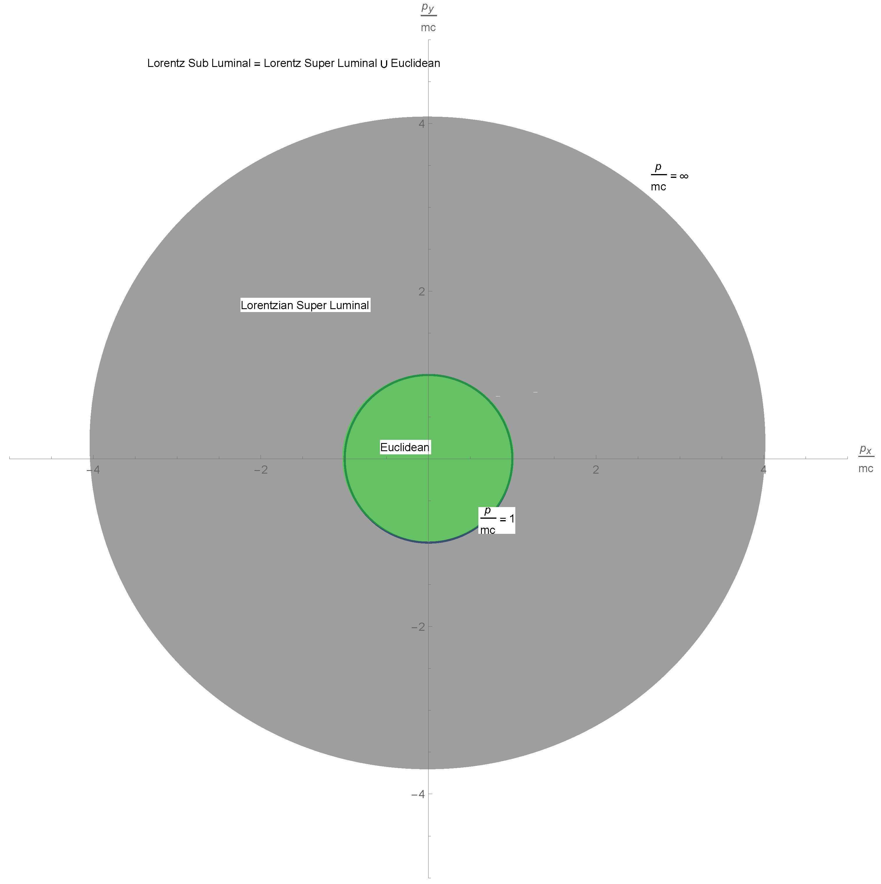
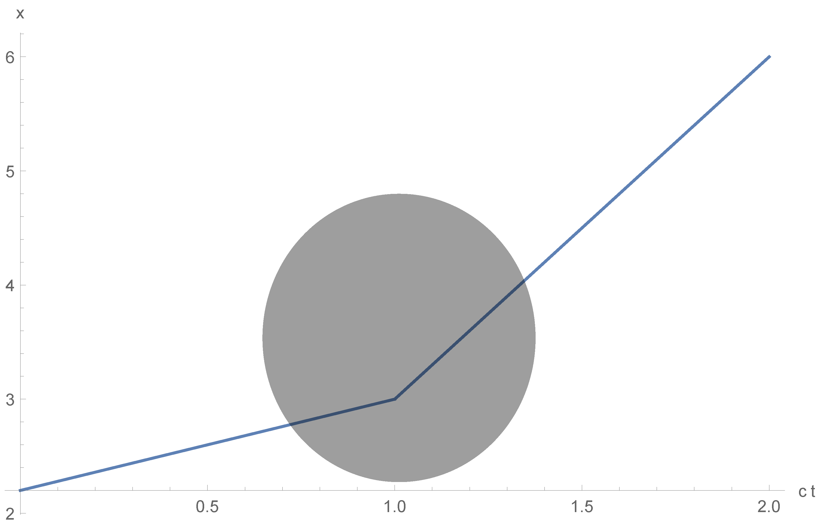
Another obvious physical implication of the previous analysis involve a far fetched technological scenario, in which a particle is accelerated to a velocity close to the velocity c in a Lorentz space-time, enters into an artificially created Euclidean space-time and accelerated further in this region to velocities above the speed c, and finally emerges in a Lorentz space in which it will remain above the speed c for ever unless it is decelerated in an Euclidean space again (see Figure 24). This may happen to a particle that travels radially in a Friedman–Lemaitre–Robertson–Walker metric passing outwards the critical radius of $r_c=\frac{1}{\sqrt{\kappa }}$ and then coming back at superluminal velocities. However, this will be very difficult to do artificially. Obviously a metric change will require a significant $T_{\mu \nu }$ according to Equation (1). Taking into account that the largest metric deviation from the Lorentzian metric is the solar system on the surface of the sun in $h_{00}\sim {10}^{-6}$ [37], it does not seem conceivable that such a metric change can be indeed implemented.

Finally, one should take into account that although classical physics is assumed to occur in a Lorentzian metric, quantum field theory calculations are done frequently in an Euclidean background using the rotation of Wick. This is explained through the concept of analytic continuation. However, this procedure is a mathematical technique that has no physical reason in a Lorentzian space-time but may make perfect sense if it is part of space-time, in particular if the part that is very near to the said particle is Euclidean. Hence, one may speculate that each elementary particle may carry with it a “bubble” of a microscopic Euclidean space-time, which may be considered as a one-dimensional string or vortex when viewed from a four-dimensional space-time perspective.

6. Conclusions

GR allows for non-Lorentzian space-times; this is in particular allowed in part of the Friedman–Lemaitre–Robertson–Walker universe. Thus, superluminal particles can exist in such a cosmology. Some of the cosmological consequences of superluminal particles for the homogeneity problem and dark energy problems are briefly described. Some implications of non Lorentzian metrics not connected to superluminality but that may result from non-Euclidean metrics are suggested. Much more detailed analysis is needed to reach a definite conclusion regarding each of the above physical problems. However, the existence of non-Lorentzian space-times and, as a consequence (not an additional assumption), superluminal particles, suggests a possible solution. Of course, just having a rapid expansion in this case does not make inflation in the early universe redundant, and much more detailed and rigorous studies are needed, in particular with respect to the CMB spatial spectrum and the evolution of large scale structure in the universe.

In the scope of the current paper we have only considered canonical ensembles in the number of particles to be fixed, however, at high energies pair creation from the vacuum is possible. Hence, a grand canonical ensemble should be studied. Quantum mechanical effects were also out of the scope of the current paper, which concentrated on classical effects only.

Finally, an Euclidean metric will effect the energy momentum tensor, thus affecting the allowed solutions of the Friedman–Lemaitre–Robertson–Walker universe. A derivation of an exact mathematical model describing the transition from the Euclidean to the Lorentzian universe in which we live in, is left for future studies.

References

1. Weinberg, S. Gravitation and Cosmology: Principles and Applications of the General Theory of Relativity; John Wiley & Sons, Inc.: Hoboken, NJ, USA, 1972. [Google Scholar]
2. Yahalom, A. The Geometrical Meaning of Time. Found. Phys. 2008, 38, 489–497. [Google Scholar] [CrossRef]
3. Yahalom, A. Gravity and Faster than Light Particles. J. Mod. Phys. 2013, 4, 1412–1416. [Google Scholar] [CrossRef] [Green Version]
4. Eddington, A.S. The Mathematical Theory of Relativity; Cambridge University Press: Cambridge, UK, 1923. [Google Scholar]
5. Carlini, A.; Greensite, J. Why is spacetime Lorentzian? Phys. Rev. D 1994, 49, 2. [Google Scholar] [CrossRef] [Green Version]
6. Elizalde, E.; Odintsov, S.D.; Romeo, A. Dynamical determination of the metric signature in spacetime of non-trivial topology. Class. Quantum Gravity 1994, 11, L61–L67. [Google Scholar] [CrossRef] [Green Version]
7. Itin, Y.; Hehl, F.W. Los Alamos Archive gr-qc/0401016. 6 January 2004. Available online: https://arxiv.org/abs/gr-qc/0401016 (accessed on 10 October 2007).
8. van Dam, H.; Ng, Y.J. Los Alamos Archive hep-th/0108067. 10 August 2001. Available online: https://arxiv.org/abs/hep-th/0108067 (accessed on 10 October 2007).
9. Yahalom, A. The Gravitational Origin of the Distinction between Space and Time. Int. J. Mod. Phys. D 2009, 18, 2155–2158. [Google Scholar] [CrossRef]
10. Yahalom, A. Advances in Classical Field Theory; Bentham eBooks: Sharjah, United Arab Emirates, 2011; Chapter 6; ISBN 978-1-60805-195-3. [Google Scholar]
11. Yahalom, A. On the Difference between Time and Space. Cosmology 2014, 18, 466–483. [Google Scholar]
12. Yahalom, A. Gravity, Stability and Cosmological Models. Int. J. Mod. Phys. D 2017, 26, 1743026. [Google Scholar] [CrossRef]
13. Yourgrau, P. A World without Time; Basic Books: New York, NY, USA, 2006. [Google Scholar]
14. Yahalom, A. Gravity and the Complexity of Coordinates in Fisher Information. Int. J. Mod. Phys. D 2010, 19, 2233–2237. [Google Scholar] [CrossRef]
15. Christodoulou, D.; Klainerman, S. The Global Nonlinear Stability of the Minkowski Space; Princeton University Press: Princeton, NJ, USA, 1993. [Google Scholar]
16. Narlikar, J.V. Introduction to Cosmology; Cambridge University Press: Cambridge, UK, 1993. [Google Scholar]
17. Guth, A.H. Inflationary universe: A possible solution to the horizon and flatness problems. Phys. Rev. D 1981, 23, 347. [Google Scholar] [CrossRef] [Green Version]
18. Linde, A. A new inflationary universe scenario. Phys. Lett. B 1982, 108, 389. [Google Scholar] [CrossRef]
19. Linde, A. Chaotic inflation. Phys. Lett. B 1983, 129, 177. [Google Scholar] [CrossRef]
20. Ade, P.A.R. et al. [BICEP2 Collaboration] Detection of B-Mode Polarization at Degree Angular Scales by BICEP2. Phys. Rev. Lett. 2014, 112, 241101. [Google Scholar] [CrossRef] [Green Version]
21. Sakharov, A.D. Cosmological transitions with changes in the signature of the metric. Sov. Phys. JETP 1984, 60, 214–218. Available online: http://jetp.ras.ru/cgi-bin/e/index/e/60/2/p214?a=list (accessed on 1 February 2022).
22. Shestakova, T.P. The Birth of the Universe as a Result of the Change of the Metric Signature. Physics 2022, 4, 160–171. [Google Scholar] [CrossRef]
23. Hartle, J.B.; Hawking, S.W. Wave function of the Universe. Phys. Rev. D 1983, 28, 2960–2975. [Google Scholar] [CrossRef]
24. Ellis, G.; Sumeruk, A.; Coule, D.; Hellaby, C. Change of signature in classical relativity. Class. Quantum Gravity 1992, 9, 1535–1554. [Google Scholar] [CrossRef]
25. Vilenkin, A. Birth of inflationary universes. Phys. Rev. D 1983, 27, 2848–2855. [Google Scholar] [CrossRef]
26. Altshuler, B.L. Andrei Sakharov’s research work and modern physics. Physics-Uspekhi 2021, 64, 427–451. [Google Scholar] [CrossRef]
27. Altshuler, B.L.; Barvinsky, A.O. Quantum cosmology and physics of transitions with a change of the spacetime signature. Physics-Uspekhi 1996, 39, 429–460. [Google Scholar] [CrossRef]
28. Zhang, F. Alternative route towards the change of metric signature. Phys. Rev. D 2019, 100, 064043. [Google Scholar] [CrossRef] [Green Version]
29. Bojowald, M.; Brahma, S. Loop quantum gravity, signature change, and the no-boundary proposal. Phys. Rev. D 2020, 102, 106023. [Google Scholar] [CrossRef]
30. Davidson, A.; Yellin, B. Is spacetime absolutely or just most probably Lorentzian? Class. Quantum Gravity 2016, 33, 165009. [Google Scholar] [CrossRef]
31. Gover, A.; Faingersh, A.; Eliran, A.; Volshonok, M.; Kleinman, H.; Wolowelsky, S.; Kapilevich, B.; Lasser, Y.; Seidov, Z.; Kanter, M.; et al. Radiation Measurements in the New Tandem Accelerator FEL. Nucl. Instrum. Methods 2004, 528, 23–27. [Google Scholar] [CrossRef] [Green Version]
32. Balal, N.; Magori, E.; Yahalom, A. Design of a Permanent Magnet Wiggler for a THz Free Electron Laser. Acta Phys. Pol. A 2015, 128, 259–263. [Google Scholar] [CrossRef]
33. Jackson, J.D. Classical Electrodynamics, 3rd ed.; Wiley: New York, NY, USA, 1999. [Google Scholar]
34. Walecka, J.D. Fundamental Statistical Mechanics, Manuscript and Notes of Felix Bloch; Imperial College Press & World Scientific: London, UK, 2000. [Google Scholar]
35. Guth, A.H. Starting the universe: The Big Bang and cosmic inflation. In Bubbles, Voids and Bumps in Time: The New Cosmology; Cornell, J., Ed.; Cambridge University Press: Cambridge, UK, 1995; p. 105. [Google Scholar]
36. Peebles, P.J.E.; Ratra, B. The Cosmological Constant and Dark Energy. Rev. Mod. Phys. 2003, 75, 559–606. [Google Scholar] [CrossRef] [Green Version]
37. Yahalom, A. Lensing Effects in Retarded Gravity. Symmetry 2021, 13, 1062. [Google Scholar] [CrossRef]
Figure 1. Free momentum for Lorentzian subluminal particles, the correct expression is compared to the classical one. The blue line is the correct expression while the orange line is the classical approximation.
Universe 08 00594 g001
Figure 2. Free momentum for Euclidean subluminal particles, the correct expression is compared to the classical one. The blue line is the correct expression while the orange line is the classical approximation.
Universe 08 00594 g002
Figure 3. Free momentum for Euclidean particles.
Universe 08 00594 g003
Figure 4. Free momentum for Lorentzian superluminal particles.
Universe 08 00594 g004
Figure 5. A depiction of the cross section of the momentum space for the cases considered: Euclidean (a compact sphere) in green, Lorentzian superluminal (an infinite domain with a spherical hall) in gray, and Lorentzian subluminal (the entire momentum plane). The latter is a union of the former.
Universe 08 00594 g005
Figure 6. Kinetic energy for Lorentzian subluminal particles, the correct expression is compared with the classical one. The blue line is the correct expression while the orange line is the classical approximation.
Universe 08 00594 g006
Figure 7. Kinetic energy for Euclidean particles, the correct expression (blue) is compared with the classical approximation (orange).
Universe 08 00594 g007
Figure 8. Kinetic energy for Euclidean particles of subluminal and superluminal velocities.
Universe 08 00594 g008
Figure 9. Kinetic energy for Lorentzian particles of superluminal velocities.
Universe 08 00594 g009
Figure 10. Partition function for a free subluminal Lorentzian particle, the blue line is the correct value while the orange represents the low velocity approximation.
Universe 08 00594 g010
Figure 11. Probability density function for a free subluminal Lorentzian particle as function of p and λ .
Universe 08 00594 g011
Figure 12. Probability density function for a free subluminal Lorentzian particle as function of p for λ = 1 . The blue line depicts the correct value, while the orange line depicts the Maxwell–Boltzmann approximation.
Universe 08 00594 g012
Figure 13. Probability density function for a free subluminal Lorentzian particle as function of p for λ = 50 . The blue line depicts the correct value, while the orange line depicts the Maxwell–Boltzmann approximation.
Universe 08 00594 g013
Figure 14. Average energy for free Lorentzian subluminal particles with high λ . The blue line depicts the correct value, while the orange line depicts the Maxwell–Boltzmann approximation.
Universe 08 00594 g014
Figure 15. Average energy for free Lorentzian subluminal particles with low λ . The blue line depicts the correct value, while the orange line depicts the Maxwell–Boltzmann approximation.
Universe 08 00594 g015
Figure 16. Partition function for a free Euclidean particle.
Universe 08 00594 g016
Figure 17. Probability density function for a free Euclidean particle as function of p and λ .
Universe 08 00594 g017
Figure 18. Probability density function for a free Euclidean particle as function of p for λ = 5 .
Universe 08 00594 g018
Figure 19. Average energy for free Euclidean particles with high λ .
Universe 08 00594 g019
Figure 20. Partition function for a free superluminal Lorentzian particle.
Universe 08 00594 g020
Figure 21. Probability density function for free superluminal Lorentzian particle as a function of p and | λ | .
Universe 08 00594 g021
Figure 22. Probability density function for a free superluminal Lorentzian particle as a function of p for | λ | = 1 .
Universe 08 00594 g022
Figure 23. Average energy for free Lorentzian subluminal particles with high | λ | .
Universe 08 00594 g023
Figure 24. A schematic acceleration scheme of a particle in an Euclidean portion of space-time.
Universe 08 00594 g024
Publisher’s Note: MDPI stays neutral with regard to jurisdictional claims in published maps and institutional affiliations.