


A Reanalysis of the Latest SH0ES Data for H0: Effects of New Degrees of Freedom on the Hubble Tension


Abstract
:1. Introduction
1.1. The Current Status of the Hubble Tension and Its Four Assumptions
- There are no significant systematic errors in the measurements of the properties (period, and metallicity) and luminosities of Cepheid calibrators and SnIa.
- The physical laws involved and the calibration properties of Cepheids and SnIa in all the rungs of the distance ladder are well understood and modeled properly.
- The scale of the sound horizon at the last scattering surface is the one calculated in the context of the standard cosmological model with the known degrees of freedom (cold dark matter, baryons and radiation) and thus, it is a reliable distance calibrator.
1.2. The New SH0ES Cepheid+SnIa Data
1.3. The Prospect of New Degrees of Freedom in the SH0ES Data Analysis
- There are no significant systematics in the SH0ES data, and thus they are reliable.
- The CMB sound horizon scale used as a calibrator in the inverse distance ladder approach is correctly obtained in the standard model using the known particles.
- The Hubble expansion history from the time of recombination up to (or even ) used in the inverse distance ladder measurement of is provided correctly by the standard Planck18CDM cosmological model.
- How can new degrees of freedom (new parameters) be included in the SH0ES data analysis for the determination of ?
- What are the new degrees of freedom that can expose internal tensions and inhomogeneities in the Cepheid/SnIa data?
- What new degrees of freedom can lead to a best-fit value of that is consistent with Planck?
2. The New SH0ES Data and Their Standard Analysis: Hints for Intrinsic Tensions
2.1. The Original Baseline SH0ES Analysis: A Comprehensive Presentation
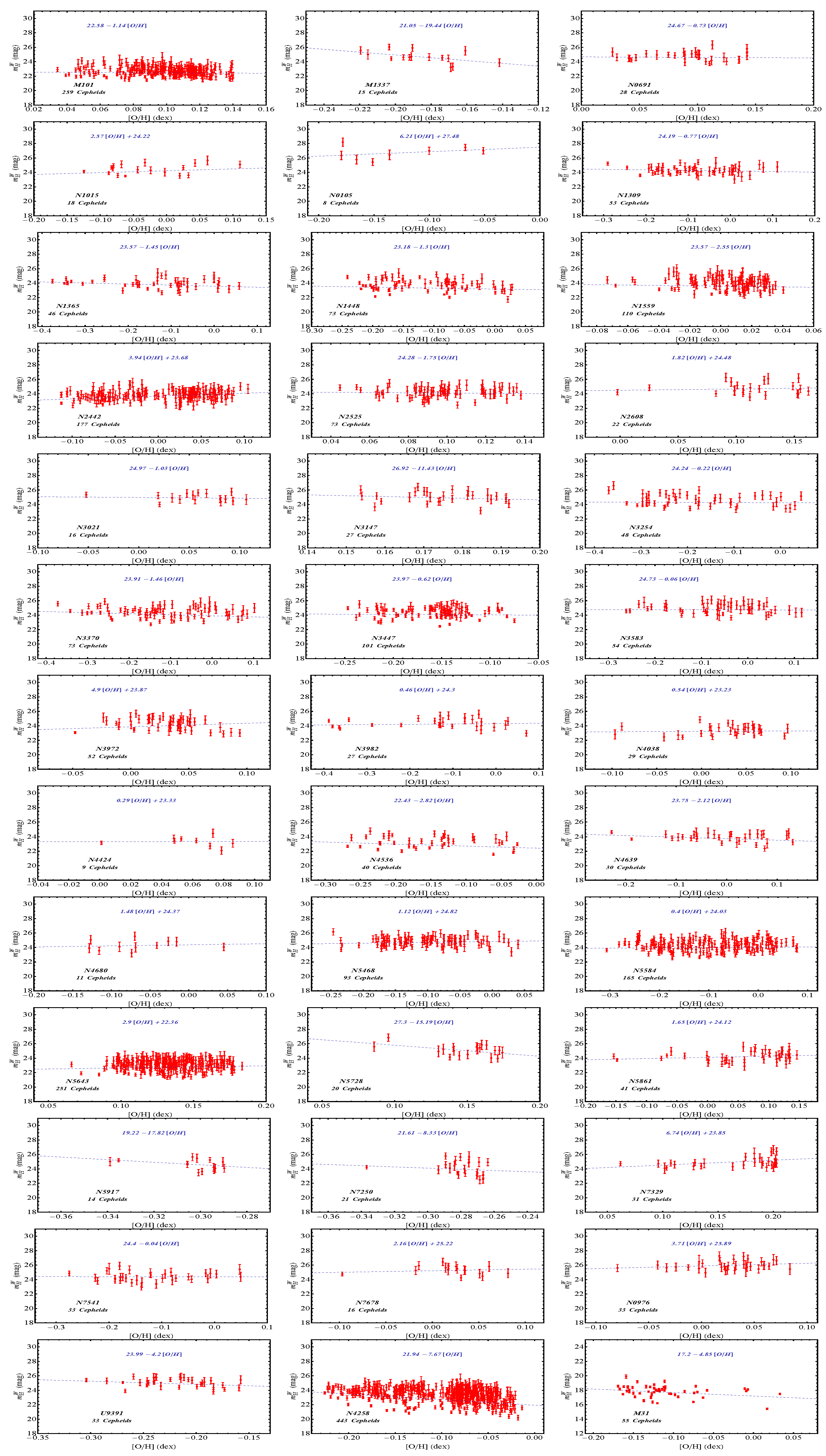
- The equation that connects the measured Wesenheit magnitude of the jth Cepheid in the ith galaxy with the host distance moduli and the modeling parameters , and is of the following form6where is the inferred distance modulus to the galaxy, is the zeropoint Cepheid absolute magnitude of a period Cepheid (d for days), and − are the slope parameters that represent the dependence of magnitude on both period and metallicity. The is a measure of the metallicity of the Cepheid. The usual bracket shorthand notation for the metallicity represents the Cepheid metal abundance compared to that of the SunHere, O and H are the number of oxygen and hydrogen atoms per unit of volume, respectively. The unit often used for metallicity is the dex (decimal exponent) defined as . Additionally, the bracket shorthand notation for the period is used as (P in units of days)
- The color- and shape-corrected SnIa B-band peak magnitude in the ith host is connected with the distance modulus of the ith host and with the SnIa absolute magnitude as shown in Equation (5), i.e.,The distance modulus is connected with the luminosity distance in aswhere in a flat universewhere is the Hubble free luminosity distance, which is independent of .
- Using Equations (9)–(11), it is easy to show that that is connected with the SnIa absolute magnitude and the Hubble free luminosity distance asIn the context of the cosmographic expansion of valid for , we havewhere and are the deceleration and jerk parameters, respectively. Thus, Equations (12) and (13) lead to the equation that connects with the SnIa absolute magnitude , which may be expressed aswhere we have introduced the parameter as defined in the SH0ES analysis [153].
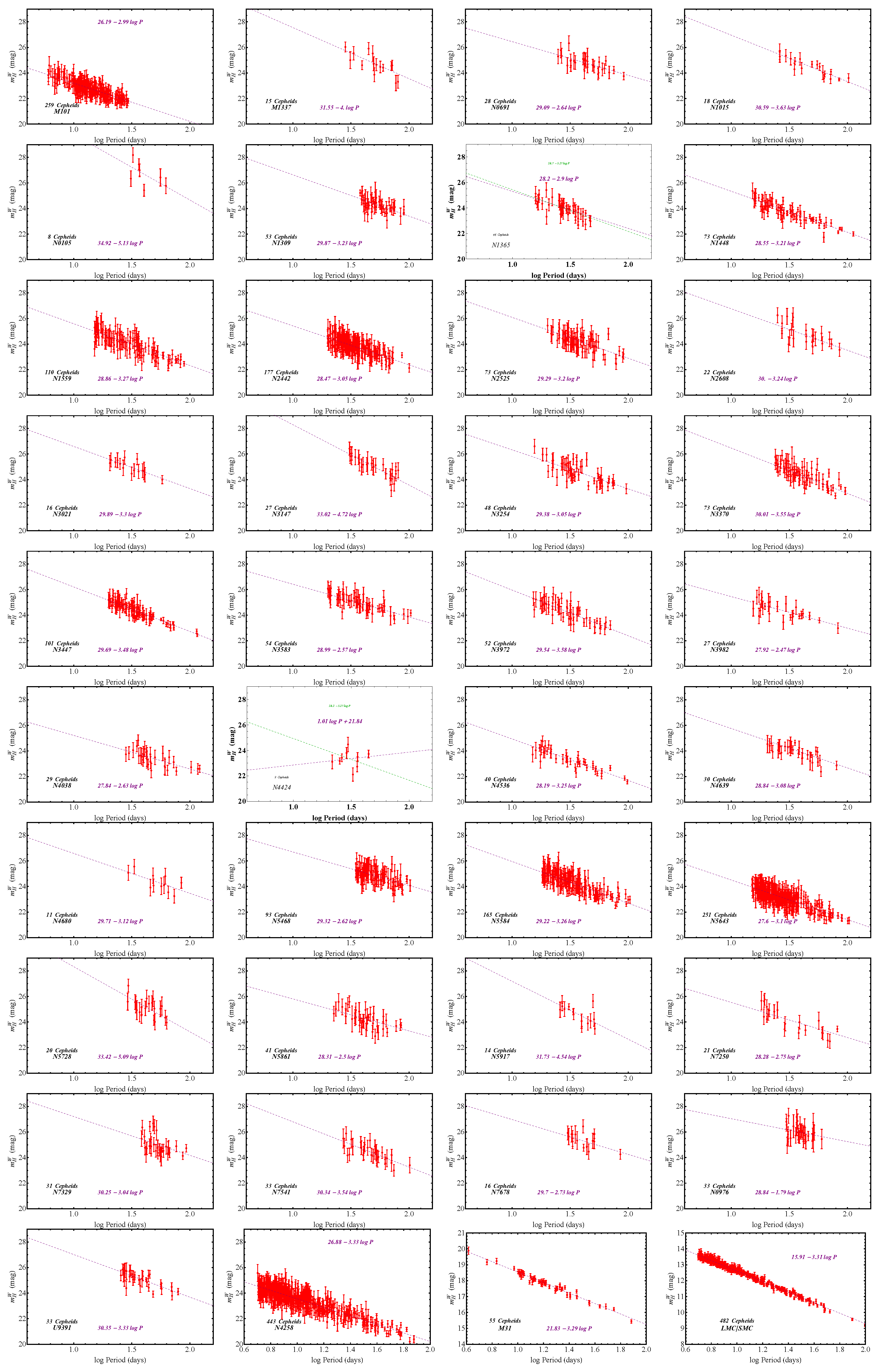
- The Cepheid Wesenheit magnitudes are presented as residuals with respect to a fiducial P-L term aswhere is a fiducial Cepheid P-L slope. As a result of this definition, the derived best-fit slope is actually a residual slope .
- The residual Cepheid Wesenheit magnitudes of the Cepheids in the anchors N4258, LMC and the supporting pure Cepheid host SMC (non SnIa hosts), are presented after subtracting a corresponding fiducial distance modulus obtained with geometric methods7.
- The SnIa standardized apparent magnitudes in the Hubble flow are presented as residuals after subtracting the Hubble free luminosity distance with cosmographic expansion (see Equation (13)).
 |
| q = | 47 parameters |
 |
- The number of entries of the parameter vector is 47 and not 46 as implied in R21 due to the extra dummy parameter X, which is included in the released data , and but not mentioned in R21.
- The entry referred as in R21 in the parameter vector should be because it is actually the residual () as stated above and not the original slope of the P-L relation (its best-fit value is ).
- The number of constraints shown in the definition of the vector in R21 is five, while in the actual released data , and , we found the eight constraints defined above.
2.2. Homogeneity of the Cepheid Modeling Parameters
3. Generalized Analysis: New Degrees of Freedom Allowing for a Physics Transition
3.1. Allowing for a Transition of a Cepheid Calibration Parameter
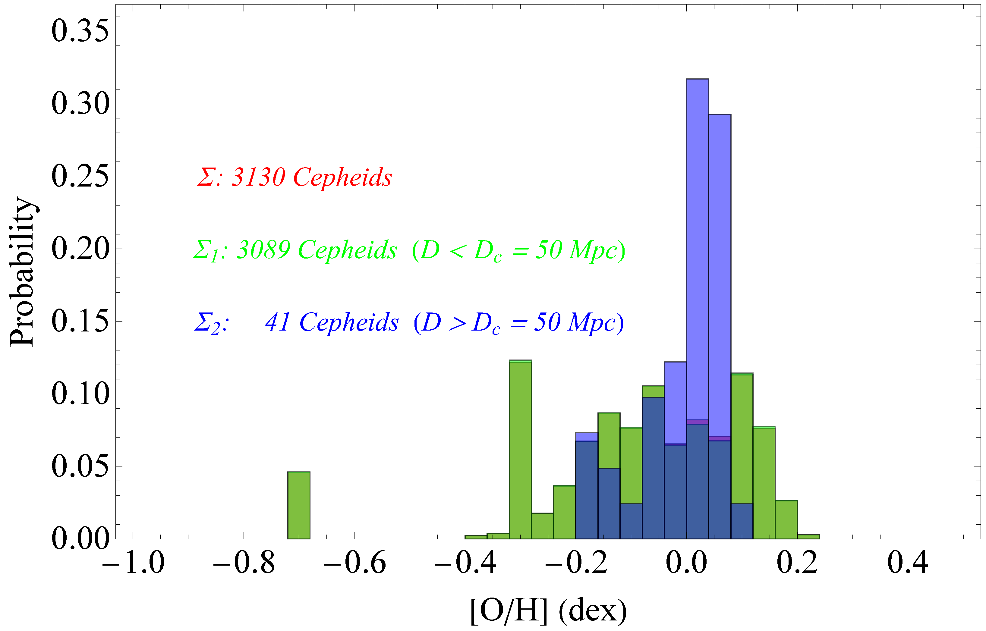
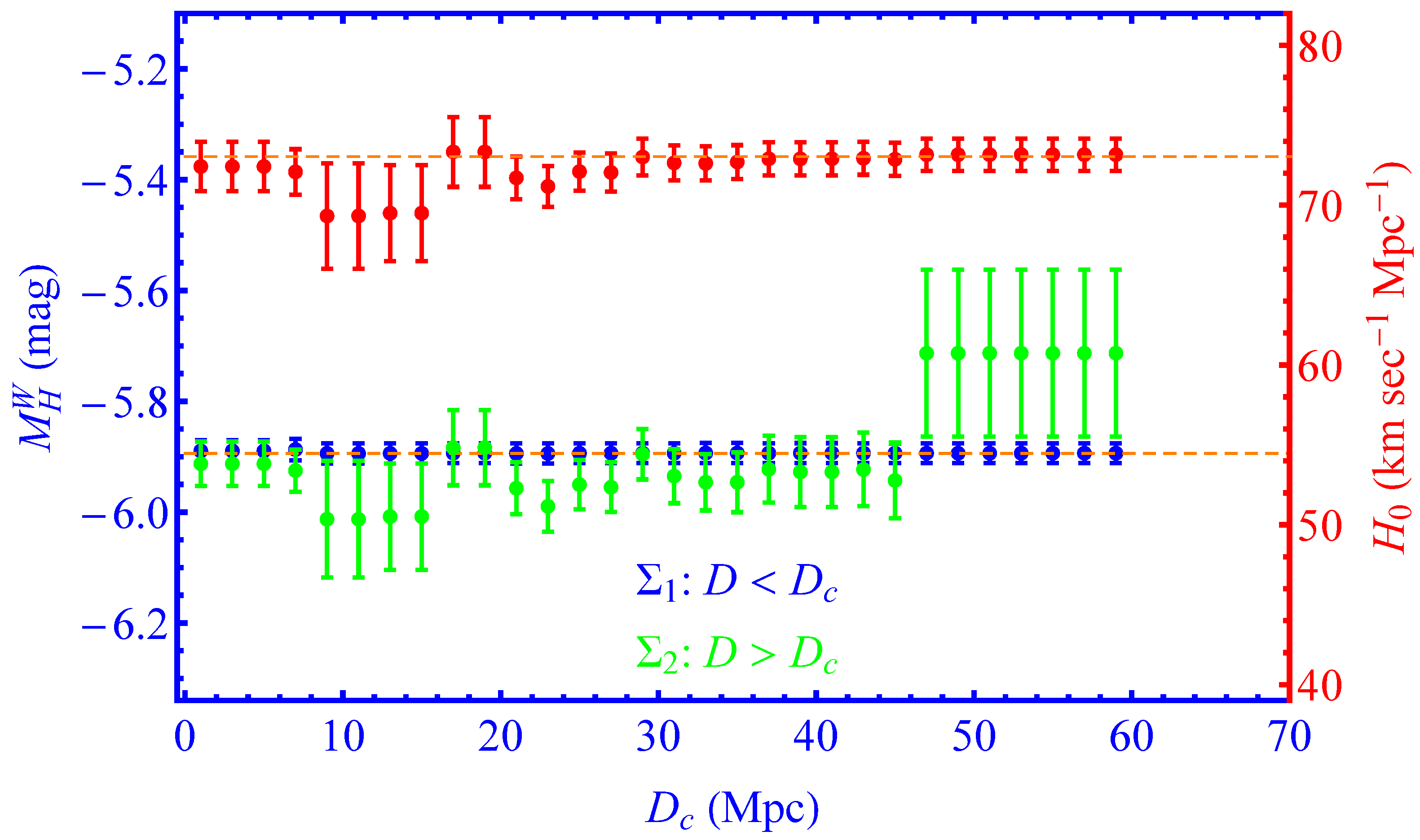
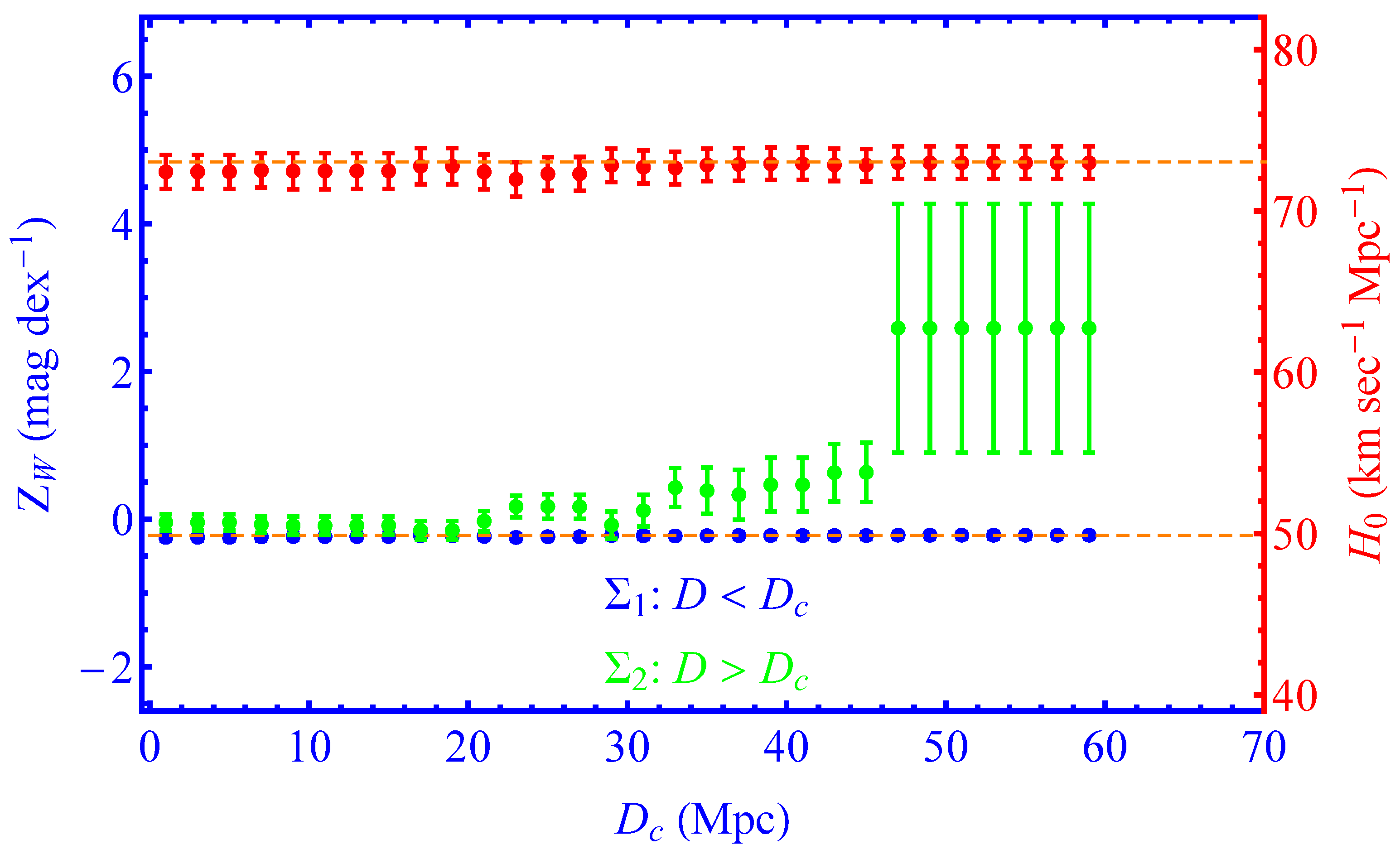
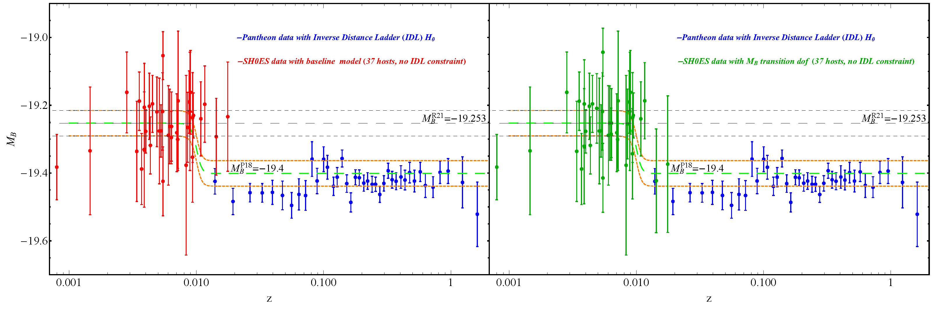
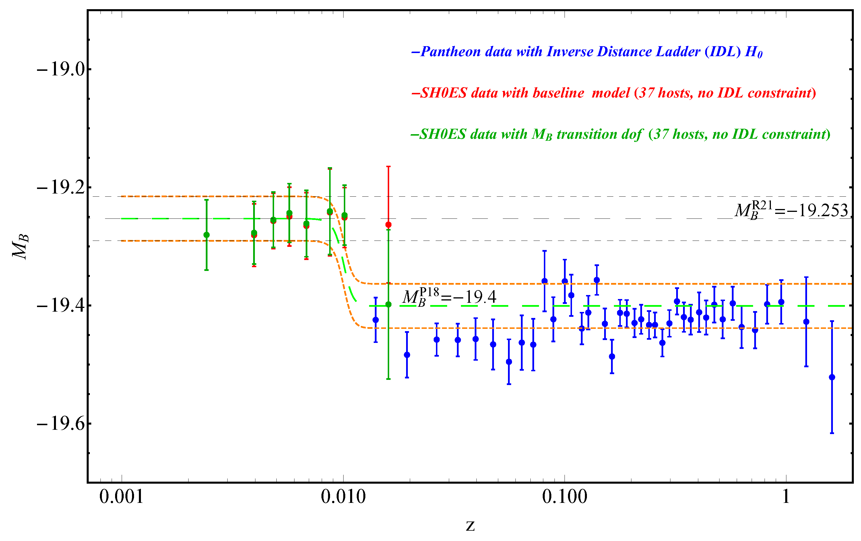
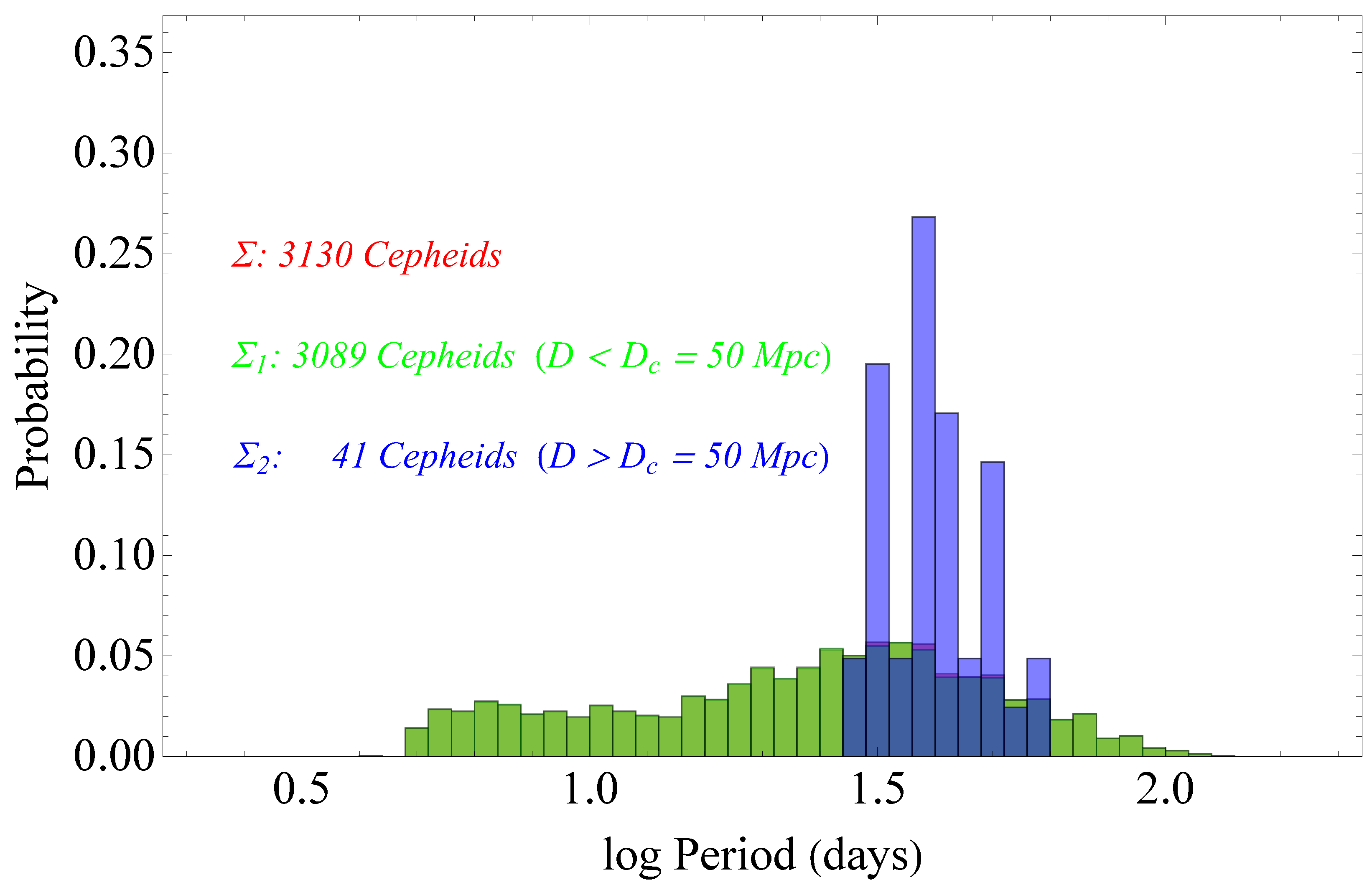
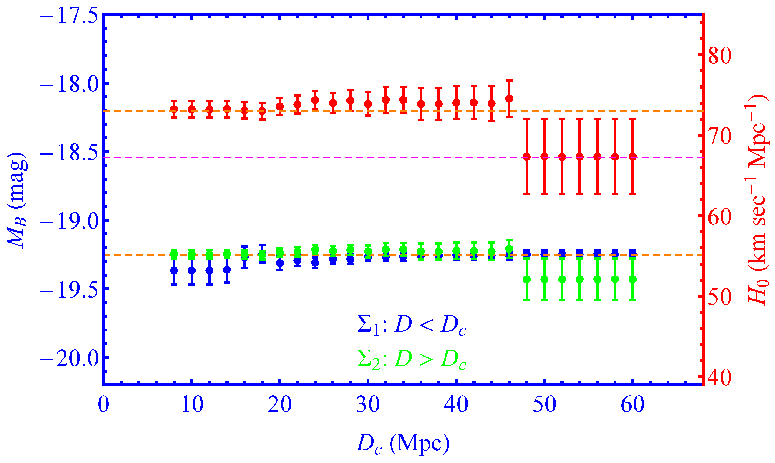
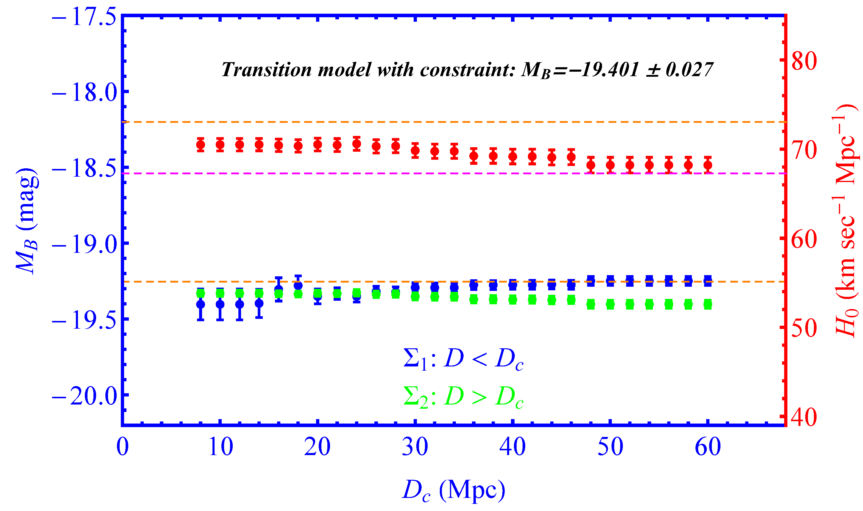
- When the SnIa absolute magnitude is allowed to change at ( transition) and for , the best-fit value of drops spontaneously to the best-fit Planck18/CDM value, albeit with larger uncertainty (see Figure 8 and second row of Table 4). This remarkable result appears with no prior or other information from the inverse distance ladder results. Clearly, there are increased uncertainties of the best-fit parameter values for this range of because the most distant usable Cepheid hosts are at distances Mpc (N7329), Mpc (N0976) and Mpc (N0105) and only two of them are at distance beyond 47 Mpc. These hosts (N0975 and N0105) have a total of 41 Cepheids and 4 SnIa. Due to the large uncertainties involved, there is a neutral model preference for this transition degree of freedom at Mpc (the small drop of by is balanced by the additional parameter of the model). This, however, changes dramatically if the inverse distance ladder constraint on is included in the vector as discussed below.
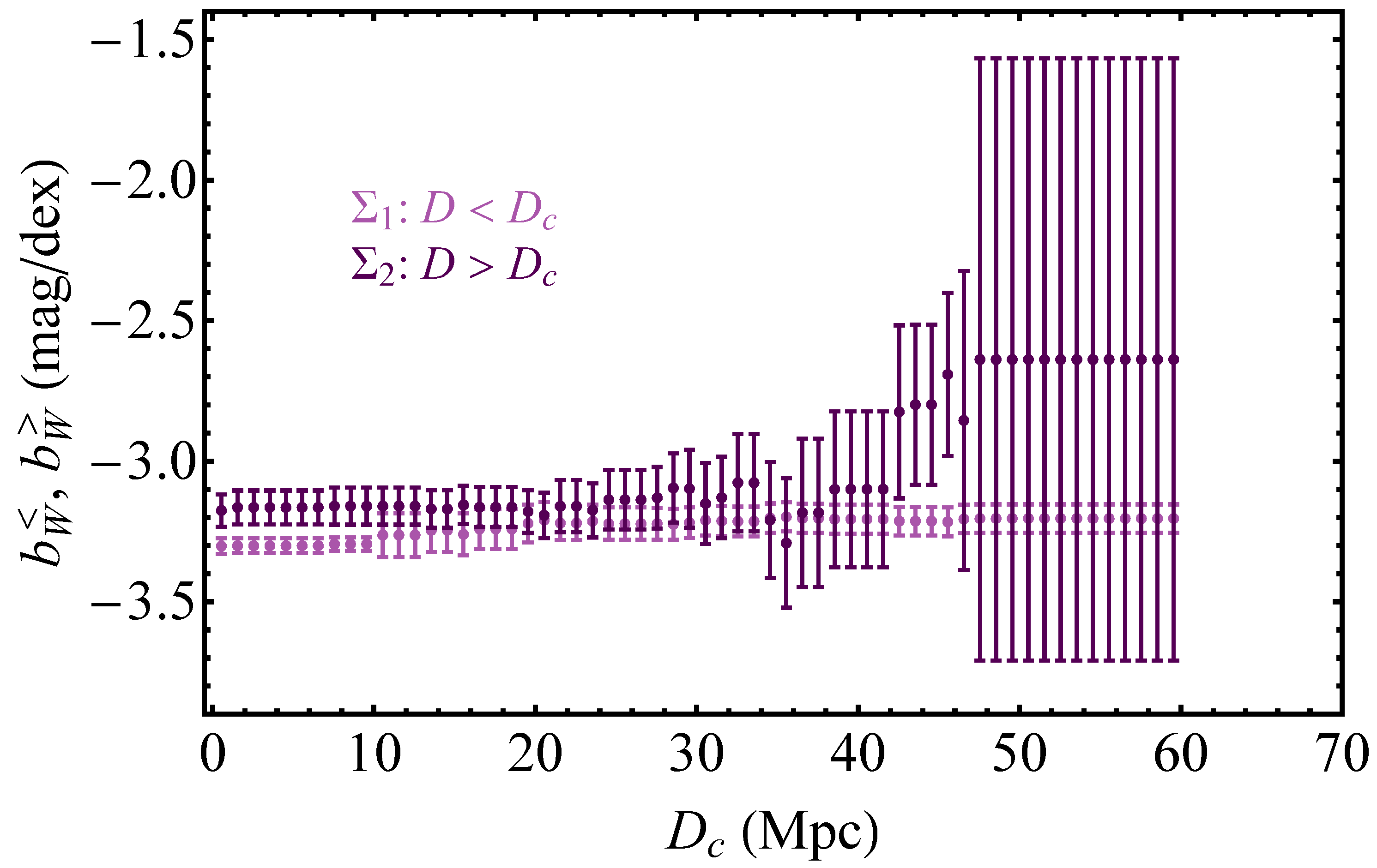
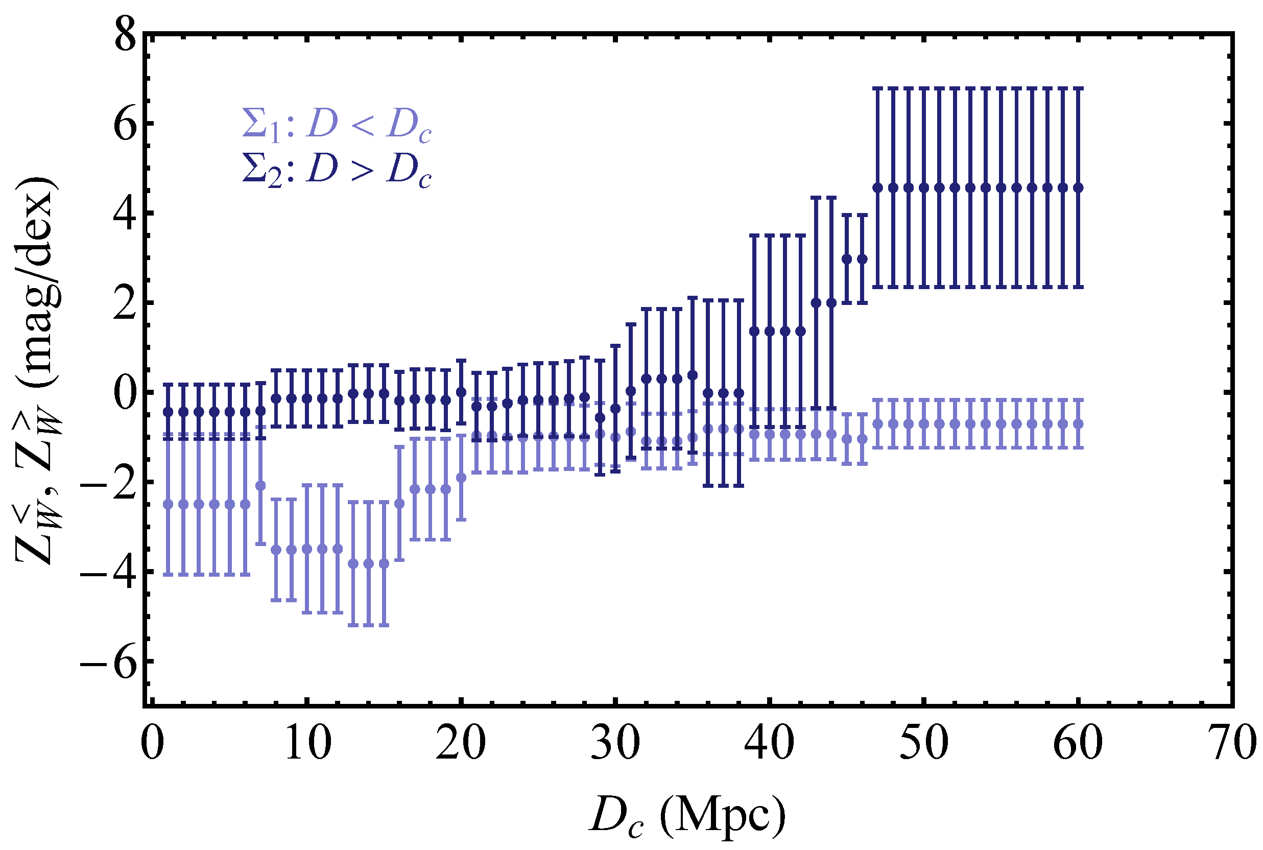
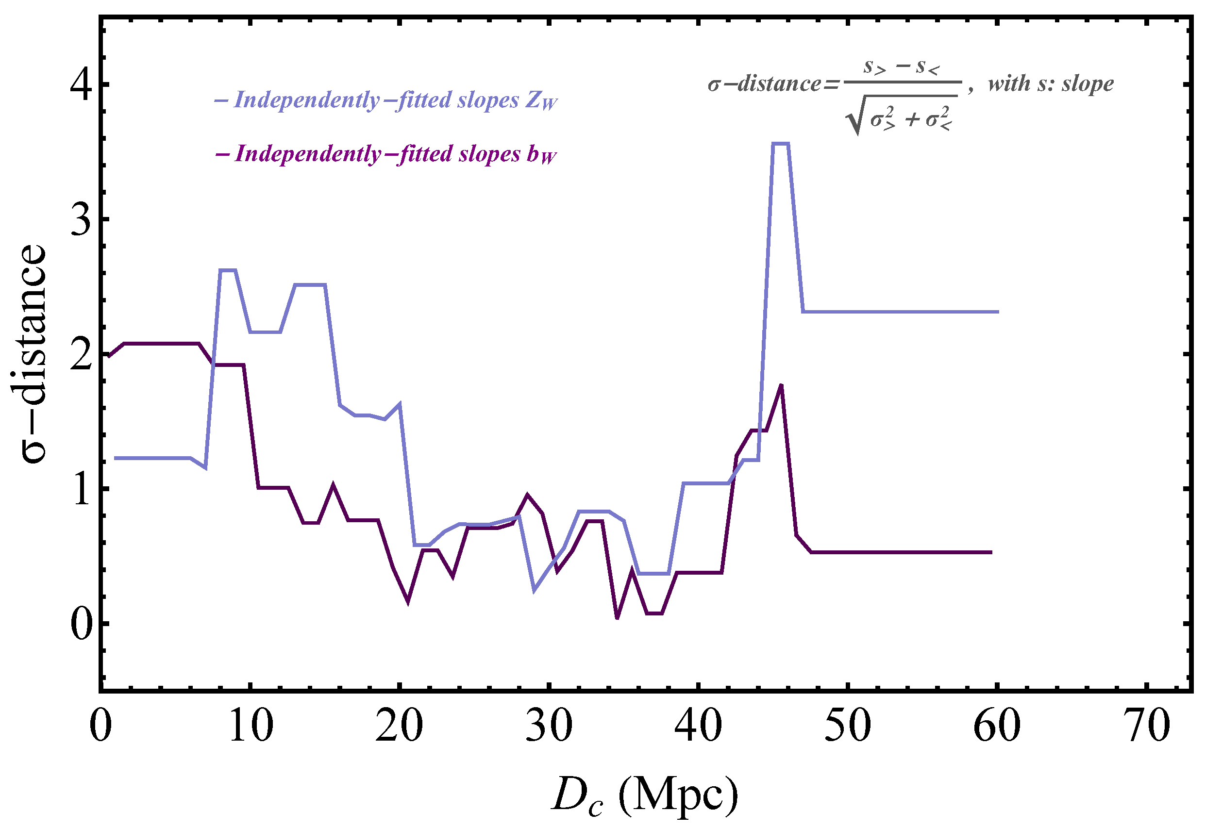
- For all four modeling parameters considered, there is a sharp increase in the absolute difference between the high–low-distance best-fit parameter values for Mpc. The statistical significance of this split, however, is low due to the relatively small number of available Cepheids at Mpc.
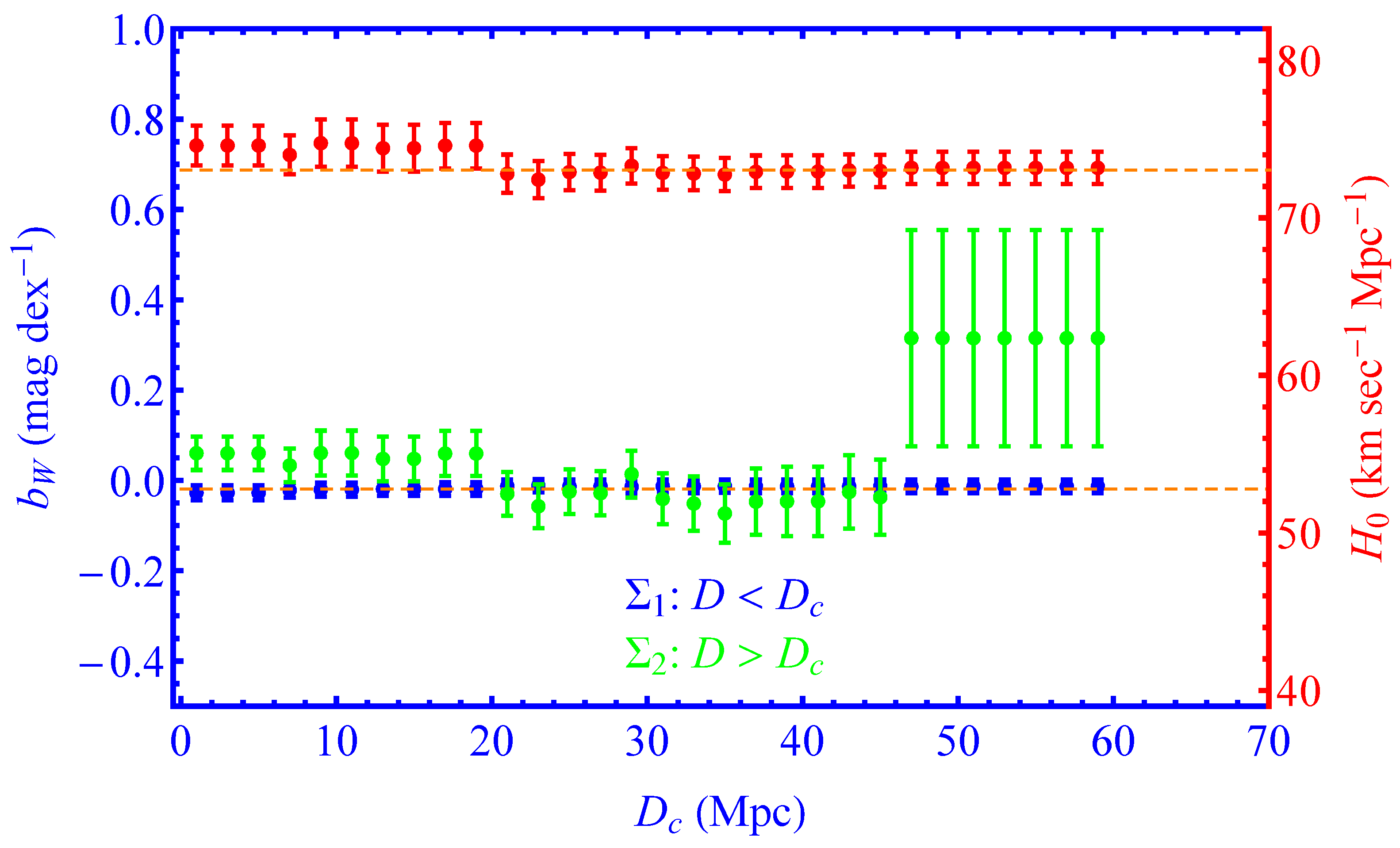
- The best-fit value of changes significantly when the SnIa absolute magnitude is allowed to make a transition at Mpc but is not significantly affected if the three Cepheid modeling parameters , and are allowed to make a transition at any distance. This is probably due to the large uncertainties involved and due to the fact that is only indirectly connected with the three Cepheid modeling parameters.
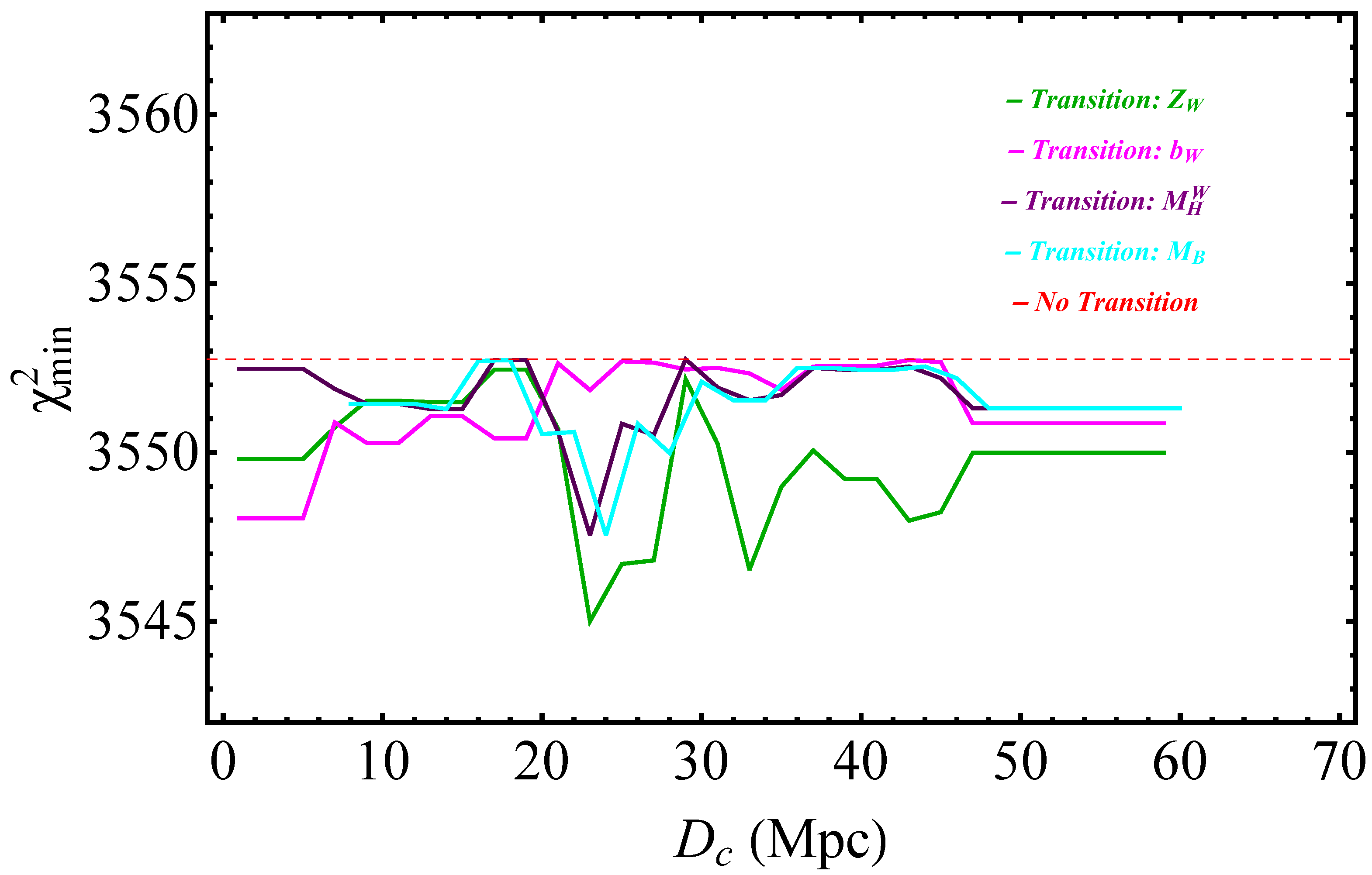
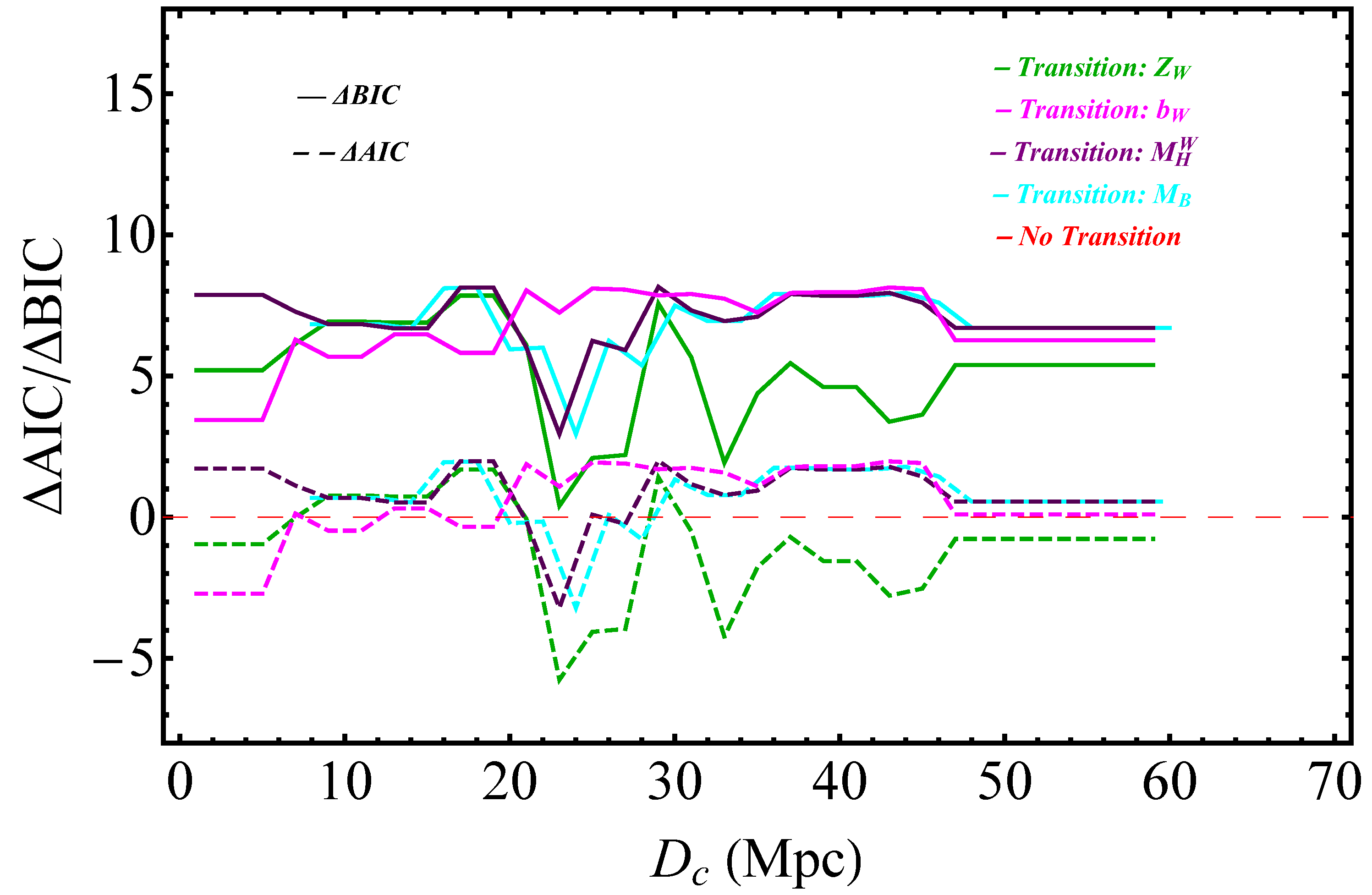
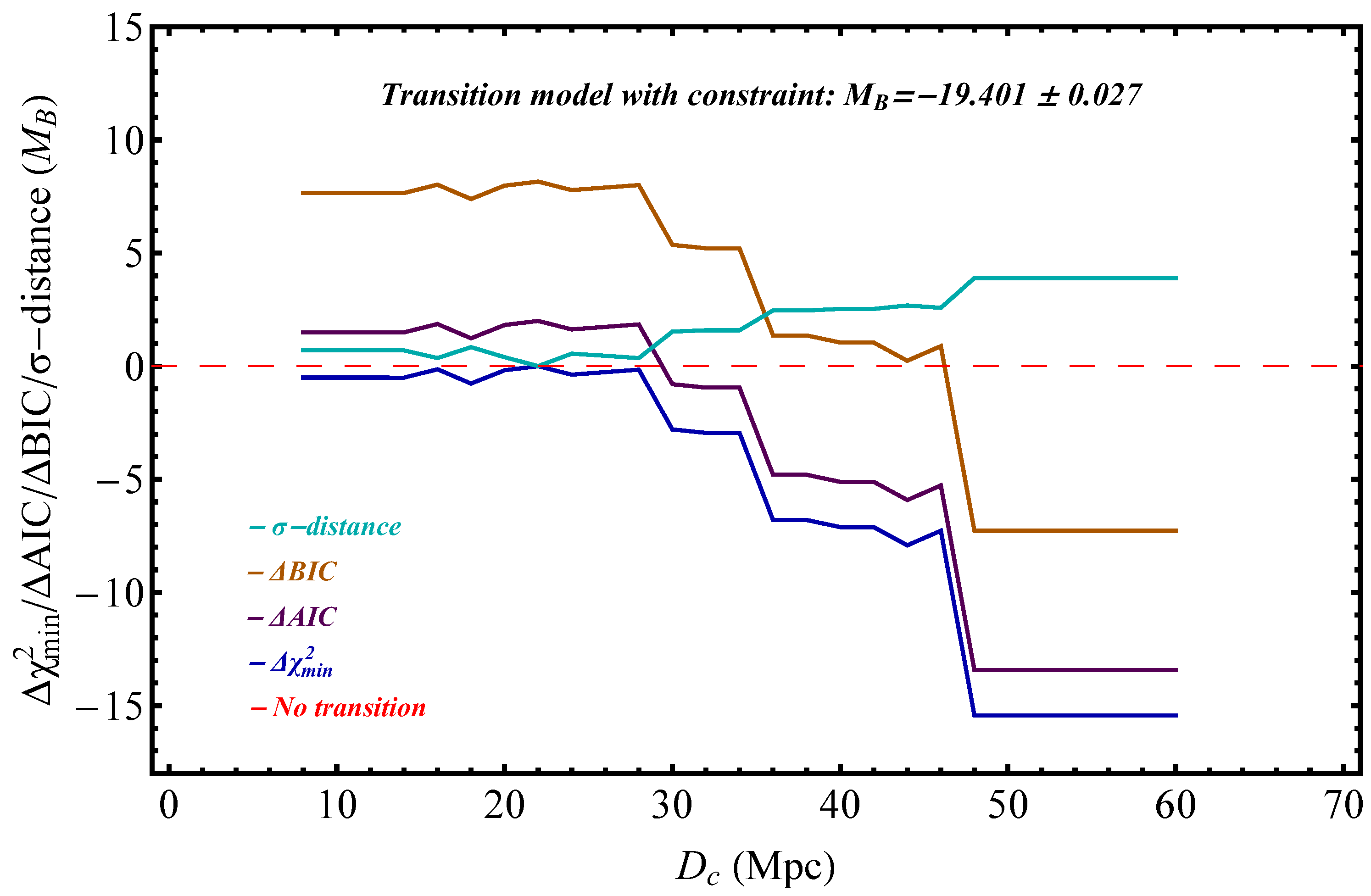
- Each one of the transition degrees of freedom mildly reduces , thus improving the fit to the data, but these transition models are not strongly preferred by the model selection criteria, which penalize the extra parameter implied by these models. This is demonstrated in Figure 12 and Figure 13, which show the values of , and of the four transition models with respect to the baseline SH0ES model for various transition distances. As discussed below, this changes dramatically if the inverse distance ladder constraint on is introduced in the analysis.
3.2. The Effect of the Inverse Distance Ladder Constraint
How does the level of preference for the transition model (compared to the SH0ES baseline model) change if an additional constraint is included in the analysis obtained from the inverse distance ladder best fit for ?
- In the presence of the inverse distance ladder constraint, the model with the transition degree of freedom at Mpc is strongly preferred over the baseline model as indicated by the model selection criteria, despite the additional parameter it involves (comparison of the last two rows of Table 4).
- The transition degree of freedom, when allowed in each of the other three modeling parameters, does not lead to a spontaneous resolution of the Hubble tension since the best-fit value of is not significantly affected. However, it does induce an increased absolute difference between the best-fit values of the high-distance and low-distance parameters, which, however, is not statistically significant due to the large uncertainties of the bin with Mpc (see also Figure 9, Figure 10 and Figure 11).
4. Conclusions
Author Contributions
Funding
Data Availability Statement
Acknowledgments
Conflicts of Interest
Appendix A. Covariance Matrix
 |
Appendix B. Analytic Minimization of χ 2
Appendix C. Reanalysis of Individual Cepheid Slope Data
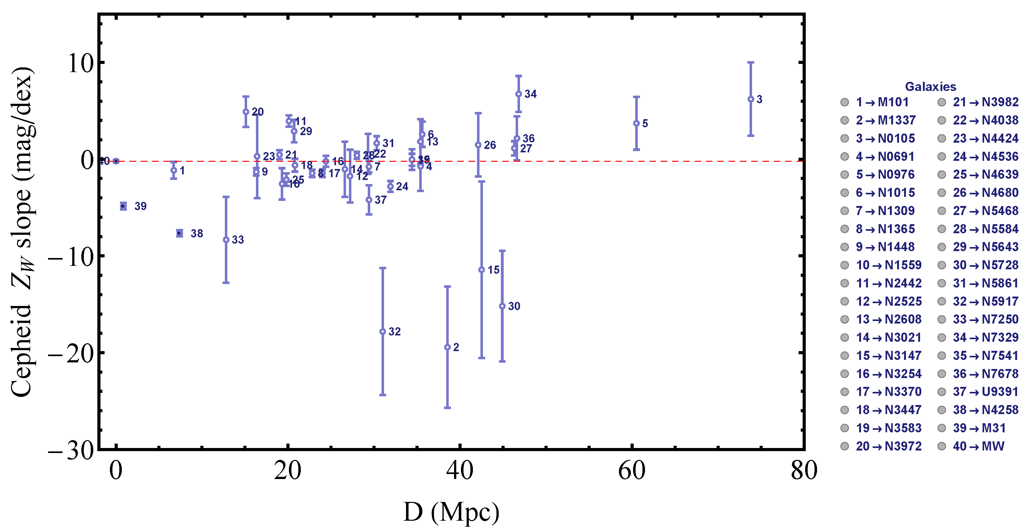
- It is evident by inspection of Figure 10 of R21 (see also Figure A4 below) that most of the better measured slopes have a smaller absolute slope than the corresponding slopes obtained from anchors+MW hosts. This makes it interesting to further test the homogeneity of these measurements and their consistency with the assumption of a global value of for both anchors and SnIa hosts.
- Most of the measurements that include outliers (red points of Figure 10 of R21) tend to amplify the above-mentioned effect, i.e., they have smaller absolute slopes than the slopes obtained from the anchors.
- The slope corresponding to the host N4424 is missing from Figure 10 of R21, while the host M1337 appears to show extreme behavior of the outliers.


| Galaxy | |||||||
|---|---|---|---|---|---|---|---|
| [Mpc] | [mag/dex] | [mag/dex] | [mag/dex] | [mag/dex] | [mag/dex] | [mag/dex] | |
| M101 | 6.71 | −2.99 | 0.14 | 0.18 | −1.14 | 0.86 | 3.2 |
| M1337 | 38.53 | −4. | 0.85 | 0.18 | −19.44 | 6.27 | 3.2 |
| N0691 | 35.4 | −2.64 | 0.57 | 0.18 | −0.73 | 2.54 | 3.2 |
| N1015 | 35.6 | −3.63 | 0.43 | 0.18 | 2.57 | 1.3 | 3.2 |
| N0105 | 73.8 | −5.13 | 2.13 | 0.18 | 6.21 | 3.8 | 3.2 |
| N1309 | 29.4 | −3.23 | 0.44 | 0.18 | −0.77 | 0.59 | 3.2 |
| N1365 | 22.8 | −2.9 | 0.37 | 0.18 | −1.45 | 0.39 | 3.2 |
| N1448 | 16.3 | −3.21 | 0.12 | 0.18 | −1.3 | 0.39 | 3.2 |
| N1559 | 19.3 | −3.27 | 0.18 | 0.18 | −2.55 | 1.62 | 3.2 |
| N2442 | 20.1 | −3.05 | 0.2 | 0.18 | 3.94 | 0.58 | 3.2 |
| N2525 | 27.2 | −3.2 | 0.37 | 0.18 | −1.75 | 2.74 | 3.2 |
| N2608 | 35.4 | −3.24 | 0.73 | 0.18 | 1.82 | 2.33 | 3.2 |
| N3021 | 26.6 | −3.3 | 0.89 | 0.18 | −1.03 | 2.85 | 3.2 |
| N3147 | 42.5 | −4.72 | 0.73 | 0.18 | −11.43 | 9.13 | 3.2 |
| N3254 | 24.4 | −3.05 | 0.31 | 0.18 | −0.22 | 0.57 | 3.2 |
| N3370 | 24 | −3.55 | 0.23 | 0.18 | −1.46 | 0.4 | 3.2 |
| N3447 | 20.8 | −3.48 | 0.13 | 0.18 | −0.62 | 0.66 | 3.2 |
| N3583 | 34.4 | −2.57 | 0.31 | 0.18 | −0.06 | 0.62 | 3.2 |
| N3972 | 15.1 | −3.58 | 0.32 | 0.18 | 4.9 | 1.58 | 3.2 |
| N3982 | 19 | −2.47 | 0.36 | 0.18 | 0.46 | 0.47 | 3.2 |
| N4038 | 29.3 | −2.63 | 0.47 | 0.18 | 0.54 | 2.07 | 3.2 |
| N4424 | 16.4 | 1.01 | 1.26 | 0.18 | 0.29 | 4.33 | 3.2 |
| N4536 | 31.9 | −3.25 | 0.19 | 0.18 | −2.82 | 0.56 | 3.2 |
| N4639 | 19.8 | −3.08 | 0.51 | 0.18 | −2.12 | 0.64 | 3.2 |
| N4680 | 42.1 | −3.12 | 1.22 | 0.18 | 1.48 | 3.27 | 3.2 |
| N5468 | 46.3 | −2.62 | 0.35 | 0.18 | 1.12 | 0.74 | 3.2 |
| N5584 | 28 | −3.26 | 0.16 | 0.18 | 0.4 | 0.36 | 3.2 |
| N5643 | 20.7 | −3.1 | 0.12 | 0.18 | 2.9 | 1.17 | 3.2 |
| N5728 | 44.9 | −5.09 | 1.34 | 0.18 | −15.19 | 5.71 | 3.2 |
| N5861 | 30.3 | −2.5 | 0.45 | 0.18 | 1.65 | 0.72 | 3.2 |
| N5917 | 31 | −4.54 | 1.17 | 0.18 | −17.82 | 6.56 | 3.2 |
| N7250 | 12.8 | −2.75 | 0.39 | 0.18 | −8.33 | 4.44 | 3.2 |
| N7329 | 46.8 | −3.04 | 0.76 | 0.18 | 6.74 | 1.86 | 3.2 |
| N7541 | 34.4 | −3.54 | 0.71 | 0.18 | −0.04 | 1.08 | 3.2 |
| N7678 | 46.6 | −2.73 | 1.03 | 0.18 | 2.16 | 2.27 | 3.2 |
| N0976 | 60.5 | −1.79 | 1.24 | 0.18 | 3.71 | 2.73 | 3.2 |
| U9391 | 29.4 | −3.33 | 0.43 | 0.18 | −4.2 | 1.51 | 3.2 |
| N4258 | 7.4 | −3.32 | 0.06 | 0.18 | −7.67 | 0.31 | 3.2 |
| M31 | 0.86 | −3.29 | 0.07 | 0.18 | −4.85 | 0.35 | 3.2 |
| LMC | 0.05 | −3.31 | 0.017 | 0.18 | − | − | 3.2 |
| SMC | 0.06 | −3.31 | 0.017 | 0.18 | − | − | 3.2 |
| MW | 0 | −3.26 | 0.05 | 0.18 | −0.2 | 0.12 | 3.2 |
Appendix D. Model Selection Criteria
| Level of empirical support for the model with the smaller | Evidence against the model with the larger | ||||||
| 0–2 | 4–7 | >10 | 0–2 | 2–6 | 6–10 | >10 | |
| Substantial | Strong | Very strong | Weak | Positive | Strong | Very strong | |
Appendix E
| Galaxy | Ranking | [P] | [O/H] | ||
|---|---|---|---|---|---|
| in Vector Y | [mag] | [mag] | [dex] | [dex] | |
| M1337 | 1 | 27.52 | 0.39 | 0.45 | −0.2 |
| M1337 | 2 | 28.05 | 0.47 | 0.65 | −0.19 |
| M1337 | 3 | 26.56 | 0.35 | 0.6 | −0.2 |
| M1337 | 4 | 26.97 | 0.27 | 0.78 | −0.2 |
| M1337 | 5 | 27.01 | 0.47 | 0.72 | −0.18 |
| M1337 | 6 | 26.29 | 0.5 | 0.9 | −0.17 |
| M1337 | 7 | 26.12 | 0.6 | 0.89 | −0.17 |
| M1337 | 8 | 26.94 | 0.45 | 0.75 | −0.17 |
| M1337 | 9 | 27.78 | 0.61 | 0.69 | −0.16 |
| M1337 | 10 | 26.17 | 0.55 | 0.7 | −0.14 |
| M1337 | 11 | 26.63 | 0.65 | 0.49 | −0.22 |
| M1337 | 12 | 27.4 | 0.39 | 0.85 | −0.19 |
| M1337 | 13 | 27.26 | 0.53 | 0.52 | −0.22 |
| M1337 | 14 | 27.34 | 0.34 | 0.85 | −0.17 |
| M1337 | 15 | 27 | 0.54 | 0.7 | −0.19 |
| N0691 | 1 | 26.59 | 0.57 | 0.4 | 0.09 |
| N0691 | 2 | 27.1 | 0.46 | 0.61 | 0.06 |
| N0691 | 3 | 26.79 | 0.47 | 0.71 | 0.04 |
| N0691 | 4 | 26.83 | 0.5 | 0.78 | 0.14 |
| N0691 | 5 | 26.23 | 0.44 | 0.51 | 0.05 |
| N0691 | 6 | 27.16 | 0.48 | 0.63 | 0.1 |
| N0691 | 7 | 26.89 | 0.46 | 0.7 | 0.03 |
| N0691 | 8 | 26.75 | 0.59 | 0.43 | 0.03 |
| N0691 | 9 | 27.11 | 0.28 | 0.88 | 0.04 |
| N0691 | 10 | 26.99 | 0.68 | 0.62 | 0.1 |
| N0691 | 11 | 27.6 | 0.35 | 0.81 | 0.07 |
| N0691 | 12 | 27.33 | 0.38 | 0.75 | 0.08 |
| N0691 | 13 | 26.6 | 0.53 | 0.54 | 0.14 |
| N0691 | 14 | 26.34 | 0.45 | 0.74 | 0.09 |
| N0691 | 15 | 26.91 | 0.3 | 0.96 | 0.11 |
| N0691 | 16 | 26.79 | 0.49 | 0.84 | 0.13 |
| N0691 | 17 | 27.08 | 0.48 | 0.63 | 0.1 |
| N0691 | 18 | 27.07 | 0.59 | 0.63 | 0.1 |
| N0691 | 19 | 26.69 | 0.63 | 0.53 | 0.07 |
| N0691 | 20 | 27.94 | 0.58 | 0.49 | 0.11 |
| N0691 | 21 | 26.15 | 0.62 | 0.48 | 0.12 |
| N0691 | 22 | 26.46 | 0.43 | 0.74 | 0.11 |
| N0691 | 23 | 27.16 | 0.6 | 0.42 | 0.14 |
| N0691 | 24 | 26.96 | 0.38 | 0.8 | 0.14 |
| N0691 | 25 | 26.59 | 0.44 | 0.65 | 0.04 |
| N0691 | 26 | 26.61 | 0.52 | 0.5 | 0.09 |
| N0691 | 27 | 26.21 | 0.6 | 0.62 | 0.11 |
| N0691 | 28 | 27.42 | 0.65 | 0.65 | 0.1 |
| … | … | … | … | … | … |
| 1 | At a distance [156], NGC4258 is the closest galaxy, beyond the Local Group with a geometric distance measurement. |
| 2 | A differential distance measurement of the SMC with respect to the LMC is used and thus LMC+SMC are considered in a unified manner in the released data. |
| 3 | 45 Cepheids in N1365 are mentioned in R21 but there are 46 in the fits files of the released dataset at Github repository: PantheonPlusSH0ES/DataRelease (accessed on 25 June 2022). |
| 4 | A total of 3130 Cepheids have been released in the data fits files but 3129 are mentioned in R21 (see Table 3). These data are also shown concisely in Table A3 of Appendix E and may be download in electronic form. |
| 5 | This parameter is not defined in R21 but is included in the data release fits files. We thank A. Riess for clarifying this point. |
| 6 | For Cepheids in the LMC/SMC anchor observed from the ground, the zeropoint parameter is added on the RHS, and thus Equation (6) becomes to allow for a different P-L zeropoint between ground and HST observations. |
| 7 | In the case of SMC, a differential distance with respect to LMC is used. |
| 8 | The , and matrices have been made publicly available as fits files by the SH0ES team at Github repository: PantheonPlusSH0ES/DataRelease (accessed on 25 June 2022). |
| 9 | The results for the parameters in are the same as the results obtained using the numerical minimization of (see the absolute matching of the results in the numerical analysis file “Baseline1 structure of system” in the A reanalysis of the SH0ES data for H0 GitHub repository (accessed on 23 August 2022)). |
| 10 | We use the standard notation which is important in the error propagation to . |
| 11 | 37 SnIa/Cepheid hosts and 3 pure Cepheid hosts of which 2 are anchors (N4258 and LMC) |
| 12 | As discussed in Appendix C, two slopes corresponding to the hosts N4038 and N1365 are slightly shifted in our analysis compared to R21 due a small disagreement in the best-fit slope and a typo of R21 in transferring the correct slope to Figure 10, while the slope corresponding to the host N4424 is missing in Figure 10 of R21. |
| 13 | The number of degrees of freedom is for and for . The smaller number of N for is due to the fact that metallicities were not provided for individual Cepheids in the LMC and SMS in R21, and thus, we evaluated a smaller number of slopes for . See also Table A1. The points shown in the plot Figure 1 include the two additional points corresponding to MW and SMC (which is degenerate with LMC). |
| 14 | Some hosts have more than one SnIa and more than one light curve and thus, averaging with proper uncertainties was implemented in these cases. |
| 15 | For more details see https://people.duke.edu/~hpgavin/SystemID/CourseNotes/linear-least-squres.pdf (accessed on 28 June 2022). |
References
- Riess, A.G.; Yuan, W.; Macri, L.M.; Scolnic, D.; Brout, D.; Casertano, S.; Jones, D.O.; Murakami, Y.; Anand, G.S.; Breuval, L.; et al. A Comprehensive Measurement of the Local Value of the Hubble Constant with 1 km s-1 Mpc-1 Uncertainty from the Hubble Space Telescope and the SH0ES Team. Astrophys. J. Lett. 2022, 934, L7. [Google Scholar] [CrossRef]
- Freedman, W.L. Measurements of the Hubble Constant: Tensions in Perspective. arXiv 2021, arXiv:2106.15656. [Google Scholar] [CrossRef]
- Gómez-Valent, A.; Amendola, L. H0 from cosmic chronometers and Type Ia supernovae, with Gaussian Processes and the novel Weighted Polynomial Regression method. J. Cosmol. Astropart. Phys. 2018, 04, 051. [Google Scholar] [CrossRef]
- Pesce, D.; Braatz, J.A.; Reid, M.J.; Riess, A.G.; Scolnic, D.; Condon, J.J.; Gao, F.; Henkel, C.; Impellizzeri, C.M.V.; Kuo, C.Y.; et al. The Megamaser Cosmology Project. XIII. Combined Hubble constant constraints. Astrophys. J. Lett. 2020, 891, L1. [Google Scholar] [CrossRef]
- Freedman, W.L.; Madore, B.F.; Hoyt, T.; Jang, I.S.; Beaton, R.; Lee, M.G.; Monson, A.; Neeley, J.; Rich, J. Calibration of the Tip of the Red Giant Branch (TRGB). arXiv 2020, arXiv:2002.01550. [Google Scholar]
- Wong, K.C.; Suyu, S.H.; Chen, G.C.-F.; E Rusu, C.; Millon, M.; Sluse, D.; Bonvin, V.; Fassnacht, C.D.; Taubenberger, S.; Auger, M.W.; et al. H0LiCOW – XIII. A 2.4 per cent measurement of H0 from lensed quasars: 5.3σ tension between early- and late-Universe probes. Mon. Not. Roy. Astron. Soc. 2020, 498, 1420–1439. [Google Scholar] [CrossRef]
- Chen, G.C.F.; Fassnacht, C.; Suyu, S.H.; E Rusu, C.; Chan, J.H.H.; Wong, K.C.; Auger, M.W.; Hilbert, S.; Bonvin, V.; Birrer, S.; et al. A SHARP view of H0LiCOW: H0 from three time-delay gravitational lens systems with adaptive optics imaging. Mon. Not. Roy. Astron. Soc. 2019, 490, 1743–1773. [Google Scholar] [CrossRef]
- Birrer, S.; Shajib, A.J.; Galan, A.; Millon, M.; Treu, T.; Agnello, A.; Auger, M.; Chen, G.C.-F.; Christensen, L.; Van de Vyvere, L.; et al. TDCOSMO - IV. Hierarchical time-delay cosmography – joint inference of the Hubble constant and galaxy density profiles. Astron. Astrophys. 2020, 643, A165. [Google Scholar] [CrossRef]
- Birrer, S.; Treu, T.; E Rusu, C.; Bonvin, V.; Fassnacht, C.; Chan, J.H.H.; Agnello, A.; Shajib, A.J.; Chen, G.C.-F.; Auger, M.; et al. Cosmographic analysis of the doubly imaged quasar SDSS 1206+4332 and a new measurement of the Hubble constant. Mon. Not. Roy. Astron. Soc. 2019, 484, 4726. [Google Scholar] [CrossRef]
- Fishbach, M.; Gray, R.; Hernandez, I.M.; Qi, H.; Sur, A.; Acernese, F.; Aiello, L.; Allocca, A.; Aloy, M.A.; Amato, A.; et al. A Standard Siren Measurement of the Hubble Constant from GW170817 without the Electromagnetic Counterpart. Astrophys. J. Lett. 2019, 871, L13. [Google Scholar] [CrossRef]
- Hotokezaka, K.; Nakar, E.; Gottlieb, O.; Nissanke, S.; Masuda, K.; Hallinan, G.; Mooley, K.P.; Deller, A.T. A Hubble constant measurement from superluminal motion of the jet in GW170817. Nature Astron. 2019, 3, 940–944. [Google Scholar] [CrossRef] [Green Version]
- Abbott, B.P.; Shajib, A.J.; Galan, A.; Millon, M.; Treu, T.; Agnello, A.; Auger, M.; Chen, G.C.-F.; Christensen, L.; Collett, T.; et al. A gravitational-wave standard siren measurement of the Hubble constant. Nature 2017, 551, 85–88. [Google Scholar] [CrossRef]
- Palmese, A.; Devicente, J.; Pereira, M.E.S.; Annis, J.; Hartley, W.; Herner, K.; Soares-Santos, M.; Crocce, M.; Huterer, D.; Magaña Hernandez, I.; et al. A statistical standard siren measurement of the Hubble constant from the LIGO/Virgo gravitational wave compact object merger GW190814 and Dark Energy Survey galaxies. Astrophys. J. Lett. 2020, 900, L33. [Google Scholar] [CrossRef]
- Soares-Santos, M.; Palmese, A.; Hartley, W.; Annis, J.; Garcia-Bellido, J.; Lahav, O.; Doctor, Z.; Fishbach, M.; Holz, D.E.; Lin, H.; et al. First Measurement of the Hubble Constant from a Dark Standard Siren using the Dark Energy Survey Galaxies and the LIGO/Virgo Binary–Black-hole Merger GW170814. Astrophys. J. Lett. 2019, 876, L7. [Google Scholar] [CrossRef]
- Cao, S.; Dainotti, M.; Ratra, B. Standardizing Platinum Dainotti-correlated gamma-ray bursts, and using them with standardized Amati-correlated gamma-ray bursts to constrain cosmological model parameters. Mon. Not. Roy. Astron. Soc. 2022, 512, 439–454. [Google Scholar] [CrossRef]
- Cao, S.; Dainotti, M.; Ratra, B. Gamma-ray burst data strongly favor the three-parameter fundamental plane (Dainotti) correlation relation over the two-parameter one. Mon. Not. R. Astron. Soc. 2022, 516, 1386–1405. [Google Scholar] [CrossRef]
- Dainotti, M.G.; Sarracino, G.; Capozziello, S. Gamma-Ray Bursts, Supernovae Ia and Baryon Acoustic Oscillations: A binned cosmological analysis. Publ. Astron. Soc. Jpn. 2022, 74, 1095–1113. [Google Scholar] [CrossRef]
- Dainotti, M.G.; Nielson, V.; Sarracino, G.; Rinaldi, E.; Nagataki, S.; Capozziello, S.; Gnedin, O.Y.; Bargiacchi, G. Optical and X-ray GRB Fundamental Planes as cosmological distance indicators. Mon. Not. Roy. Astron. Soc. 2022, 514, 1828–1856. [Google Scholar] [CrossRef]
- Dainotti, M.G.; Cardone, V.F.; Piedipalumbo, E.; Capozziello, S. Slope evolution of GRB correlations and cosmology. Mon. Not. Roy. Astron. Soc. 2013, 436, 82. [Google Scholar] [CrossRef]
- Risaliti, G.; Lusso, E. Cosmological constraints from the Hubble diagram of quasars at high redshifts. Nat. Astron. 2019, 3, 272–277. [Google Scholar] [CrossRef]
- de Jaeger, T.; Galbany, L.; Riess, A.G.; Stahl, B.E.; Shappee, B.J.; Filippenko, A.V.; Zheng, W. A 5% measurement of the Hubble constant from Type II supernovae. Mon. Not. R. Astron. Soc. 2020, 514, 4620–4628. [Google Scholar] [CrossRef]
- de Jaeger, T.; Stahl, B.; Zheng, W.; Filippenko, A.; Riess, A.; Galbany, L. A measurement of the Hubble constant from Type II supernovae. Mon. Not. R. Astron. Soc. 2020, 496, 3402–3411. [Google Scholar] [CrossRef]
- Domínguez, A.; Wojtak, R.; Finke, J.; Ajello, M.; Helgason, K.; Prada, F.; Desai, A.; Paliya, V.; Marcotulli, L.; Hartmann, D. A new measurement of the Hubble constant and matter content of the Universe using extragalactic background light γ-ray attenuation. Astrophys. J. 2019, 885, 137. [Google Scholar] [CrossRef]
- Di Valentino, E.; Mena, O.; Pan, S.; Visinelli, L.; Yang, W.; Melchiorri, A.; Mota, D.F.; Riess, A.G.; Silk, J. In the realm of the Hubble tension—a review of solutions. Class. Quant. Grav. 2021, 38, 153001. [Google Scholar] [CrossRef]
- Perivolaropoulos, L.; Skara, F. Challenges for ΛCDM: An update. New Astron. Rev. 2022, 95, 101659. [Google Scholar] [CrossRef]
- Aghanim, N.; Akrami, Y.; Ashdown, M.; Aumont, J.; Baccigalupi, C.; Ballardini, M.; Banday, A.I.; Barreiro, R.B.; Bartolo, N.; Basak, S.; et al. Planck 2018 results. VI. Cosmological parameters. Astron. Astrophys. 2020, 641, A6, Erratum Astron. Astrophys. 2021, 652, C4. [Google Scholar] [CrossRef]
- Abdalla, E.; Abellán, G.F.; Aboubrahim, A.; Agnello, A.; Akarsu, O.; Akrami, Y.; Alestas, G.; Aloni, D.; Amendola, L.; Anchordoqui, L.A.; et al. Cosmology intertwined: A review of the particle physics, astrophysics, and cosmology associated with the cosmological tensions and anomalies. JHEAp 2022, 34, 49–211. [Google Scholar] [CrossRef]
- Shah, P.; Lemos, P.; Lahav, O. A buyer’s guide to the Hubble constant. Astron. Astrophys. Rev. 2021, 29, 9. [Google Scholar] [CrossRef]
- Knox, L.; Millea, M. The Hubble Hunter’s Guide. arXiv 2019, arXiv:1908.03663. [Google Scholar]
- Vagnozzi, S. New physics in light of the H0 tension: An alternative view. Phys. Rev. D 2020, 102, 023518. [Google Scholar] [CrossRef]
- Ishak, M. Testing General Relativity in Cosmology. Living Rev. Rel. 2019, 22, 1. [Google Scholar] [CrossRef] [PubMed]
- Mörtsell, E.; Dhawan, S. Does the Hubble constant tension call for new physics? JCAP 2018, 1809, 025. [Google Scholar] [CrossRef] [Green Version]
- Huterer, D.; Shafer, D.L. Dark energy two decades after: Observables, probes, consistency tests. Rept. Prog. Phys. 2018, 81, 016901. [Google Scholar] [CrossRef]
- Bernal, J.L.; Verde, L.; Riess, A.G. The trouble with H0. JCAP 2016, 1610, 019. [Google Scholar] [CrossRef]
- Alam, S.; Aubert, M.; Avila, S.; Balland, C.; Bautista, J.E.; Bershady, M.A.; Bizyaev, D.; Blanton, M.R.; Bolton, A.S.; Bovy, J.; et al. Completed SDSS-IV extended Baryon Oscillation Spectroscopic Survey: Cosmological implications from two decades of spectroscopic surveys at the Apache Point Observatory. Phys. Rev. D 2021, 103, 083533. [Google Scholar] [CrossRef]
- Verde, L.; Treu, T.; Riess, A.G. Tensions between the Early and the Late Universe. Nature Astron. 2019, 3, 891. [Google Scholar] [CrossRef]
- Schöneberg, N.; Franco Abellán, G.; Pérez Sánchez, A.; Witte, S.J.; Poulin, V.; Lesgourgues, J. The H0 Olympics: A fair ranking of proposed models. arXiv 2021, arXiv:2107.10291. [Google Scholar] [CrossRef]
- Krishnan, C.; Colgáin, E.O.; Ruchika; Sen, A.A.; Sheikh-Jabbari, M.M.; Yang, T. Is there an early Universe solution to Hubble tension? Phys. Rev. D 2020, 102, 103525. [Google Scholar] [CrossRef]
- Jedamzik, K.; Pogosian, L.; Zhao, G.B. Why reducing the cosmic sound horizon can not fully resolve the Hubble tension. arXiv 2020, arXiv:2010.04158. [Google Scholar]
- Poulin, V.; Smith, T.L.; Karwal, T.; Kamionkowski, M. Early Dark Energy Can Resolve The Hubble Tension. Phys. Rev. Lett. 2019, 122, 221301. [Google Scholar] [CrossRef]
- Niedermann, F.; Sloth, M.S. New early dark energy. Phys. Rev. D 2021, 103, L041303. [Google Scholar] [CrossRef]
- Smith, T.L.; Lucca, M.; Poulin, V.; Abellan, G.F.; Balkenhol, L.; Benabed, K.; Galli, S.; Murgia, R. Hints of Early Dark Energy in Planck, SPT, and ACT data: New physics or systematics? arXiv 2022, arXiv:2202.09379. [Google Scholar] [CrossRef]
- Smith, T.L.; Poulin, V.; Bernal, J.L.; Boddy, K.K.; Kamionkowski, M.; Murgia, R. Early dark energy is not excluded by current large-scale structure data. arXiv 2020, arXiv:2009.10740. [Google Scholar] [CrossRef]
- Chudaykin, A.; Gorbunov, D.; Nedelko, N. Combined analysis of Planck and SPTPol data favors the early dark energy models. J. Cosmol. Astropart. Phys. 2020, 08, 013. [Google Scholar] [CrossRef]
- Fondi, E.; Melchiorri, A.; Pagano, L. No evidence for EDE from Planck data in extended scenarios. Astrophys. J. Lett. 2022, 931, L18. [Google Scholar]
- Sabla, V.I.; Caldwell, R.R. The Microphysics of Early Dark Energy. arXiv 2022, arXiv:2202.08291. [Google Scholar] [CrossRef]
- Herold, L.; Ferreira, E.G.M.; Komatsu, E. New Constraint on Early Dark Energy from Planck and BOSS Data Using the Profile Likelihood. Astrophys. J. Lett. 2022, 929, L16. [Google Scholar] [CrossRef]
- McDonough, E.; Lin, M.X.; Hill, J.C.; Hu, W.; Zhou, S. Early dark sector, the Hubble tension, and the swampland. Phys. Rev. D 2022, 106, 043525. [Google Scholar] [CrossRef]
- Hill, J.C.; McDonough, E.; Toomey, M.W.; Alexander, S. Early Dark Energy Does Not Restore Cosmological Concordance. arXiv 2020, arXiv:2003.07355. [Google Scholar] [CrossRef]
- Sakstein, J.; Trodden, M. Early Dark Energy from Massive Neutrinos as a Natural Resolution of the Hubble Tension. Phys. Rev. Lett. 2020, 124, 161301. [Google Scholar] [CrossRef]
- Niedermann, F.; Sloth, M.S. New Early Dark Energy is compatible with current LSS data. arXiv 2020, arXiv:2009.00006. [Google Scholar] [CrossRef]
- Rezazadeh, K.; Ashoorioon, A.; Grin, D. Cascading Dark Energy. arXiv 2022, arXiv:2208.07631. [Google Scholar]
- Green, D.; Amin, M.A.; Meyers, J.; Wallisch, B.; Abazajian, K.N.; Abidi, M.; Adshead, P.; Ahmed, Z.; Ansarinejad, B.; Armstrong, R.; et al. Messengers from the Early Universe: Cosmic Neutrinos and Other Light Relics. Bull. Am. Astron. Soc. 2019, 51, 159. [Google Scholar]
- Schöneberg, N.; Franco Abellán, G. A step in the right direction? Analyzing the Wess Zumino Dark Radiation solution to the Hubble tension. arXiv 2022, arXiv:2206.11276. [Google Scholar]
- Seto, O.; Toda, Y. Comparing early dark energy and extra radiation solutions to the Hubble tension with BBN. arXiv 2021, arXiv:2101.03740. [Google Scholar] [CrossRef]
- Carrillo González, M.; Liang, Q.; Sakstein, J.; Trodden, M. Neutrino-Assisted Early Dark Energy: Theory and Cosmology. arXiv 2020, arXiv:2011.09895. [Google Scholar] [CrossRef]
- Braglia, M.; Ballardini, M.; Finelli, F.; Koyama, K. Early modified gravity in light of the H0 tension and LSS data. Phys. Rev. D 2021, 103, 043528. [Google Scholar] [CrossRef]
- Abadi, T.; Kovetz, E.D. Can conformally coupled modified gravity solve the Hubble tension? Phys. Rev. D 2021, 103, 023530. [Google Scholar] [CrossRef]
- Renk, J.; Zumalacárregui, M.; Montanari, F.; Barreira, A. Galileon gravity in light of ISW, CMB, BAO and H0 data. J. Cosmol. Astropart. Phys. 2017, 1710, 020. [Google Scholar] [CrossRef]
- Nojiri, S.; Odintsov, S.D.; Oikonomou, V.K. Integral F(R) gravity and saddle point condition as a remedy for the H0-tension. Nucl. Phys. B 2022, 980, 115850. [Google Scholar] [CrossRef]
- Lin, M.X.; Raveri, M.; Hu, W. Phenomenology of Modified Gravity at Recombination. Phys. Rev. 2019, D99, 043514. [Google Scholar] [CrossRef]
- Saridakis, E.N.; Lazkoz, R.; Salzano, V.; Moniz, P.V.; Capozziello, S.; Jiménez, J.B.; De Laurentis, M.; Olmo, G.J. Modified Gravity and Cosmology: An Update by the CANTATA Network. arXiv 2021, arXiv:2105.12582. [Google Scholar]
- Benisty, D. Quantifying the S8 tension with the Redshift Space Distortion data set. Phys. Dark Univ. 2021, 31, 100766. [Google Scholar] [CrossRef]
- Heymans, C.; Tröster, T.; Asgari, M.; Blake, C.; Hildebrandt, H.; Joachimi, B.; Kuijken, K.; Lin, C.-A.; Sánchez, A.G.; Busch, J.L.V.D.; et al. KiDS-1000 Cosmology: Multi-probe weak gravitational lensing and spectroscopic galaxy clustering constraints. Astron. Astrophys. 2021, 646, A140. [Google Scholar] [CrossRef]
- Kazantzidis, L.; Perivolaropoulos, L. Evolution of the fσ8 tension with the Planck15/ΛCDM determination and implications for modified gravity theories. Phys. Rev. D 2018, 97, 103503. [Google Scholar] [CrossRef]
- Joudaki, S.; Blake, C.; Johnson, A.; Amon, A.; Asgari, M.; Choi, A.; Erben, T.; Glazebrook, K.; Harnois-Déraps, J.; Heymans, C.; et al. KiDS-450 + 2dFLenS: Cosmological parameter constraints from weak gravitational lensing tomography and overlapping redshift-space galaxy clustering. Mon. Not. Roy. Astron. Soc. 2018, 474, 4894–4924. [Google Scholar] [CrossRef]
- Kazantzidis, L.; Perivolaropoulos, L. σ8 Tension.Is Gravity Getting Weaker at Low z? Observational Evidence and Theoretical Implications. In Modified Gravity and Cosmology; Springer: Cham, Switzerland, 2019; pp. 507–537. [Google Scholar] [CrossRef]
- Skara, F.; Perivolaropoulos, L. Tension of the EG statistic and redshift space distortion data with the Planck - ΛCDM model and implications for weakening gravity. Phys. Rev. D 2020, 101, 063521. [Google Scholar] [CrossRef] [Green Version]
- Avila, F.; Bernui, A.; Bonilla, A.; Nunes, R.C. Inferring S8(z) and γ(z) with cosmic growth rate measurements using machine learning. Eur. Phys. J. C 2022, 82, 594. [Google Scholar] [CrossRef]
- Köhlinger, F.; Viola, M.; Joachimi, B.; Hoekstra, H.; Van Uitert, E.; Hildebrandt, H.; Choi, A.; Erben, T.; Heymans, C.; Joudaki, S.; et al. KiDS-450: The tomographic weak lensing power spectrum and constraints on cosmological parameters. Mon. Not. Roy. Astron. Soc. 2017, 471, 4412–4435. [Google Scholar] [CrossRef]
- Nunes, R.C.; Vagnozzi, S. Arbitrating the S8 discrepancy with growth rate measurements from redshift-space distortions. Mon. Not. Roy. Astron. Soc. 2021, 505, 5427–5437. [Google Scholar] [CrossRef]
- Clark, S.J.; Vattis, K.; Fan, J.; Koushiappas, S.M. The H0 and S8 tensions necessitate early and late time changes to ΛCDM. arXiv 2021, arXiv:2110.09562. [Google Scholar]
- Ivanov, M.M.; McDonough, E.; Hill, J.C.; Simonović, M.; Toomey, M.W.; Alexander, S.; Zaldarriaga, M. Constraining Early Dark Energy with Large-Scale Structure. Phys. Rev. D 2020, 102, 103502. [Google Scholar] [CrossRef]
- Hill, J.C.; Calabrese, E.; Aiola, S.; Battaglia, N.; Bolliet, B.; Choi, S.K.; Devlin, M.J.; Duivenvoorden, A.J.; Dunkley, J.; Ferraro, S.; et al. Atacama Cosmology Telescope: Constraints on prerecombination early dark energy. Phys. Rev. D 2022, 105, 123536. [Google Scholar] [CrossRef]
- Vagnozzi, S. Consistency tests of ΛCDM from the early integrated Sachs-Wolfe effect: Implications for early-time new physics and the Hubble tension. Phys. Rev. D 2021, 104, 063524. [Google Scholar] [CrossRef]
- Philcox, O.H.E.; Farren, G.S.; Sherwin, B.D.; Baxter, E.J.; Brout, D.J. Determining the Hubble Constant without the Sound Horizon: A 3.6% Constraint on H0 from Galaxy Surveys, CMB Lensing and Supernovae. arXiv 2022, arXiv:2204.02984. [Google Scholar] [CrossRef]
- Chudaykin, A.; Gorbunov, D.; Nedelko, N. Exploring an early dark energy solution to the Hubble tension with Planck and SPTPol data. Phys. Rev. D 2021, 103, 043529. [Google Scholar] [CrossRef]
- Reeves, A.; Herold, L.; Vagnozzi, S.; Sherwin, B.D.; Ferreira, E.G.M. Restoring cosmological concordance with early dark energy and massive neutrinos? arXiv 2022, arXiv:2207.01501. [Google Scholar]
- Solà Peracaula, J.; Gómez-Valent, A.; de Cruz Pérez, J.; Moreno-Pulido, C. Brans–Dicke cosmology with a Λ-term: A possible solution to ΛCDM tensions. Class. Quant. Grav. 2020, 37, 245003. [Google Scholar] [CrossRef]
- Braglia, M.; Ballardini, M.; Emond, W.T.; Finelli, F.; Gumrukcuoglu, A.E.; Koyama, K.; Paoletti, D. Larger value for H0 by an evolving gravitational constant. Phys. Rev. D 2020, 102, 023529. [Google Scholar] [CrossRef]
- Pogosian, L.; Raveri, M.; Koyama, K.; Martinelli, M.; Silvestri, A.; Zhao, G.B. Imprints of cosmological tensions in reconstructed gravity. arXiv 2021, arXiv:2107.12992. [Google Scholar]
- Bahamonde, S.; Dialektopoulos, K.F.; Escamilla-Rivera, C.; Farrugia, G.; Gakis, V.; Hendry, M.; Hohmann, M.; Said, J.L.; Mifsud, J.; Di Valentino, E. Teleparallel Gravity: From Theory to Cosmology. arXiv 2021, arXiv:2106.13793. [Google Scholar]
- Di Valentino, E.; Mukherjee, A.; Sen, A.A. Dark Energy with Phantom Crossing and the H0 Tension. Entropy 2021, 23, 404. [Google Scholar] [CrossRef] [PubMed]
- Alestas, G.; Kazantzidis, L.; Perivolaropoulos, L. H0 Tension, Phantom Dark Energy and Cosmological Parameter Degeneracies. Phys. Rev. D 2020, 101, 123516. [Google Scholar] [CrossRef]
- Di Valentino, E.; Melchiorri, A.; Mena, O.; Vagnozzi, S. Nonminimal dark sector physics and cosmological tensions. Phys. Rev. D 2020, 101, 063502. [Google Scholar] [CrossRef]
- Pan, S.; Yang, W.; Di Valentino, E.; Shafieloo, A.; Chakraborty, S. Reconciling H0 tension in a six parameter space? J. Cosmol. Astropart. Phys. 2020, 06, 062. [Google Scholar] [CrossRef]
- Li, X.; Shafieloo, A. A Simple Phenomenological Emergent Dark Energy Model can Resolve the Hubble Tension. Astrophys. J. Lett. 2019, 883, L3. [Google Scholar] [CrossRef]
- Zhao, G.B.; Raveri, M.; Pogosian, L.; Wang, Y.; Crittenden, R.G.; Handley, W.; Percival, W.J.; Beutler, F.; Brinkmann, J.; Chuang, C.-H.; et al. Dynamical dark energy in light of the latest observations. Nature Astron. 2017, 1, 627–632. [Google Scholar] [CrossRef]
- Keeley, R.E.; Joudaki, S.; Kaplinghat, M.; Kirkby, D. Implications of a transition in the dark energy equation of state for the H0 and σ8 tensions. J. Cosmol. Astropart. Phys. 2019, 12, 035. [Google Scholar] [CrossRef]
- Sola Peracaula, J.; Gomez-Valent, A.; de Cruz Pérez, J. Signs of Dynamical Dark Energy in Current Observations. Phys. Dark Univ. 2019, 25, 100311. [Google Scholar] [CrossRef]
- Yang, W.; Pan, S.; Di Valentino, E.; Saridakis, E.N.; Chakraborty, S. Observational constraints on one-parameter dynamical dark-energy parametrizations and the H0 tension. Phys. Rev. 2019, D99, 043543. [Google Scholar] [CrossRef]
- Krishnan, C.; Colgáin, E.O.; Sheikh-Jabbari, M.M.; Yang, T. Running Hubble Tension and a H0 Diagnostic. Phys. Rev. D 2021, 103, 103509. [Google Scholar] [CrossRef]
- Dainotti, M.G.; De Simone, B.; Schiavone, T.; Montani, G.; Rinaldi, E.; Lambiase, G. On the Hubble constant tension in the SNe Ia Pantheon sample. Astrophys. J. 2021, 912, 150. [Google Scholar] [CrossRef]
- Colgáin, E.O.; Sheikh-Jabbari, M.M.; Solomon, R.; Bargiacchi, G.; Capozziello, S.; Dainotti, M.G.; Stojkovic, D. Revealing intrinsic flat ΛCDM biases with standardizable candles. Phys. Rev. D 2022, 106, L041301. [Google Scholar] [CrossRef]
- Colgáin, E.O.; Sheikh-Jabbari, M.M.; Solomon, R.; Dainotti, M.G.; Stojkovic, D. Putting Flat ΛCDM In The (Redshift) Bin. arXiv 2022, arXiv:2206.11447. [Google Scholar]
- Zhou, Z.; Liu, G.; Xu, L. Can late dark energy restore the Cosmic concordance? arXiv 2021, arXiv:2105.04258. [Google Scholar]
- Di Valentino, E.; Melchiorri, A.; Mena, O.; Vagnozzi, S. Interacting dark energy in the early 2020s: A promising solution to the H0 and cosmic shear tensions. Phys. Dark Univ. 2020, 30, 100666. [Google Scholar] [CrossRef]
- Yang, W.; Pan, S.; Di Valentino, E.; Nunes, R.C.; Vagnozzi, S.; Mota, D.F. Tale of stable interacting dark energy, observational signatures, and the H0 tension. J. Cosmol. Astropart. Phys. 2018, 1809, 019. [Google Scholar] [CrossRef]
- Vattis, K.; Koushiappas, S.M.; Loeb, A. Dark matter decaying in the late Universe can relieve the H0 tension. Phys. Rev. 2019, D99, 121302. [Google Scholar] [CrossRef]
- Yang, W.; Mukherjee, A.; Di Valentino, E.; Pan, S. Interacting dark energy with time varying equation of state and the H0 tension. Phys. Rev. 2018, D98, 123527. [Google Scholar] [CrossRef]
- Ghosh, S.; Khatri, R.; Roy, T.S. Can dark neutrino interactions phase out the Hubble tension? Phys. Rev. D 2020, 102, 123544. [Google Scholar] [CrossRef]
- Brieden, S.; Gil-Marín, H.; Verde, L. Model-agnostic interpretation of 10 billion years of cosmic evolution traced by BOSS and eBOSS data. J. Cosmol. Astropart. Phys. 2022, 08, 024. [Google Scholar] [CrossRef]
- Alestas, G.; Perivolaropoulos, L. Late time approaches to the Hubble tension deforming H(z), worsen the growth tension. Mon. Not. Roy. Astron. Soc. 2021, 504, 3956. [Google Scholar] [CrossRef]
- Keeley, R.E.; Shafieloo, A. Ruling Out New Physics at Low Redshift as a solution to the H0 Tension. arXiv 2022, arXiv:2206.08440. [Google Scholar]
- Clark, S.J.; Vattis, K.; Koushiappas, S.M. CMB constraints on late-universe decaying dark matter as a solution to the H0 tension. arXiv 2020, arXiv:2006.03678. [Google Scholar]
- Chen, A.; Huterer, D.; Lee, S.; Ferté, A.; Weaverdyck, N.; Alves, O.; Leonard, C.D.; MacCrann, N.; Raveri, M.; Porredon, A.; et al. Constraints on dark matter to dark radiation conversion in the late universe with DES-Y1 and external data. Phys. Rev. D 2021, 103, 123528. [Google Scholar] [CrossRef]
- Anchordoqui, L.A.; Barger, V.; Marfatia, D.; Soriano, J.F. Decay of multiple dark matter particles to dark radiation in different epochs does not alleviate the Hubble tension. Phys. Rev. D 2022, 105, 103512. [Google Scholar] [CrossRef]
- Mau, S.; Nadler, E.O.; Wechsler, R.H.; Drlica-Wagner, A.; Bechtol, K.; Green, G.; Huterer, D.; Li, T.S.; Mao, Y.-Y.; Martínez-Vázquez, C.E.; et al. Milky Way Satellite Census. IV. Constraints on Decaying Dark Matter from Observations of Milky Way Satellite Galaxies. Astrophys. J. 2022, 932, 128. [Google Scholar] [CrossRef]
- Cai, R.G.; Guo, Z.K.; Wang, S.J.; Yu, W.W.; Zhou, Y. No-go guide for the Hubble tension: Matter perturbations. arXiv 2020, arXiv:2202.12214. [Google Scholar]
- Heisenberg, L.; Villarrubia-Rojo, H.; Zosso, J. Can late-time extensions solve the H0 and σ8 tensions? Phys. Rev. D 2022, 106, 043503. [Google Scholar] [CrossRef]
- Vagnozzi, S.; Pacucci, F.; Loeb, A. Implications for the Hubble tension from the ages of the oldest astrophysical objects. JHEAp 2022, 36, 27–35. [Google Scholar] [CrossRef]
- Davari, Z.; Khosravi, N. Can decaying dark matter scenarios alleviate both H0 and σ8 tensions? arXiv 2020, arXiv:2203.09439. [Google Scholar] [CrossRef]
- Mortsell, E.; Goobar, A.; Johansson, J.; Dhawan, S. The Hubble Tension Bites the Dust: Sensitivity of the Hubble Constant Determination to Cepheid Color Calibration. arXiv 2021, arXiv:2105.11461. [Google Scholar]
- Efstathiou, G. H0 Revisited. Mon. Not. Roy. Astron. Soc. 2014, 440, 1138–1152. [Google Scholar] [CrossRef]
- Efstathiou, G. A Lockdown Perspective on the Hubble Tension (with comments from the SH0ES team). arXiv 2020, arXiv:2007.10716. [Google Scholar]
- Efstathiou, G. To H0 or not to H0? arXiv 2021, arXiv:2103.08723. [Google Scholar] [CrossRef]
- Wojtak, R.; Hjorth, J. Intrinsic tension in the supernova sector of the local Hubble constant measurement and its implications. arXiv 2022, arXiv:2206.08160. [Google Scholar] [CrossRef]
- Benisty, D.; Mifsud, J.; Said, J.L.; Staicova, D. On the Robustness of the Constancy of the Supernova Absolute Magnitude: Non-parametric Reconstruction & Bayesian approaches. arXiv 2022, arXiv:2202.04677. [Google Scholar]
- Martinelli, M.; Tutusaus, I. CMB tensions with low-redshift H0 and S8 measurements: Impact of a redshift-dependent type-Ia supernovae intrinsic luminosity. Symmetry 2019, 11, 986. [Google Scholar] [CrossRef]
- Tinsley, B.M. Evolution of the Stars and Gas in Galaxies. Astroph. J. 1968, 151, 547. [Google Scholar] [CrossRef]
- Kang, Y.; Lee, Y.W.; Kim, Y.L.; Chung, C.; Ree, C.H. Early-type Host Galaxies of Type Ia Supernovae. II. Evidence for Luminosity Evolution in Supernova Cosmology. Astrophys. J. 2020, 889, 8. [Google Scholar] [CrossRef]
- Rose, B.M.; Garnavich, P.M.; Berg, M.A. Think Global, Act Local: The Influence of Environment Age and Host Mass on Type Ia Supernova Light Curves. Astrophys. J. 2019, 874, 32. [Google Scholar] [CrossRef]
- Jones, D.O.; Riess, A.G.; Scolnic, D.M.; Pan, Y.-C.; Johnson, E.; Coulter, D.A.; Dettman, K.; Foley, M.; Foley, R.J.; Huber, M.E.; et al. Should Type Ia Supernova Distances be Corrected for their Local Environments? Astrophys. J. 2018, 867, 108. [Google Scholar] [CrossRef]
- Rigault, M.; Brinnel, V.; Aldering, G.; Antilogus, P.; Aragon, C.; Bailey, S.; Baltay, C.; Barbary, K.; Bongard, S.; Boone, K.; et al. Strong Dependence of Type Ia Supernova Standardization on the Local Specific Star Formation Rate. Astron. Astrophys. 2020, 644, A176. [Google Scholar] [CrossRef]
- Kim, Y.L.; Smith, M.; Sullivan, M.; Lee, Y.W. Environmental Dependence of Type Ia Supernova Luminosities from a Sample without a Local-Global Difference in Host Star Formation. Astroph. J. 2018, 854, 24. [Google Scholar] [CrossRef]
- Colgáin, E.O. A hint of matter underdensity at low z? J. Cosmol. Astropart. Phys. 2019, 09, 006. [Google Scholar] [CrossRef]
- Kazantzidis, L.; Perivolaropoulos, L. Hints of a Local Matter Underdensity or Modified Gravity in the Low z Pantheon data. Phys. Rev. D 2020, 102, 023520. [Google Scholar] [CrossRef]
- Sapone, D.; Nesseris, S.; Bengaly, C.A.P. Is there any measurable redshift dependence on the SN Ia absolute magnitude? Phys. Dark Univ. 2021, 32, 100814. [Google Scholar] [CrossRef]
- Koo, H.; Shafieloo, A.; Keeley, R.E.; L’Huillier, B. Model-independent Constraints on Type Ia Supernova Light-curve Hyperparameters and Reconstructions of the Expansion History of the Universe. Astrophys. J. 2020, 899, 9. [Google Scholar] [CrossRef]
- Kazantzidis, L.; Koo, H.; Nesseris, S.; Perivolaropoulos, L.; Shafieloo, A. Hints for possible low redshift oscillation around the best-fitting ΛCDM model in the expansion history of the Universe. Mon. Not. Roy. Astron. Soc. 2021, 501, 3421–3426. [Google Scholar] [CrossRef]
- Luković, V.V.; Haridasu, B.S.; Vittorio, N. Exploring the evidence for a large local void with supernovae Ia data. Mon. Not. Roy. Astron. Soc. 2020, 491, 2075–2087. [Google Scholar] [CrossRef]
- Tutusaus, I.; Lamine, B.; Blanchard, A. Model-independent cosmic acceleration and redshift-dependent intrinsic luminosity in type-Ia supernovae. Astron. Astrophys. 2019, 625, A15. [Google Scholar] [CrossRef]
- Tutusaus, I.; Lamine, B.; Dupays, A.; Blanchard, A. Is cosmic acceleration proven by local cosmological probes? Astron. Astrophys. 2017, 602, A73. [Google Scholar] [CrossRef]
- Drell, P.S.; Loredo, T.J.; Wasserman, I. Type Ia supernovae, evolution, and the cosmological constant. Astrophys. J. 2000, 530, 593. [Google Scholar] [CrossRef]
- Kenworthy, W.D.; Scolnic, D.; Riess, A. The Local Perspective on the Hubble Tension: Local Structure Does Not Impact Measurement of the Hubble Constant. Astrophys. J. 2019, 875, 145. [Google Scholar] [CrossRef]
- Riess, A.G.; Breuval, L.; Yuan, W.; Casertano, S.; Macri, L.M.; Scolnic, D.; Cantat-Gaudin, T.; Anderson, R.I.; Reyes, M.C. Cluster Cepheids with High Precision Gaia Parallaxes, Low Zeropoint Uncertainties, and Hubble Space Telescope Photometry. arXiv 2022, arXiv:2208.01045. [Google Scholar]
- Yuan, W.; Macri, L.M.; Riess, A.G.; Brink, T.G.; Casertano, S.; Filippenko, A.V.; Hoffmann, S.L.; Huang, C.D.; Scolnic, D. Absolute Calibration of Cepheid Period-Luminosity Relations in NGC 4258. arXiv 2022, arXiv:2203.06681. [Google Scholar]
- Riess, A.G.; Casertano, S.; Yuan, W.; Macri, L.; Bucciarelli, B.; Lattanzi, M.G.; MacKenty, J.W.; Bowers, J.B.; Zheng, W.; Filippenko, A.V.; et al. Milky Way Cepheid Standards for Measuring Cosmic Distances and Application to Gaia DR2: Implications for the Hubble Constant. Astrophys. J. 2018, 861, 126. [Google Scholar] [CrossRef]
- Dainotti, M.G.; De Simone, B.; Schiavone, T.; Montani, G.; Rinaldi, E.; Lambiase, G.; Bogdan, M.; Ugale, S. On the Evolution of the Hubble Constant with the SNe Ia Pantheon Sample and Baryon Acoustic Oscillations: A Feasibility Study for GRB-Cosmology in 2030. Galaxies 2022, 10, 24. [Google Scholar] [CrossRef]
- Bargiacchi, G.; Benetti, M.; Capozziello, S.; Lusso, E.; Risaliti, G.; Signorini, M. Quasar cosmology: Dark energy evolution and spatial curvature. arXiv 2021, arXiv:2111.02420. [Google Scholar] [CrossRef]
- Dainotti, M.G.; Bardiacchi, G.; Lenart, A.L.; Capozziello, S.; Colgain, E.O.; Solomon, R.; Stojkovic, D.; Sheikh-Jabbari, M.M. Quasar Standardization: Overcoming Selection Biases and Redshift Evolution. Astrophys. J. 2022, 931, 106. [Google Scholar] [CrossRef]
- Khosravi, N.; Farhang, M. Phenomenological gravitational phase transition: Early and late modifications. Phys. Rev. D 2022, 105, 063505. [Google Scholar] [CrossRef]
- Perivolaropoulos, L.; Skara, F. Gravitational transitions via the explicitly broken symmetron screening mechanism. arXiv 2022, arXiv:2203.10374. [Google Scholar] [CrossRef]
- Alestas, G.; Camarena, D.; Di Valentino, E.; Kazantzidis, L.; Marra, V.; Nesseris, S.; Perivolaropoulos, L. Late-transition versus smooth H(z)-deformation models for the resolution of the Hubble crisis. Phys. Rev. D 2022, 105, 063538. [Google Scholar] [CrossRef]
- Desmond, H.; Jain, B.; Sakstein, J. Local resolution of the Hubble tension: The impact of screened fifth forces on the cosmic distance ladder. Phys. Rev. 2019, D100, 043537. [Google Scholar] [CrossRef]
- Perivolaropoulos, L.; Skara, F. Hubble tension or a transition of the Cepheid SnIa calibrator parameters? Phys. Rev. D 2021, 104, 123511. [Google Scholar] [CrossRef]
- Odintsov, S.D.; Oikonomou, V.K. Did the Universe experience a pressure non-crushing type cosmological singularity in the recent past? Europhys. Lett. 2022, 137, 39001. [Google Scholar] [CrossRef]
- Alestas, G.; Kazantzidis, L.; Perivolaropoulos, L. w-M phantom transition at zt<0.1 as a resolution of the Hubble tension. Phys. Rev. D 2021, 103, 083517. [Google Scholar] [CrossRef]
- Marra, V.; Perivolaropoulos, L. A rapid transition of Geff at zt≃0.01 as a possible solution of the Hubble and growth tensions. Phys. Rev. D 2021, 104, L021303. [Google Scholar] [CrossRef]
- Alestas, G.; Antoniou, I.; Perivolaropoulos, L. Hints for a gravitational constant transition in Tully-Fisher data. arXiv 2021, arXiv:2104.14481. [Google Scholar]
- Perivolaropoulos, L. Is the Hubble Crisis Connected with the Extinction of Dinosaurs? Universe 2022, 8, 263. [Google Scholar] [CrossRef]
- Odintsov, S.D.; Oikonomou, V.K. Dissimilar donuts in the sky? Effects of a pressure singularity on the circular photon orbits and shadow of a cosmological black hole. Europhys. Lett. 2022, 139, 59003. [Google Scholar] [CrossRef]
- Riess, A.G.; Macri, L.; Hoffmann, S.L.; Scolnic, D.; Casertano, S.; Filippenko, A.V.; Tucker, B.E.; Reid, M.J.; Jones, D.O.; Silverman, J.M.; et al. A 2.4% Determination of the Local Value of the Hubble Constant. Astrophys. J. 2016, 826, 56. [Google Scholar] [CrossRef] [Green Version]
- Riess, A.G.; Casertano, S.; Yuan, W.; Macri, L.M.; Scolnic, D. Large Magellanic Cloud Cepheid Standards Provide a 1% Foundation for the Determination of the Hubble Constant and Stronger Evidence for Physics beyond ΛCDM. Astrophys. J. 2019, 876, 85. [Google Scholar] [CrossRef]
- Riess, A.G.; Casertano, S.; Yuan, W.; Bowers, J.B.; Macri, L.; Zinn, J.C.; Scolnic, D. Cosmic Distances Calibrated to 1% Precision with Gaia EDR3 Parallaxes and Hubble Space Telescope Photometry of 75 Milky Way Cepheids Confirm Tension with ΛCDM. Astrophys. J. Lett. 2021, 908, L6. [Google Scholar] [CrossRef]
- Reid, M.; Pesce, D.; Riess, A. An Improved Distance to NGC 4258 and its Implications for the Hubble Constant. Astrophys. J. Lett. 2019, 886, L27. [Google Scholar] [CrossRef]
- Li, S.; Riess, A.G.; Busch, M.P.; Casertano, S.; Macri, L.M.; Yuan, W. A sub-2% Distance to M31 from Photometrically Homogeneous Near-Infrared Cepheid Period-Luminosity Relations Measured with the Hubble Space Telescope. arXiv 2021, arXiv:2107.08029. [Google Scholar] [CrossRef]
- Madore, B.F. The period-luminosity relation. IV. Intrinsic relations and reddenings for the Large Magellanic Cloud Cepheids. Astroph. J. 1982, 253, 575–579. [Google Scholar] [CrossRef]
- Fitzpatrick, E.L. Correcting for the effects of interstellar extinction. Publ. Astron. Soc. Pac. 1999, 111, 63–75. [Google Scholar] [CrossRef]
- Camarena, D.; Marra, V. On the use of the local prior on the absolute magnitude of Type Ia supernovae in cosmological inference. Mon. Not. Roy. Astron. Soc. 2021, 504, 5164–5171. [Google Scholar] [CrossRef]
- Gómez-Valent, A. Measuring the sound horizon and absolute magnitude of SNIa by maximizing the consistency between low-redshift data sets. Phys. Rev. D 2022, 105, 043528. [Google Scholar] [CrossRef]
- Kerscher, M.; Weller, J. On Model Selection in Cosmology. SciPost Phys. Lect. Notes 2019, 9, 1. [Google Scholar] [CrossRef]
- Liddle, A.R. Information criteria for astrophysical model selection. Mon. Not. Roy. Astron. Soc. 2007, 377, L74–L78. [Google Scholar] [CrossRef] [Green Version]
- Akaike, H. A new look at the statistical model identification. IEEE Trans. Autom. Control 1974, 19, 716–723. [Google Scholar] [CrossRef]
- Freedman, W.L.; Madore, B.F.; Hatt, D.; Hoyt, T.J.; Jang, I.S.; Beaton, R.L.; Burns, C.R.; Lee, M.G.; Monson, A.J.; Neeley, J.R.; et al. The Carnegie-Chicago Hubble Program. VIII. An Independent Determination of the Hubble Constant Based on the Tip of the Red Giant Branch. arXiv 2019, arXiv:1907.05922. [Google Scholar] [CrossRef]
- Coleman, S.R. The Fate of the False Vacuum. 1. Semiclassical Theory. Phys. Rev. D 1977, 15, 2929–2936, Erratum in Phys. Rev. D 1977, 16, 1248. [Google Scholar] [CrossRef]
- Callan, C.G., Jr.; Coleman, S.R. The Fate of the False Vacuum. 2. First Quantum Corrections. Phys. Rev. D 1977, 16, 1762–1768. [Google Scholar] [CrossRef]
- Patwardhan, A.V.; Fuller, G.M. Late-time vacuum phase transitions: Connecting sub-eV scale physics with cosmological structure formation. Phys. Rev. D 2014, 90, 063009. [Google Scholar] [CrossRef]
- Niedermann, F.; Sloth, M.S. Resolving the Hubble tension with new early dark energy. Phys. Rev. D 2020, 102, 063527. [Google Scholar] [CrossRef]
- Liddle, A.R. How many cosmological parameters? Mon. Not. Roy. Astron. Soc. 2004, 351, L49–L53. [Google Scholar] [CrossRef]
- Arevalo, F.; Cid, A.; Moya, J. AIC and BIC for cosmological interacting scenarios. Eur. Phys. J. 2017, C77, 565. [Google Scholar] [CrossRef]
- Schwarz, G. Estimating the Dimension of a Model. Annals Statist. 1978, 6, 461–464. [Google Scholar] [CrossRef]
- John, M.V.; Narlikar, J.V. Comparison of cosmological models using bayesian theory. Phys. Rev. D 2002, 65, 043506. [Google Scholar] [CrossRef] [Green Version]
- Nesseris, S.; Garcia-Bellido, J. Is the Jeffreys’ scale a reliable tool for Bayesian model comparison in cosmology? J. Cosmol. Astropart. Phys. 2013, 8, 36. [Google Scholar] [CrossRef]
- Jeffreys, H. Theory of Probability, 3rd ed.; Oxford University Press: Oxford, UK, 1961. [Google Scholar]
- Bonilla Rivera, A.; García-Farieta, J.E. Exploring the Dark Universe: Constraints on dynamical Dark Energy models from CMB, BAO and growth rate measurements. Int. J. Mod. Phys. D 2019, 28, 1950118. [Google Scholar] [CrossRef]
- Pérez-Romero, J.; Nesseris, S. Cosmological constraints and comparison of viable f(R) models. Phys. Rev. D 2018, 97, 023525. [Google Scholar] [CrossRef]
- Camarena, D.; Marra, V. Impact of the cosmic variance on H0 on cosmological analyses. Phys. Rev. D 2018, 98, 023537. [Google Scholar] [CrossRef]
- Rezaei, M.; Malekjani, M.; Sola, J. Can dark energy be expressed as a power series of the Hubble parameter? Phys. Rev. D 2019, 100, 023539. [Google Scholar] [CrossRef] [Green Version]


| SH0ES | Cepheid + SnIa | Cepheids | Calibrator | Hubble Flow |
|---|---|---|---|---|
| Year/Ref. | Host Galaxies | SnIa | SnIa | |
| MW 15 | ||||
| LMC a 785 | ||||
| 2016 | 19 | N4258 139 | 19 | 217 |
| R16 [153] | M31 372 | |||
| Total 1311 | ||||
| In SnIa hosts 975 | ||||
| Total All 2286 | ||||
| MW 15 | ||||
| LMC b 785 + 70 | ||||
| 2019 | 19 | N4258 139 | 19 | 217 |
| R19 [154] | M31 372 | |||
| Total 1381 | ||||
| In SnIa hosts 975 | ||||
| Total All 2356 | ||||
| MW 75 | ||||
| LMC b 785 + 70 | ||||
| 2020 | 19 | N4258 139 | 19 | 217 |
| R20 [155] | M31 372 | |||
| Total 1441 | ||||
| In SnIa hosts 975 | ||||
| Total All 2416 | ||||
| LMC b 270 + 69 | ||||
| SMC a 143 | ||||
| 2021 | 37 | N4258 443 | 42 | 277 |
| R21 [1] | M31 55 | |||
| Total 980 | ||||
| In SnIa hosts 2150 | (77 lightcurve meas.) | |||
| Total All 3130 |
| Parameter | Best Fit Value | Best Fit Value a | a | |
|---|---|---|---|---|
| 29.16 | 0.04 | 29.20 | 0.04 | |
| 32.92 | 0.08 | 32.97 | 0.08 | |
| 32.82 | 0.09 | 32.87 | 0.09 | |
| 32.62 | 0.069 | 32.67 | 0.06 | |
| 34.49 | 0.12 | 34.56 | 0.12 | |
| 32.51 | 0.05 | 32.56 | 0.05 | |
| 31.33 | 0.05 | 31.37 | 0.05 | |
| 31.3 | 0.04 | 31.33 | 0.03 | |
| 31.46 | 0.05 | 31.51 | 0.05 | |
| 31.47 | 0.05 | 31.51 | 0.05 | |
| 32.01 | 0.06 | 32.08 | 0.06 | |
| 32.63 | 0.11 | 32.69 | 0.11 | |
| 32.39 | 0.1 | 32.45 | 0.1 | |
| 33.09 | 0.09 | 33.16 | 0.08 | |
| 32.4 | 0.06 | 32.46 | 0.05 | |
| 32.14 | 0.05 | 32.19 | 0.04 | |
| 31.94 | 0.03 | 31.98 | 0.03 | |
| 32.79 | 0.06 | 32.84 | 0.06 | |
| 31.71 | 0.07 | 31.76 | 0.07 | |
| 31.64 | 0.06 | 31.69 | 0.05 | |
| 31.63 | 0.08 | 31.69 | 0.08 | |
| 30.82 | 0.11 | 30.87 | 0.11 | |
| 30.84 | 0.05 | 30.87 | 0.05 | |
| 31.79 | 0.07 | 31.83 | 0.07 | |
| 32.55 | 0.15 | 32.61 | 0.15 | |
| 33.19 | 0.05 | 33.25 | 0.05 | |
| 31.87 | 0.05 | 31.91 | 0.04 | |
| 30.51 | 0.04 | 30.56 | 0.04 | |
| 32.92 | 0.1 | 32.98 | 0.1 | |
| 32.21 | 0.08 | 32.26 | 0.07 | |
| 32.34 | 0.08 | 32.4 | 0.08 | |
| 31.61 | 0.1 | 31.65 | 0.1 | |
| 33.27 | 0.07 | 33.33 | 0.07 | |
| 32.58 | 0.08 | 32.64 | 0.08 | |
| 33.27 | 0.08 | 33.33 | 0.08 | |
| 33.54 | 0.08 | 33.61 | 0.08 | |
| 32.82 | 0.05 | 32.86 | 0.05 | |
| −0.01 | 0.02 | 0.01 | 0.02 | |
| −5.89 | 0.02 | −5.92 | 0.02 | |
| 0.01 | 0.02 | 0.03 | 0.02 | |
| 24.37 | 0.07 | 24.4 | 0.07 | |
| −0.013 | 0.015 | −0.026 | 0.015 | |
| −19.25 | 0.03 | −19.33 | 0.02 | |
| −0.22 | 0.05 | −0.22 | 0.05 | |
| X | 0. | 0. | 0. | 0. |
| −0.07 | 0.01 | −0.07 | 0.01 | |
| 9.32 | 0.03 | 9.24 | 0.02 | |
| 73.04 | 1.04 | 70.5 | 0.7 |
| Galaxy | SnIa | Ranking in | Ranking in | Ranking in | Da | Number of Fitted | Initial Point | Final Point |
|---|---|---|---|---|---|---|---|---|
| Figure A4 | Table 3 in R21 | Data Vector Y | [Mpc] | Cepheids | in Vector Y | in Vector Y | ||
| M101 | 2011fe | 8 | 1 | 1 | 6.71 | 259 | 1 | 259 |
| M1337 | 2006D | 34 | 2 | 2 | 38.53 | 15 | 260 | 274 |
| N0691 | 2005W | 28 | 4 | 3 | 35.4 | 28 | 275 | 302 |
| N1015 | 2009ig | 24 | 6 | 4 | 35.6 | 18 | 303 | 320 |
| N0105 | 2007A | 42 | 3 | 5 | 73.8 | 8 | 321 | 328 |
| N1309 | 2002fk | 25 | 7 | 6 | 29.4 | 53 | 329 | 381 |
| N1365 | 2012fr | 20 | 8 | 7 | 22.8 | 46 | 382 | 427 |
| N1448 | 2001el,2021pit | 7 | 9 | 8 | 16.3 | 73 | 428 | 500 |
| N1559 | 2005df | 11 | 10 | 9 | 19.3 | 110 | 501 | 610 |
| N2442 | 2015F | 13 | 11 | 10 | 20.1 | 177 | 611 | 787 |
| N2525 | 2018gv | 21 | 12 | 11 | 27.2 | 73 | 788 | 860 |
| N2608 | 2001bg | 31 | 13 | 12 | 35.4 | 22 | 861 | 882 |
| N3021 | 1995al | 35 | 14 | 13 | 26.6 | 16 | 883 | 898 |
| N3147 | 1997bq,2008fv,2021hpr | 32 | 15 | 14 | 42.5 | 27 | 899 | 925 |
| N3254 | 2019np | 16 | 16 | 15 | 24.4 | 48 | 926 | 973 |
| N3370 | 1994ae | 14 | 17 | 16 | 24 | 73 | 974 | 1046 |
| N3447 | 2012ht | 9 | 18 | 17 | 20.8 | 101 | 1047 | 1147 |
| N3583 | 2015so | 15 | 19 | 18 | 34.4 | 54 | 1148 | 1201 |
| N3972 | 2011by | 17 | 20 | 19 | 15.1 | 52 | 1202 | 1253 |
| N3982 | 1998aq | 19 | 21 | 20 | 19 | 27 | 1254 | 1280 |
| N4038 | 2007sr | 29 | 22 | 21 | 29.3 | 29 | 1281 | 1309 |
| N4424 | 2012cg | 40 | 23 | 22 | 16.4 | 9 | 1310 | 1318 |
| N4536 | 1981B | 12 | 24 | 23 | 31.9 | 40 | 1319 | 1358 |
| N4639 | 1990N | 27 | 25 | 24 | 19.8 | 30 | 1359 | 1388 |
| N4680 | 1997bp | 38 | 26 | 25 | 42.1 | 11 | 1389 | 1399 |
| N5468 | 1999cp,2002cr | 18 | 27 | 26 | 46.3 | 93 | 1400 | 1492 |
| N5584 | 2007af | 10 | 28 | 27 | 28 | 165 | 1493 | 1657 |
| N5643 | 2013aa,2017cbv | 6 | 29 | 28 | 20.7 | 251 | 1658 | 1908 |
| N5728 | 2009Y | 41 | 30 | 29 | 44.9 | 20 | 1909 | 1928 |
| N5861 | 2017erp | 26 | 31 | 30 | 30.3 | 41 | 1929 | 1969 |
| N5917 | 2005cf | 37 | 32 | 31 | 31 | 14 | 1970 | 1983 |
| N7250 | 2013dy | 22 | 33 | 32 | 12.8 | 21 | 1984 | 2004 |
| N7329 | 2006bh | 33 | 34 | 33 | 46.8 | 31 | 2005 | 2035 |
| N7541 | 1998dh | 30 | 35 | 34 | 34.4 | 33 | 2036 | 2068 |
| N7678 | 2002dp | 36 | 36 | 35 | 46.6 | 16 | 2069 | 2084 |
| N0976 | 1999dq | 39 | 5 | 36 | 60.5 | 33 | 2085 | 2117 |
| U9391 | 2003du | 23 | 37 | 37 | 29.4 | 33 | 2118 | 2150 |
| Total | 2150 | 1 | 2150 | |||||
| N4258 | Anchor | 4 | 38 | 38 | 7.4 | 443 | 2151 | 2593 |
| M31 | Supporting | 5 | 39 | 39 | 0.86 | 55 | 2594 | 2648 |
| LMC b | Anchor | 2 | 40 | 40 | 0.05 | 270 | 2649 | 2918 |
| SMC b | Supporting | 3 | 41 | 41 | 0.06 | 143 | 2919 | 3061 |
| LMC c | Anchor | 2 | 40 | 42 | 0.05 | 69 | 3062 | 3130 |
| Total | 980 | 2151 | 3130 | |||||
| Total All | 3130 | 1 | 3130 |
| Model | a | ||||||||
|---|---|---|---|---|---|---|---|---|---|
| km s Mpc | [mag] | [mag] | [mag/dex] | [mag/dex] | |||||
| Baseline | 3552.76 | 1.031 | 0 | 0 | |||||
| Transition b | 3551.31 | 1.031 | 0.55 | 6.71 | |||||
| Transition b | 3551.31 | 1.031 | 0.55 | 6.71 | |||||
| Transition b | 3549.99 | 1.030 | 5.39 | ||||||
| Transition b | 3550.86 | 1.030 | 0.10 | 6.26 | |||||
| Baseline+Constraint c | 3566.78 | 1.035 | 0 | 0 | |||||
| Transition b,c + Constraint | 3551.34 | 1.031 | −13.44 | −7.27 | |||||
Publisher’s Note: MDPI stays neutral with regard to jurisdictional claims in published maps and institutional affiliations. |
© 2022 by the authors. Licensee MDPI, Basel, Switzerland. This article is an open access article distributed under the terms and conditions of the Creative Commons Attribution (CC BY) license (https://creativecommons.org/licenses/by/4.0/).
Share and Cite
Perivolaropoulos, L.; Skara, F. A Reanalysis of the Latest SH0ES Data for H0: Effects of New Degrees of Freedom on the Hubble Tension. Universe 2022, 8, 502. https://doi.org/10.3390/universe8100502
Perivolaropoulos L, Skara F. A Reanalysis of the Latest SH0ES Data for H0: Effects of New Degrees of Freedom on the Hubble Tension. Universe. 2022; 8(10):502. https://doi.org/10.3390/universe8100502
Chicago/Turabian StylePerivolaropoulos, Leandros, and Foteini Skara. 2022. "A Reanalysis of the Latest SH0ES Data for H0: Effects of New Degrees of Freedom on the Hubble Tension" Universe 8, no. 10: 502. https://doi.org/10.3390/universe8100502
APA StylePerivolaropoulos, L., & Skara, F. (2022). A Reanalysis of the Latest SH0ES Data for H0: Effects of New Degrees of Freedom on the Hubble Tension. Universe, 8(10), 502. https://doi.org/10.3390/universe8100502