
Neutron Stars in the Symmetron Model


Abstract
1. Introduction
2. Symmetron Model
2.1. Field Equations
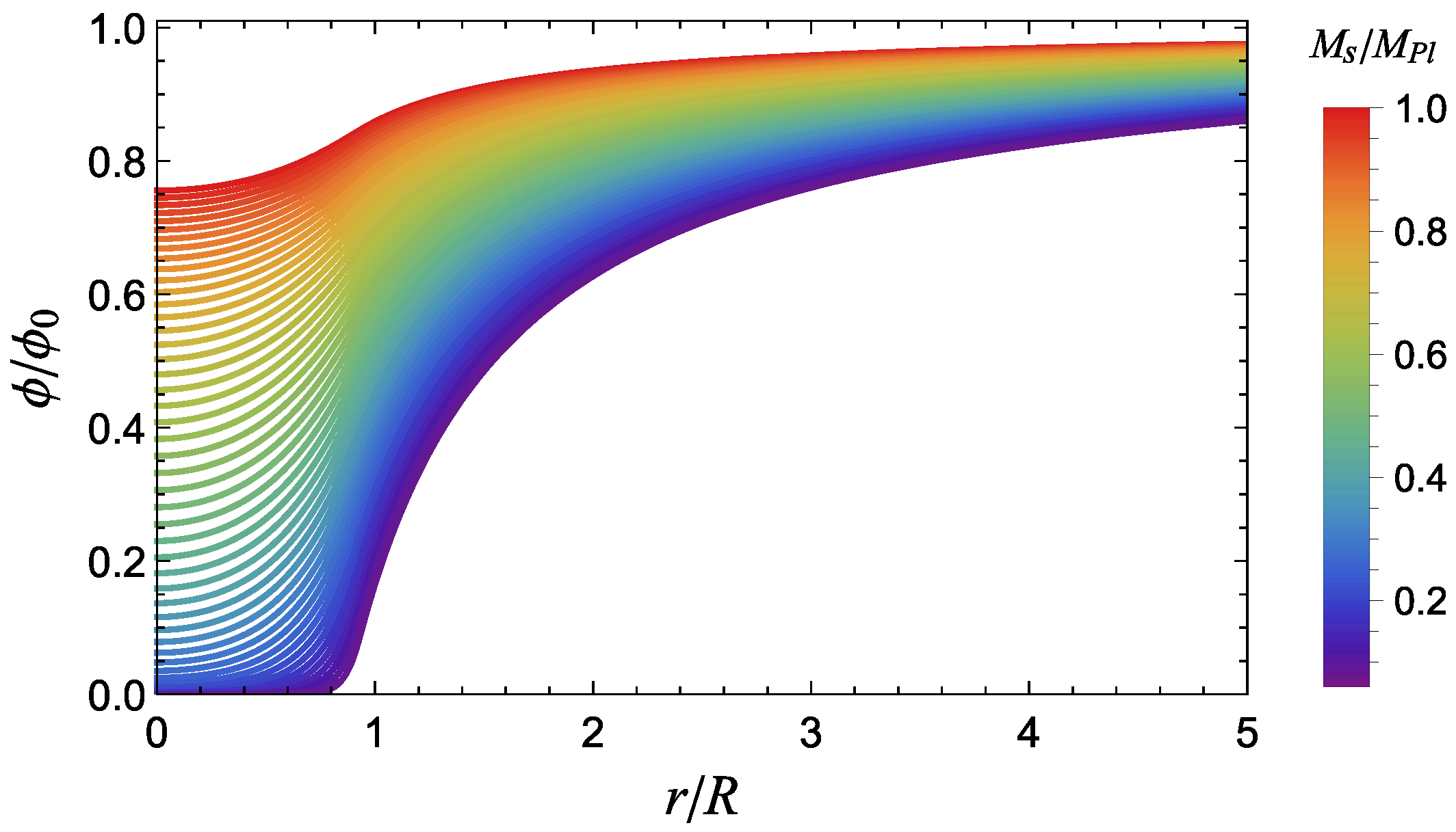
2.2. Screening
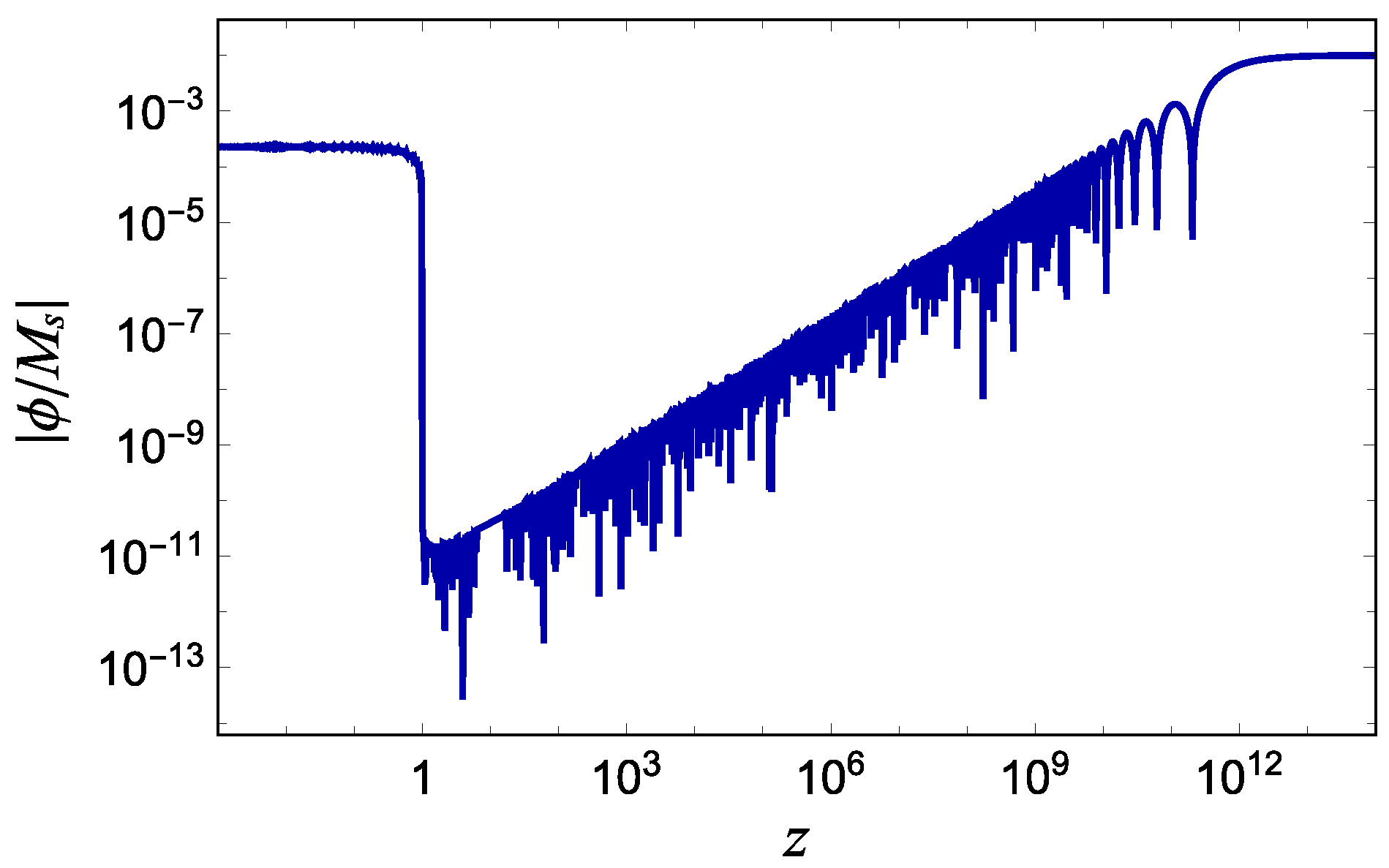
2.3. Cosmology
3. Equilibrium and Stability Properties of Symmetron Neutron Stars
3.1. Set-Up
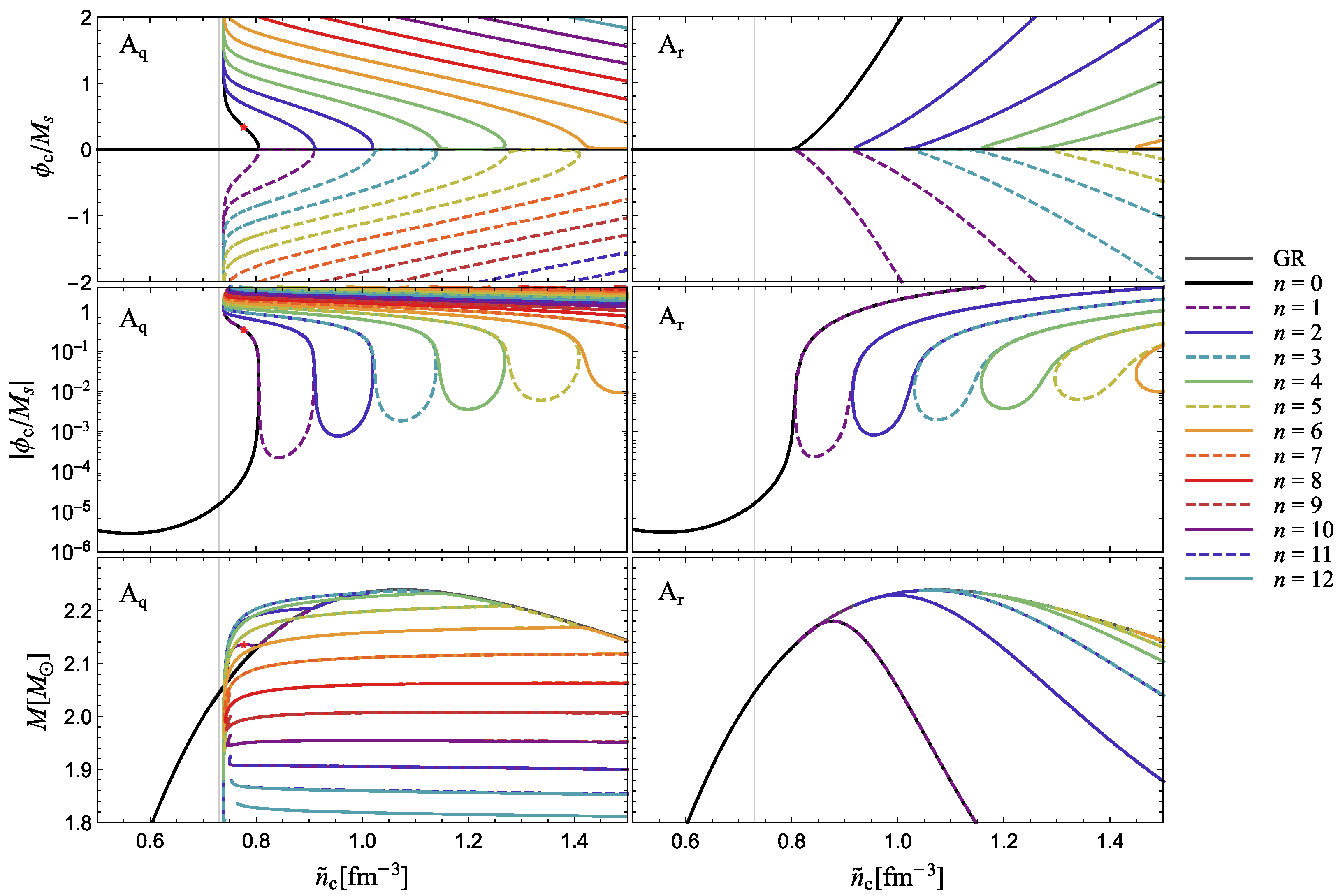
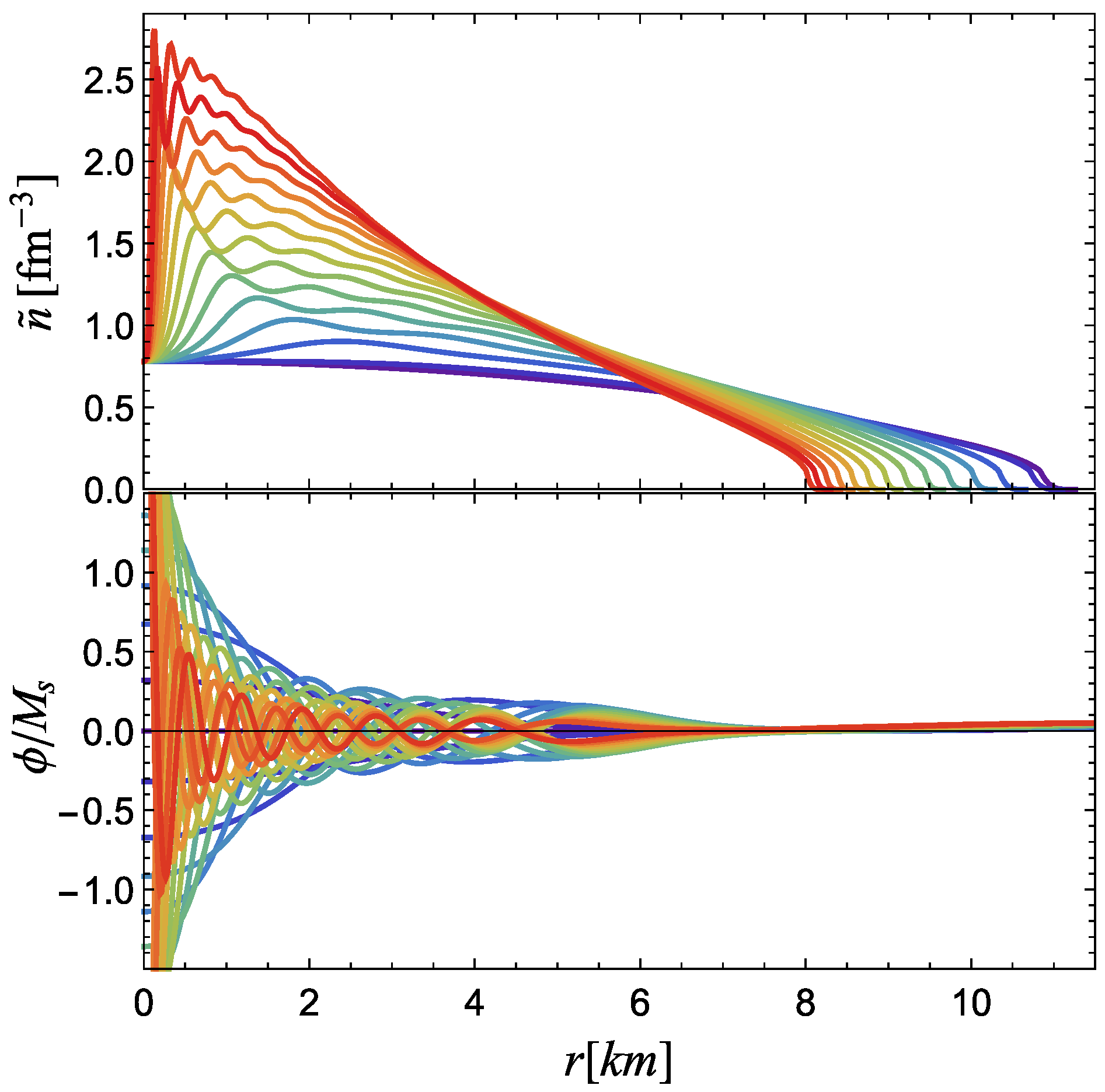
3.2. Symmetron Neutron Stars
4. Conclusions
Author Contributions
Funding
Data Availability Statement
Conflicts of Interest
| 1 | Explicit expressions for and are available at https://bitbucket.org/raissafpmendes/symmetron_neutron_stars.git (accessed on 30 November 2021). |
References
- Özel, F.; Freire, P. Masses, Radii, and the Equation of State of Neutron Stars. Annu. Rev. Astron. Astrophys. 2016, 54, 401–440. [Google Scholar] [CrossRef]
- Abbott, B.P.; Abbott, R.; Abbott, T.; Abraham, S.; Acernese, F.; Ackley, K.; Adams, C.; Adhikari, R.X.; Adya, V.B.; Affeldt, C.; et al. GWTC-1: A Gravitational-Wave Transient Catalog of Compact Binary Mergers Observed by LIGO and Virgo during the First and Second Observing Runs. Phys. Rev. X 2019, 9, 031040. [Google Scholar] [CrossRef]
- Abbott, R.; Abbott, T.D.; Abraham, S.; Acernese, F.; Ackley, K.; Adams, A.; Adams, C.; Adhikari, R.X.; Adya, V.B.; Affeldt, C.; et al. GWTC-2: Compact Binary Coalescences Observed by LIGO and Virgo during the First Half of the Third Observing Run. Phys. Rev. X 2021, 11, 021053. [Google Scholar] [CrossRef]
- Abbott, R.; Abbott, T.D.; Acernese, F.; Ackley, K.; Adams, C.; Adhikari, N.; Adhikari, R.X.; Adya, V.B.; Affeldt, C.; Agarwal, D.; et al. GWTC-3: Compact Binary Coalescences Observed by LIGO and Virgo During the Second Part of the Third Observing Run. arXiv 2021, arXiv:2111.03606. [Google Scholar]
- Pietroni, M. Dark energy condensation. Phys. Rev. D 2005, 72, 043535. [Google Scholar] [CrossRef]
- Olive, K.A.; Pospelov, M. Environmental dependence of masses and coupling constants. Phys. Rev. D 2008, 77, 043524. [Google Scholar] [CrossRef]
- Khoury, J. Theories of Dark Energy with Screening Mechanisms. arXiv 2010, arXiv:1011.5909. [Google Scholar]
- Damour, T.; Esposito-Farèse, G. Tensor-multi-scalar theories of gravitation. Class. Quantum Gravity 1992, 9, 2093–2176. [Google Scholar] [CrossRef]
- Damour, T.; Polyakov, A.M. The string dilation and a least coupling principle. Nucl. Phys. B 1994, 423, 532–558. [Google Scholar] [CrossRef]
- Baker, T.; Barreira, A.; Desmond, H.; Ferreira, P.; Jain, B.; Koyama, K.; Li, B.; Lombriser, L.; Nicola, A.; Sakstein, J.; et al. Novel Probes Project: Tests of gravity on astrophysical scales. Rev. Mod. Phys. 2021, 93, 015003. [Google Scholar] [CrossRef]
- Koyama, K. Cosmological tests of modified gravity. Rep. Prog. Phys. 2016, 79, 046902. [Google Scholar] [CrossRef] [PubMed]
- Bull, P.; Akrami, Y.; Adamek, J.; Baker, T.; Bellini, E.; Beltrán Jiménez, J.; Bentivegna, E.; Camera, S.; Clesse, S.; Davis, J.H.; et al. Beyond Λ CDM: Problems, solutions, and the road ahead. Phys. Dark Universe 2016, 12, 56–99. [Google Scholar] [CrossRef]
- Clifton, T.; Ferreira, P.G.; Padilla, A.; Skordis, C. Modified gravity and cosmology. Phys. Rep. 2012, 513, 1–189. [Google Scholar] [CrossRef]
- Joyce, A.; Jain, B.; Khoury, J.; Trodden, M. Beyond the cosmological standard model. Phys. Rep. 2015, 568, 1–98. [Google Scholar] [CrossRef]
- Will, C.M. The confrontation between general relativity and experiment. Living Rev. Relativ. 2006, 9, 4. [Google Scholar] [CrossRef] [PubMed]
- Sakstein, J. Astrophysical tests of screened modified gravity. Int. J. Mod. Phys. D 2018, 27, 1848008. [Google Scholar] [CrossRef]
- Khoury, J.; Weltman, A. Chameleon cosmology. Phys. Rev. D 2004, 69, 044026. [Google Scholar] [CrossRef]
- Khoury, J.; Weltman, A. Chameleon Fields: Awaiting Surprises for Tests of Gravity in Space. Phys. Rev. Lett. 2004, 93, 171104. [Google Scholar] [CrossRef]
- Hinterbichler, K.; Khoury, J. Screening Long-Range Forces through Local Symmetry Restoration. Phys. Rev. Lett. 2010, 104, 231301. [Google Scholar] [CrossRef]
- Hinterbichler, K.; Khoury, J.; Levy, A.; Matas, A. Symmetron cosmology. Phys. Rev. D 2011, 84, 103521. [Google Scholar] [CrossRef]
- Brax, P.; Davis, A.C.; Li, B.; Winther, H.A. Unified description of screened modified gravity. Phys. Rev. D 2012, 86, 044015. [Google Scholar] [CrossRef]
- Brax, P.; Davis, A.C.; Li, B. Modified gravity tomography. Phys. Lett.s B 2012, 715, 38–43. [Google Scholar] [CrossRef]
- Burrage, C.; Copeland, E.J.; Millington, P. Radiative Screening of Fifth Forces. Phys. Rev. Lett. 2016, 117, 211102. [Google Scholar] [CrossRef]
- Dong, R.; Kinney, W.H.; Stojkovic, D. Symmetron inflation. J. Cosmol. Astropart. Phys. 2014, 2014, 021. [Google Scholar] [CrossRef]
- Brax, P.; van de Bruck, C.; Davis, A.C.; Li, B.; Schmauch, B.; Shaw, D.J. Linear growth of structure in the symmetron model. Phys. Rev. D 2011, 84, 123524. [Google Scholar] [CrossRef]
- Brax, P.; Davis, A.C.; Li, B.; Winther, H.A.; Zhao, G.B. Systematic simulations of modified gravity: Symmetron and dilaton models. J. Cosmol. Astropart. Phys. 2012, 2012, 002. [Google Scholar] [CrossRef]
- Davis, A.C.; Li, B.; Mota, D.F.; Winther, H.A. Structure formation in the symmetron model. Astrophys. J. 2012, 748, 61. [Google Scholar] [CrossRef]
- Llinares, C.; Mota, D.F. Releasing Scalar Fields: Cosmological Simulations of Scalar-Tensor Theories for Gravity Beyond the Static Approximation. Phys. Rev. Lett. 2013, 110, 161101. [Google Scholar] [CrossRef]
- Llinares, C.; Mota, D.F. Cosmological simulations of screened modified gravity out of the static approximation: Effects on matter distribution. Phys. Rev. D 2014, 89, 084023. [Google Scholar] [CrossRef]
- Mota, D.F. Probing screened modified gravity with nonlinear structure formation. Int. J. Mod. Phys. D 2018, 27, 1830003. [Google Scholar] [CrossRef]
- Clampitt, J.; Jain, B.; Khoury, J. Halo scale predictions of symmetron modified gravity. J. Cosmol. Astropart. Phys. 2012, 2012, 030. [Google Scholar] [CrossRef]
- Taddei, L.; Catena, R.; Pietroni, M. Spherical collapse and halo mass function in the symmetron model. Phys. Rev. D 2014, 89, 023523. [Google Scholar] [CrossRef]
- Contigiani, O.; Vardanyan, V.; Silvestri, A. Splashback radius in symmetron gravity. Phys. Rev. D 2019, 99, 064030. [Google Scholar] [CrossRef]
- Burrage, C.; Copeland, E.J.; Millington, P. Radial acceleration relation from symmetron fifth forces. Phys. Rev. D 2017, 95, 064050. [Google Scholar] [CrossRef]
- O’Hare, C.A.J.; Burrage, C. Stellar kinematics from the symmetron fifth force in the Milky Way disk. Phys. Rev. D 2018, 98, 064019. [Google Scholar] [CrossRef]
- Burrage, C.; Copeland, E.J.; Käding, C.; Millington, P. Symmetron scalar fields: Modified gravity, dark matter, or both? Phys. Rev. D 2019, 99, 043539. [Google Scholar] [CrossRef]
- Upadhye, A. Symmetron Dark Energy in Laboratory Experiments. Phys. Rev. Lett. 2013, 110, 031301. [Google Scholar] [CrossRef]
- Burrage, C.; Kuribayashi-Coleman, A.; Stevenson, J.; Thrussell, B. Constraining symmetron fields with atom interferometry. J. Cosmol. Astropart. Phys. 2016, 2016, 041. [Google Scholar] [CrossRef]
- Cronenberg, G.; Brax, P.; Filter, H.; Geltenbort, P.; Jenke, T.; Pignol, G.; Pitschmann, M.; Thalhammer, M.; Abele, H. Acoustic Rabi oscillations between gravitational quantum states and impact on symmetron dark energy. Nat. Phys. 2018, 14, 1022–1026. [Google Scholar] [CrossRef]
- Chiow, S.w.; Yu, N. Constraining symmetron dark energy using atom interferometry. Phys. Rev. D 2020, 101, 083501. [Google Scholar] [CrossRef]
- Elder, B.; Vardanyan, V.; Akrami, Y.; Brax, P.; Davis, A.C.; Decca, R.S. Classical symmetron force in Casimir experiments. Phys. Rev. D 2020, 101, 064065. [Google Scholar] [CrossRef]
- Burrage, C.; Sakstein, J. Tests of chameleon gravity. Living Rev. Relativ. 2018, 21, 1. [Google Scholar] [CrossRef] [PubMed]
- Babichev, E.; Langlois, D. Relativistic stars in f(R) and scalar-tensor theories. Phys. Rev. D 2010, 81, 124051. [Google Scholar] [CrossRef]
- Brax, P.; Davis, A.C.; Jha, R. Neutron stars in screened modified gravity: Chameleon versus dilaton. Phys. Rev. D 2017, 95, 083514. [Google Scholar] [CrossRef]
- De Aguiar, B.F.; Mendes, R.F.P. Highly compact neutron stars and screening mechanisms: Equilibrium and stability. Phys. Rev. D 2020, 102, 024064. [Google Scholar] [CrossRef]
- Podkowka, D.M.; Mendes, R.F.P.; Poisson, E. Trace of the energy-momentum tensor and macroscopic properties of neutron stars. Phys. Rev. D 2018, 98, 064057. [Google Scholar] [CrossRef]
- Saes, J.; Mendes, R.F.P. An equation-of-state-insensitive measure of neutron star stiffness. arXiv 2021, arXiv:2109.11571. [Google Scholar]
- Dima, A.; Bezares, M.; Barausse, E. Dynamical chameleon neutron stars: Stability, radial oscillations, and scalar radiation in spherical symmetry. Phys. Rev. D 2021, 104, 084017. [Google Scholar] [CrossRef]
- Jain, B.; Vikram, V.; Sakstein, J. Astrophysical tests of modified gravity: Constraints from distance indicators in the nearby universe. Astrophys. J. 2013, 779, 39. [Google Scholar] [CrossRef]
- Engvik, L.; Osnes, E.; Hjorth-Jensen, M.; Bao, G.; Ostgaard, E. Asymmetric Nuclear Matter and Neutron Star Properties. Astrophys. J. 1996, 469, 794. [Google Scholar] [CrossRef]
- Read, J.; Lackey, B.; Owen, B.; Friedman, J.L. Constraints on a phenomenologically parametrized neutron-star equation of state. Phys. Rev. D 2009, 79, 124032. [Google Scholar] [CrossRef]
- Mendes, R.F.P.; Ortiz, N. Highly compact neutron stars in scalar-tensor theories of gravity: Spontaneous scalarization versus gravitational collapse. Phys. Rev. D 2016, 93, 124035. [Google Scholar] [CrossRef]
- Palenzuela, C.; Liebling, S.L. Constraining scalar-tensor theories of gravity from the most massive neutron stars. Phys. Rev. D 2016, 93, 044009. [Google Scholar] [CrossRef]
- Damour, T.; Esposito-Farèse, G. Nonperturbative strong-field effects in tensor-scalar theories of gravitation. Phys. Rev. Lett. 1993, 70, 2220–2223. [Google Scholar] [CrossRef] [PubMed]
- Salgado, M.; Sudarsky, D.; Nucamendi, U. Spontaneous scalarization. Phys. Rev. D 1998, 58, 124003. [Google Scholar] [CrossRef]
- Harada, T. Neutron stars in scalar-tensor theories of gravity and catastrophe theory. Phys. Rev. D 1998, 57, 4802–4811. [Google Scholar] [CrossRef]
- Harada, T. Stability Analysis of Spherically Symmetric Star in Scalar-Tensor Theories of Gravity. Prog. Theor. Phys. 1997, 98, 359–379. [Google Scholar] [CrossRef]
- Mendes, R.F.P. Possibility of setting a new constraint to scalar-tensor theories. Phys. Rev. D 2015, 91, 064024. [Google Scholar] [CrossRef]
- Rosca-Mead, R.; Moore, C.J.; Sperhake, U.; Agathos, M.; Gerosa, D. Structure of Neutron Stars in Massive Scalar-Tensor Gravity. Symmetry 2020, 12, 1384. [Google Scholar] [CrossRef]
- Pani, P.; Cardoso, V.; Berti, E.; Read, J.; Salgado, M. Vacuum revealed: The final state of vacuum instabilities in compact stars. Phys. Rev. D 2011, 83, 081501. [Google Scholar] [CrossRef]


Publisher’s Note: MDPI stays neutral with regard to jurisdictional claims in published maps and institutional affiliations. |
© 2021 by the authors. Licensee MDPI, Basel, Switzerland. This article is an open access article distributed under the terms and conditions of the Creative Commons Attribution (CC BY) license (https://creativecommons.org/licenses/by/4.0/).
Share and Cite
de Aguiar, B.F.; Mendes, R.F.P.; Falciano, F.T. Neutron Stars in the Symmetron Model. Universe 2022, 8, 6. https://doi.org/10.3390/universe8010006
de Aguiar BF, Mendes RFP, Falciano FT. Neutron Stars in the Symmetron Model. Universe. 2022; 8(1):6. https://doi.org/10.3390/universe8010006
Chicago/Turabian Stylede Aguiar, Bernardo F., Raissa F. P. Mendes, and Felipe T. Falciano. 2022. "Neutron Stars in the Symmetron Model" Universe 8, no. 1: 6. https://doi.org/10.3390/universe8010006
APA Stylede Aguiar, B. F., Mendes, R. F. P., & Falciano, F. T. (2022). Neutron Stars in the Symmetron Model. Universe, 8(1), 6. https://doi.org/10.3390/universe8010006