
Design of New Resonant Haloscopes in the Search for the Dark Matter Axion: A Review of the First Steps in the RADES Collaboration

 ,
,  ,
,  , ,
, ,  , , , ,
Abstract
1. Introduction
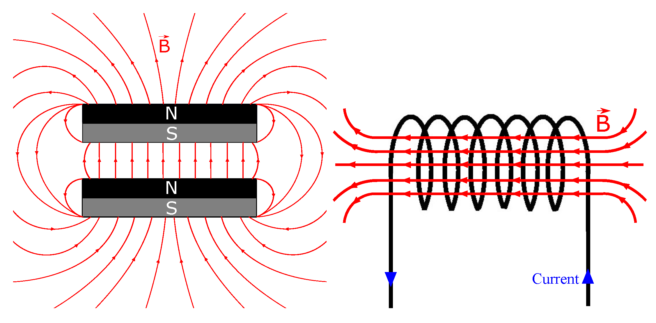
2. General Principles in Resonant Haloscope Design
2.1. Detected Power
2.2. Axion Coupling Sensitivity
2.3. Scanning Rate
3. Motivation and Constraints of the RADES Project
3.1. First Attempt: Increasing the Length of the Cavity
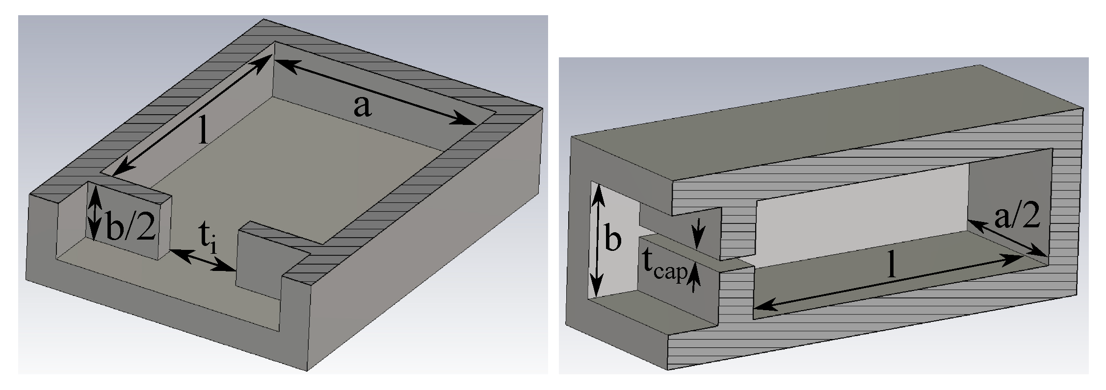
3.2. The Alternative: Multi-Cavity Concept

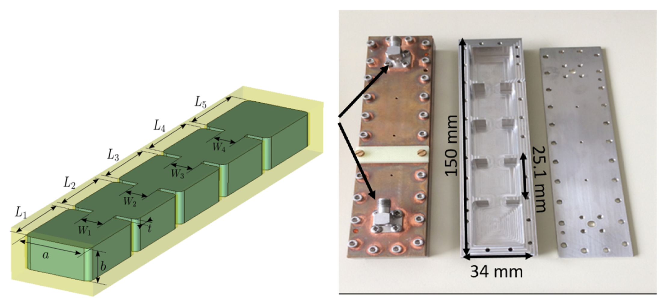
4. First Multi-Cavity Haloscopes
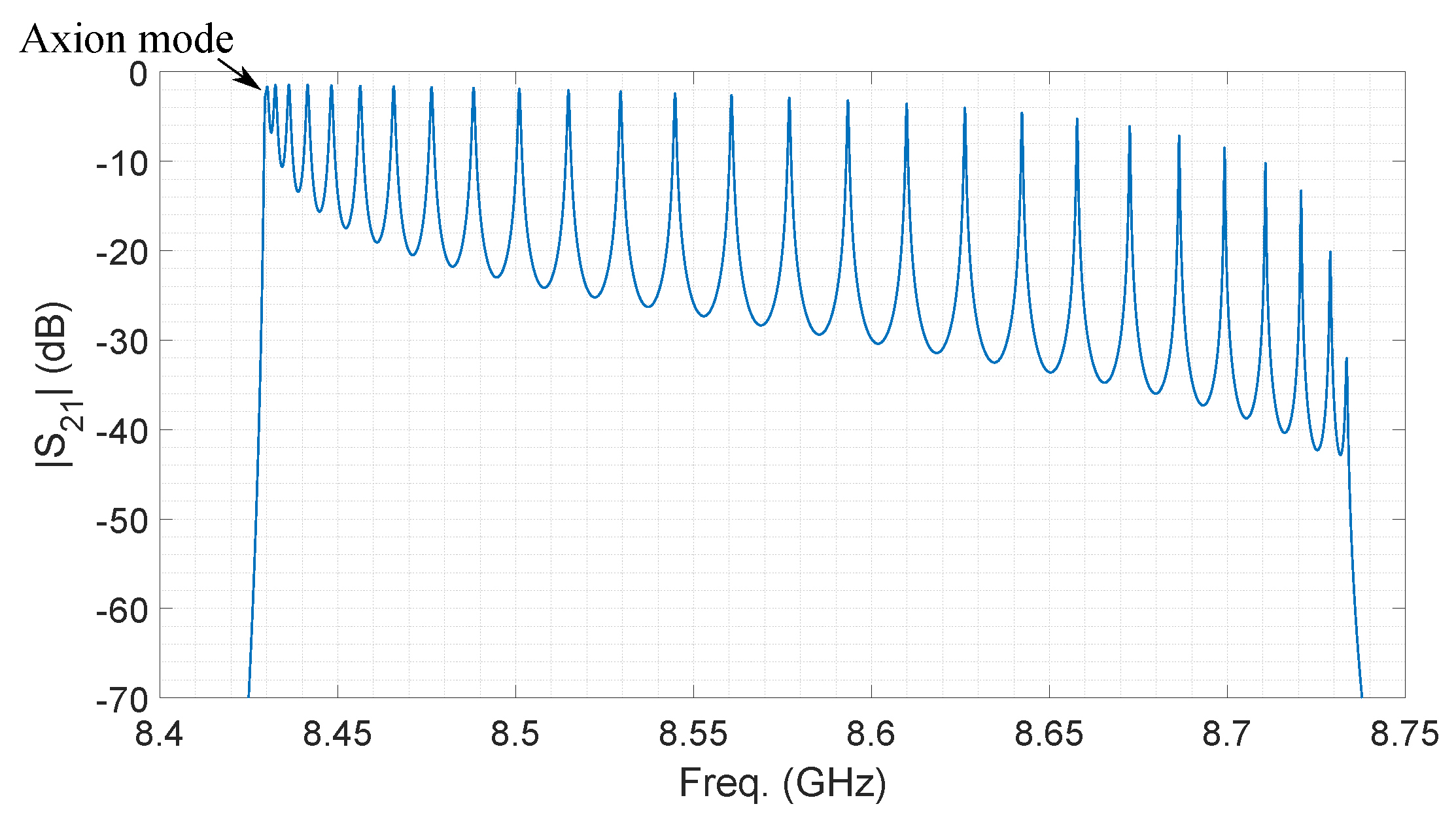
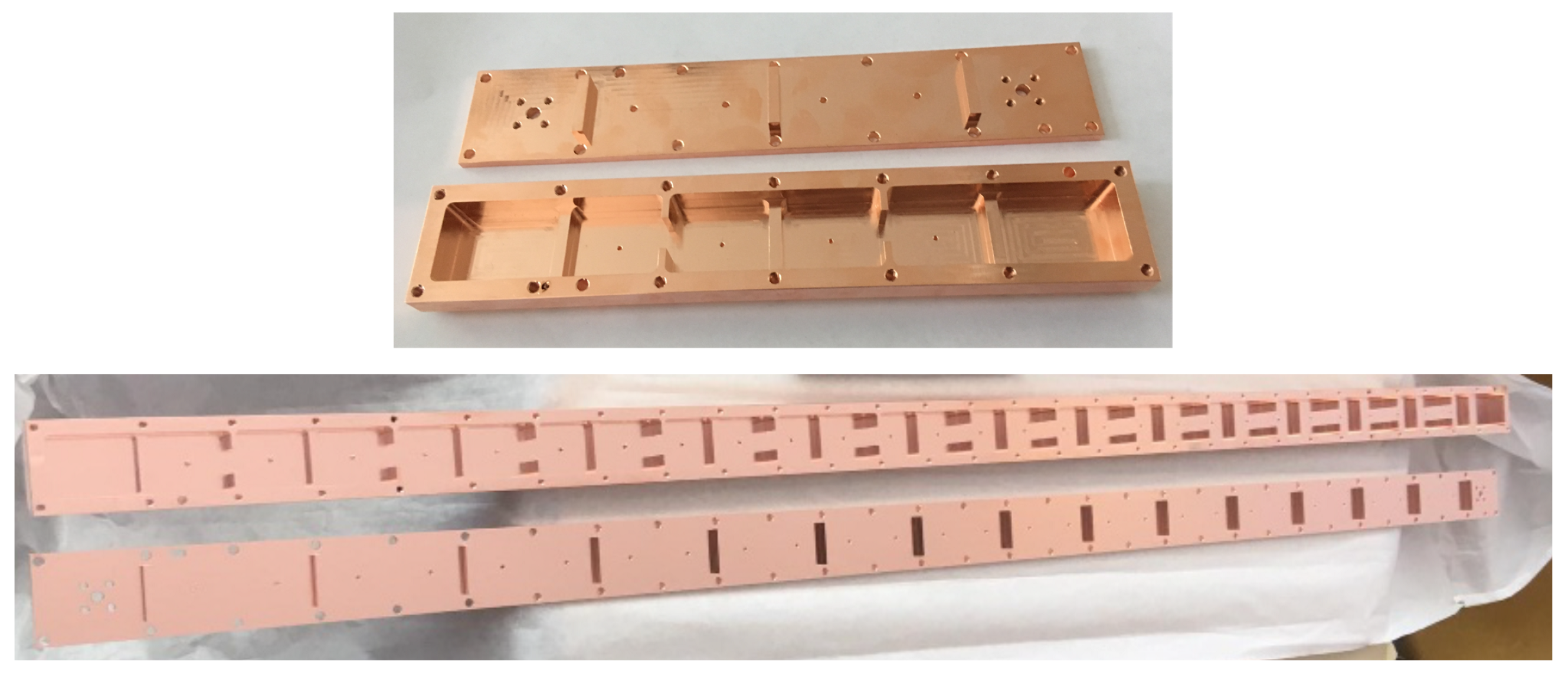
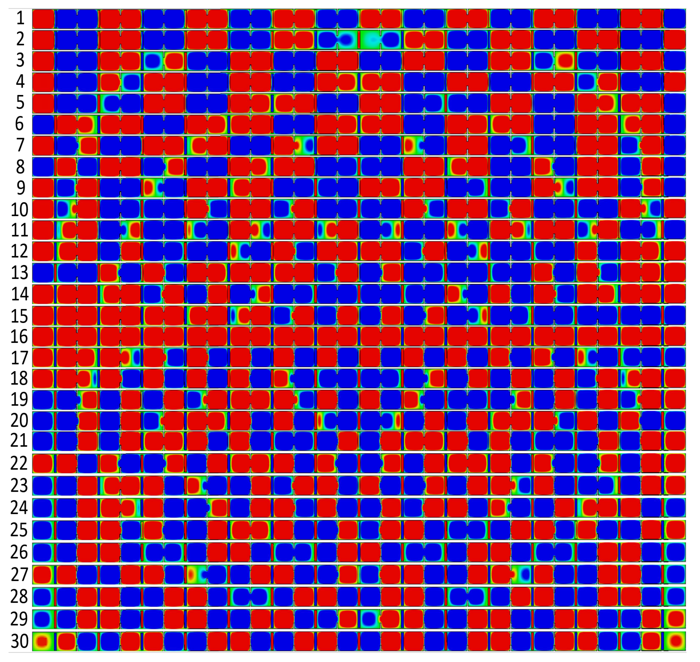
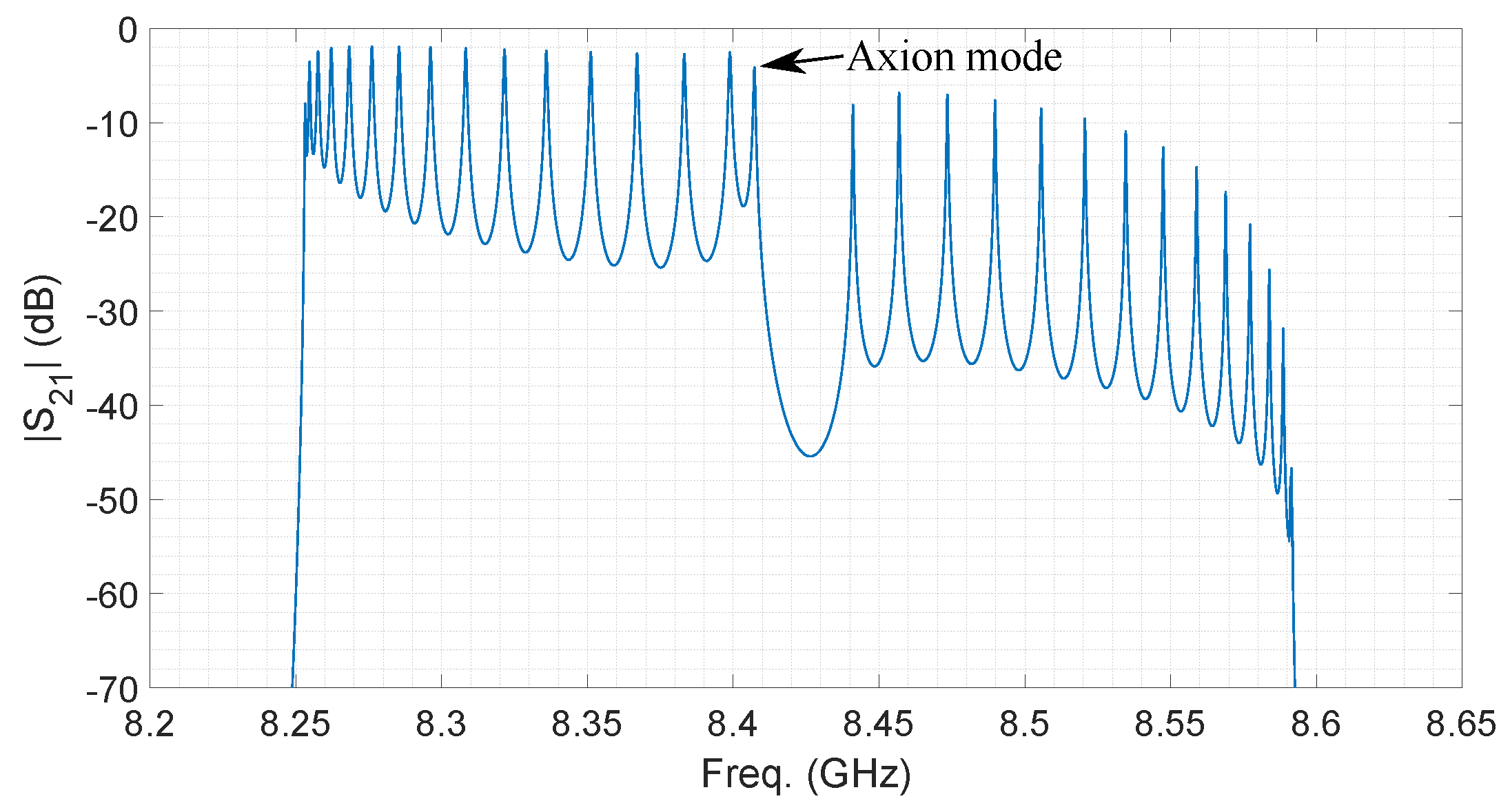
4.1. All Inductive 5-Cavity Haloscope
4.2. Alternate Coupling
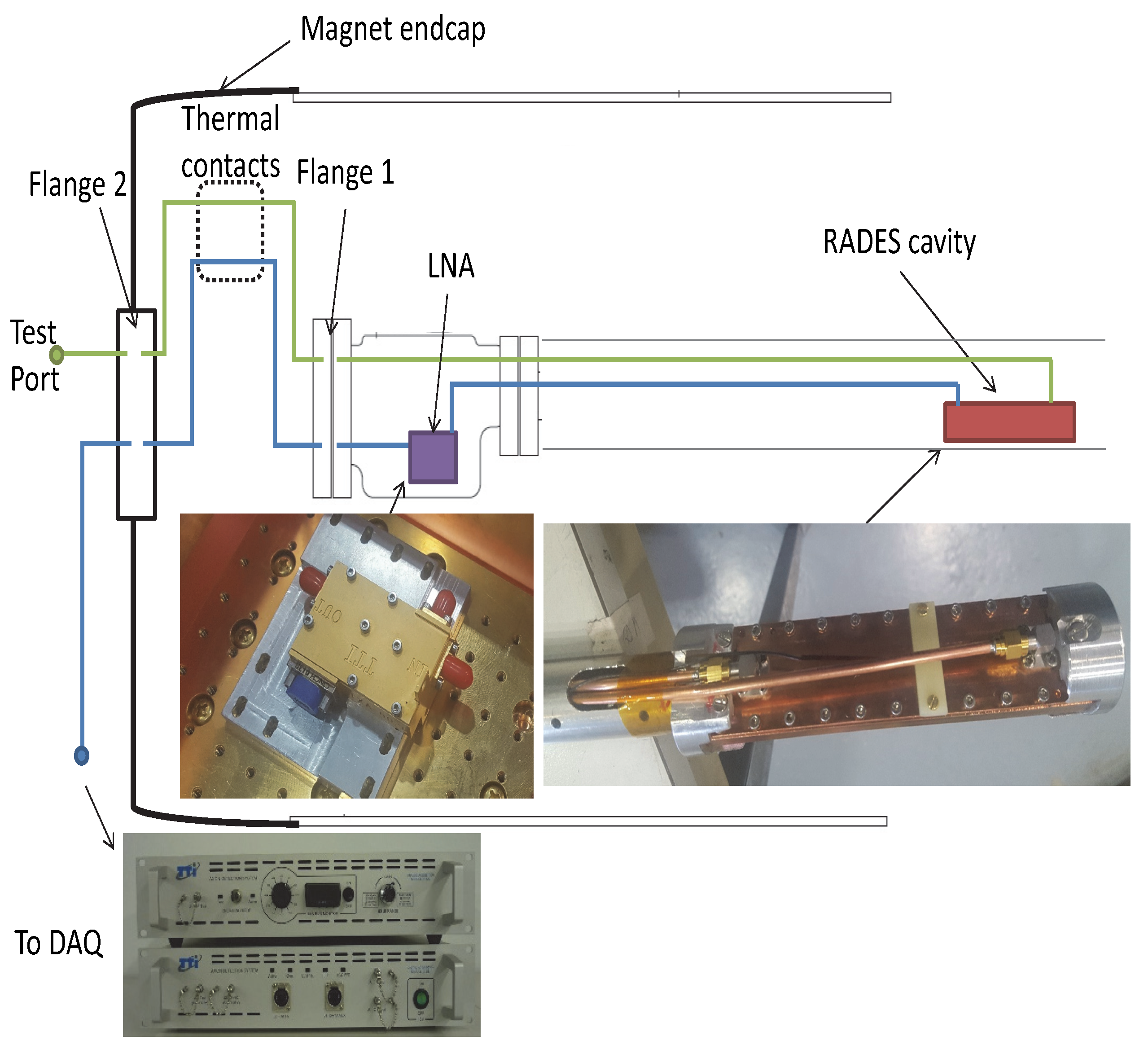
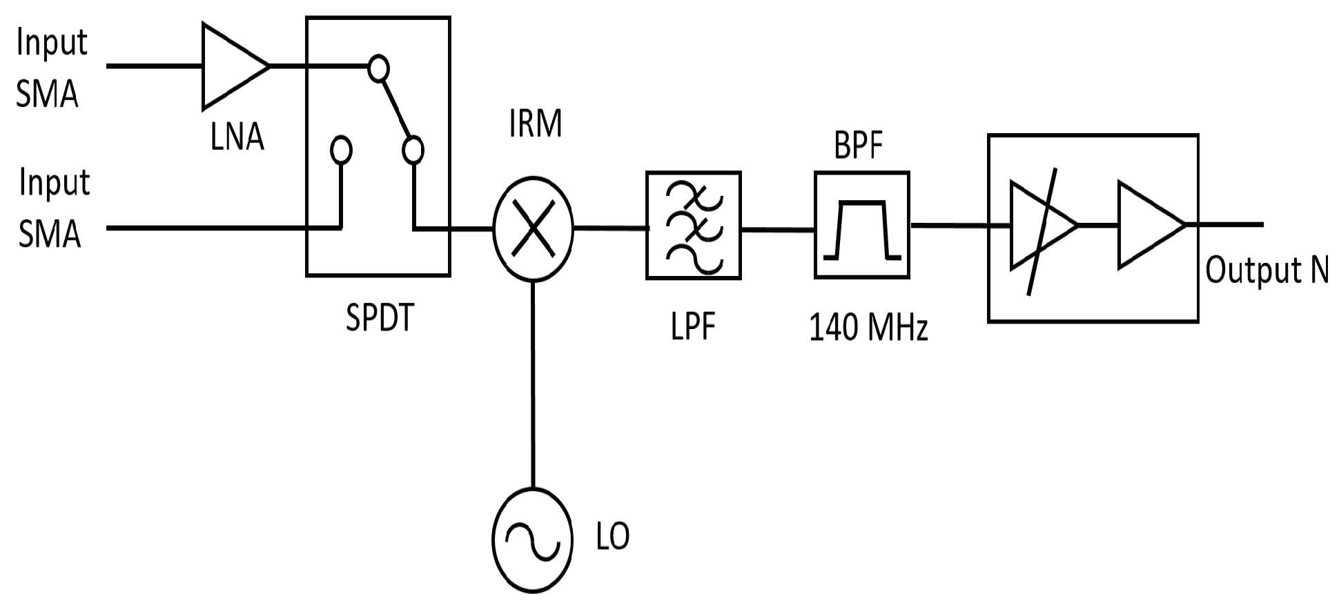
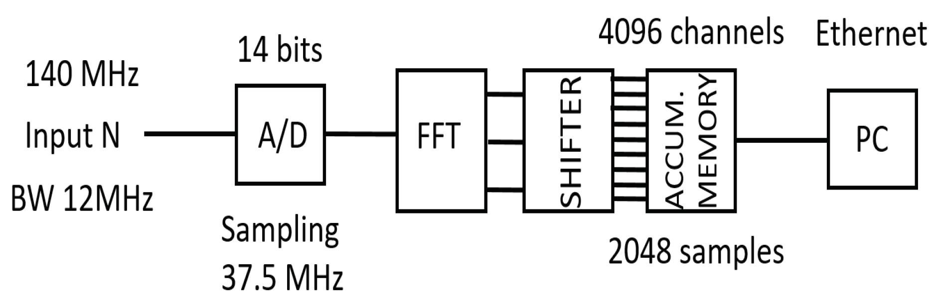
5. Data Acquisition System
- RF LNA: It amplified the input RF signal. It worked from 8 GHz to 9 GHz and provided a gain around 55 dB and 30 dB input return loss.
- Single pole double through (SPDT) RF switch: This device allowed us to visualize the amplified RF signal at the test output port, or to directly check the down converter circuit.
- Down converter: It down-converted the input signal from X band to a frequency band around 140 MHz. It was an image rejection mixer (IRM) which provided 26 dB of image band rejection.
- Local oscillator (LO): It provided the frequency signal to convert the RF input signal to the 140 MHz band. Its working power level was 0 dBm working from 7860 to 8860 MHz.
- IF filtering: This section filtered the desired IF signal from 134 MHz to 146 MHz. It consisted of two filters in series: a low pass filter (LPF) to reject the LO leakage from the IRM, and a surface acoustic wave (SAW) band pass filter (BPF) to select the wanted IF frequency band.
- IF signal conditioning: This module amplified or attenuated the IF signal to provide the desired IF output level. Its function was to bring the IF signal to the best input level for the digital acquisition module. The amplification or attenuation level depended on the input RF signal power.
- Power supply unit: This unit fed all the modules that formed the analog acquisition module.
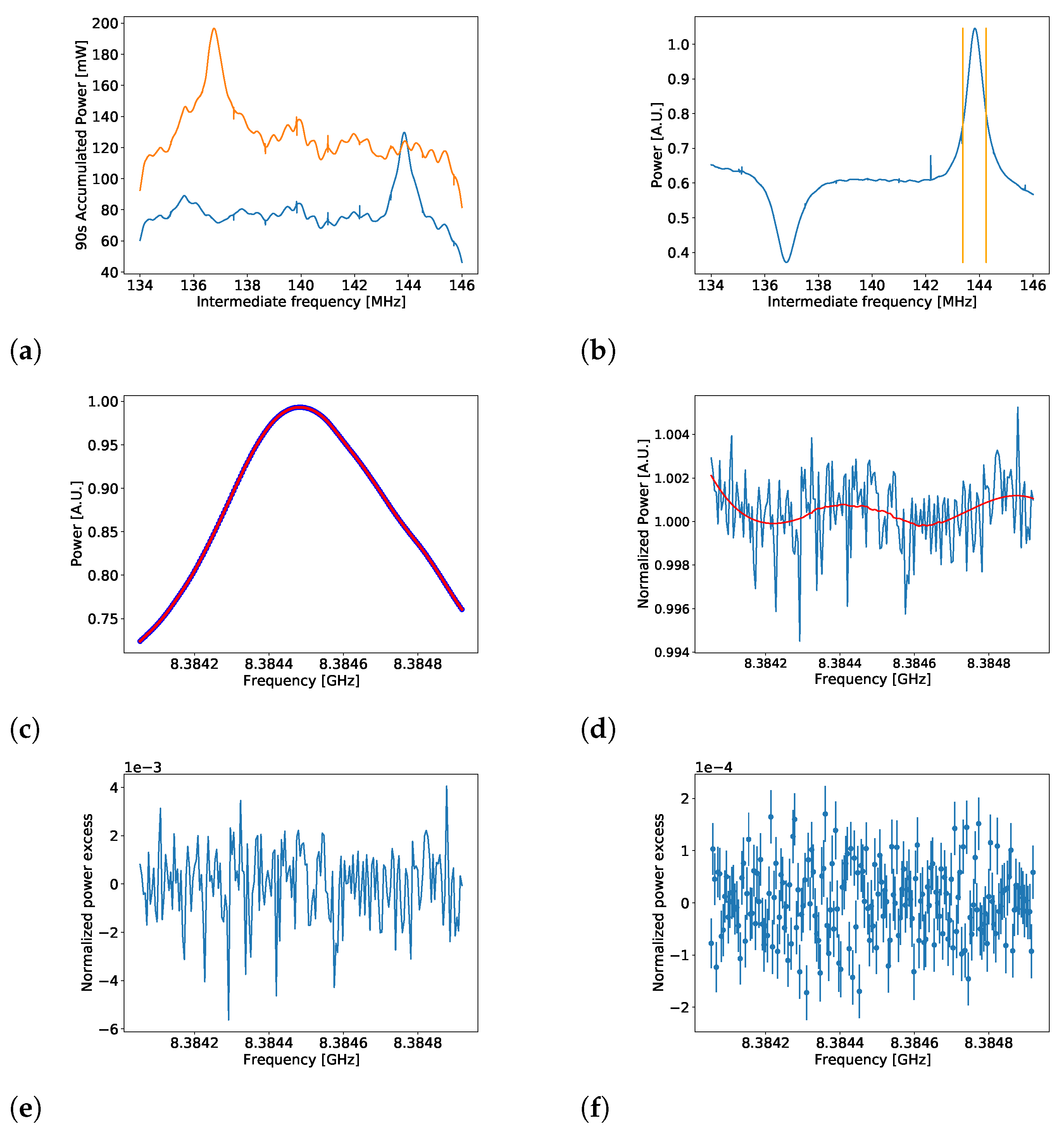
6. First Results
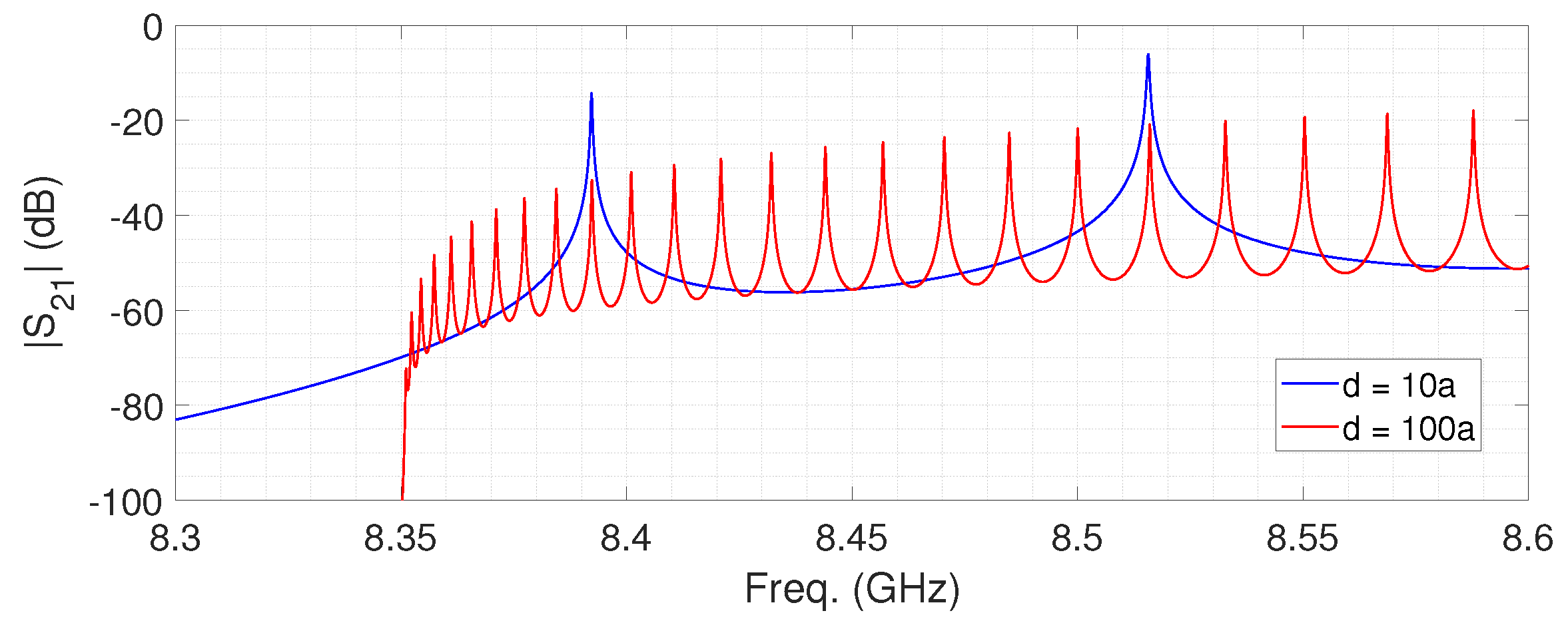
- Dividing each 90s spectrum taken at by the average spectrum of . This was a first-order correction to the electronic background introduced by the DAQ (see Figure 17b).
- Limiting the frequency region of the analysis to a range of ∼ 0.87 MHz around the resonance peak (see Figure 17b). This range covered more than the full width at half maximum of the Lorentzian peak.
- Normalized spectra were created by dividing each 90s spectrum by the SG-fit (see Figure 17d).
- Due to drifts in the receiver chain, the normalized spectra still had unwanted structure remaining within the spectra. A second SG-fit (SG*) was created for each normalized 90s spectrum. The spectra were divided by the SG*-fits, and the result was subtracted by 1 to create unit-less normalized power spectra (see Figure 17e).
- The unit-less normalized power spectra were combined into a grand unified spectrum.
- The previous steps were repeated for the magnet-off data sets.
- The final spectrum was the difference of the magnet-on and magnet-off grand unified spectra (see Figure 17f).

7. Envisaged Work
7.1. Increasing the Experiment’s Sensitivity
7.2. Haloscopes for Other Frequencies
7.3. Developments in Numerical Simulation: Application of the BI-RME 3D Method to Axion-Photon Coupling in Resonant Cavities
8. Conclusions
Author Contributions
Funding
Data Availability Statement
Conflicts of Interest
| 1 | To measure the cavity coupling, an RF switch was installed after the data taking. Bypassing the LNA was thus not possible during data taking. The measured after the installation of the switch was similar to the one computed during the data-taking period. From this result it can be assumed that the coupling measured before and after the data-taking period were the same. |
References
- Peccei, R.D.; Quinn, H.R. CP conservation in the presence of pseudoparticles. Phys. Rev. Lett. 1977, 38, 1440–1443. [Google Scholar] [CrossRef]
- Peccei, R.D.; Quinn, H.R. Constraints imposed by CP conservation in the presence of pseudoparticles. Phys. Rev. D 1977, 16, 1791–1797. [Google Scholar] [CrossRef]
- Weinberg, S. A new light boson? Phys. Rev. Lett. 1978, 40, 223–226. [Google Scholar] [CrossRef]
- Wilczek, F. Problem of strong P and T invariance in the presence of instantons. Phys. Rev. Lett. 1978, 40, 279–282. [Google Scholar] [CrossRef]
- Preskill, J.; Wise, M.B.; Wilczek, F. Cosmology of the Invisible Axion. Phys. Lett. B 1983, 120, 127–132. [Google Scholar] [CrossRef]
- Abbott, L.F.; Sikivie, P. A Cosmological Bound on the Invisible Axion. Phys. Lett. B 1983, 120, 133–136. [Google Scholar] [CrossRef]
- Dine, M.; Fischler, W. The Not So Harmless Axion. Phys. Lett. B 1983, 120, 137–141. [Google Scholar] [CrossRef]
- Primakoff, H. Photoproduction of neutral mesons in nuclear electric fields and the mean life of the neutral meson. Phys. Rev. 1951, 81, 899. [Google Scholar] [CrossRef]
- Sikivie, P. Experimental Tests of the Invisible Axion. Phys. Rev. Lett. 1983, 51, 1415–1417, Erratum in Phys. Rev. Lett. 1984, 52, 695. [Google Scholar] [CrossRef]
- Bibber, K.V.; Dagdeviren, N.R.; Koonin, S.E.; Kerman, A.K.; Nelson, H.N. Proposed experiment to produce and detect light pseudoscalars. Phys. Rev. Lett. 1987, 59, 759–762. [Google Scholar] [CrossRef]
- Fukuda, Y.; Kohmoto, T.; Nakajima, S.; Kunitomo, M. Production and detection of axions by using optical resonators. Prog. Cryst. Growth Charact. Mater. 1996, 33, 363–366. [Google Scholar] [CrossRef]
- Sikivie, P.; Tanner, D.B.; Bibber, K. Resonantly enhanced axion-photon regeneration. Phys. Rev. Lett. 2007, 98, 172002. [Google Scholar] [CrossRef]
- Lazarus, D.M.; Smith, G.C.; Cameron, R.; Melissinos, A.C.; Ruoso, G.; Semertzidis, Y.K.; Nezrick, F.A. Search for solar axions. Phys. Rev. Lett. 1992, 69, 2333–2336. [Google Scholar] [CrossRef] [PubMed]
- Inoue, Y.; Namba, T.; Moriyama, S.; Minowa, M.; Takasu, Y.; Horiuchi, T.; Yamamoto, A. Search for sub-electronvolt solar axions using coherent conversion of axions into photons in magnetic field and gas helium. Phys. Lett. B 2002, 536, 18–23. [Google Scholar] [CrossRef]
- Moriyama, S.; Minowa, M.; Namba, T.; Inoue, Y.; Takasu, Y.; Yamamoto, A. Direct search for solar axions by using strong magnetic field and X-ray detectors. Phys. Lett. B 1998, 434, 147–152. [Google Scholar] [CrossRef]
- Inoue, Y.; Akimoto, Y.; Ohta, R.; Mizumoto, T.; Yamamoto, A.; Minowa, M. Search for solar axions with mass around 1 eV using coherent conversion of axions into photons. Phys. Lett. B 2008, 668, 93–97. [Google Scholar] [CrossRef]
- Anastassopoulos, V.; Aune, S.; Barth, K.; Belov, A.; Bräuninger, H.; Cantatore, G.; Carmona, J.M.; Castel, J.F.; Cetin, S.A.; Christensen, F.; et al. New CAST limit on the axion–photon interaction. Nat. Phys. 2017, 13, 584–590. [Google Scholar] [CrossRef]
- Arik, M.; Aune, S.; Barth, K.; Belov, A.; Borghi, S.; Bräuninger, H.; Cantatore, G.; Carmona, J.M.; Cetin, S.A.; Collar, J.I.; et al. Search for Sub-eV Mass Solar Axions by the CERN Axion Solar Telescope with 3He Buffer Gas. Phys. Rev. Lett. 2011, 107, 261302. [Google Scholar] [CrossRef]
- Armengaud, E.; Attie, D.; Basso, S.; Brun, P.; Bykovskiy, N.; Carmona, J.M.; Castel, J.F.; Cebrián, S.; Cicoli, M.; Civitani, M.; et al. Physics potential of the International Axion Observatory (IAXO). J. Cosmol. Astropart. Phys. 2019, 047. [Google Scholar] [CrossRef]
- Graham, P.W.; Irastorza, I.G.; Lamoreaux, S.K.; Lindner, A.; Bibber, K.A. Experimental Searches for the Axion and Axion-Like Particles. Annu. Rev. Nucl. Part. Sci. 2015, 65, 485–514. [Google Scholar] [CrossRef]
- Irastorza, I.G.; Redondo, J. New experimental approaches in the search for axion-like particles. Prog. Part. Nucl. Phys. 2018, 102, 89–159. [Google Scholar] [CrossRef]
- Luzio, L.D.; Giannotti, M.; Nardi, E.; Visinelli, L. The landscape of QCD axion models. Phys. Rep. 2020, 870, 1–117. [Google Scholar] [CrossRef]
- Sikivie, P. Invisible axion search methods. Rev. Mod. Phys. 2021, 93, 015004. [Google Scholar] [CrossRef]
- Stern, I. ADMX Status. In Proceedings of the Science, 38th International Conference on High Energy Physics, Chicago, IL, USA, 3–10 August 2016. [Google Scholar]
- Wuensch, W.; De Panfilis-Wuensch, S.; Semertzidis, Y.K.; Rogers, J.T.; Melissinos, A.C.; Halama, H.J.; Moskowitz, B.E.; Prodell, A.G.; Fowler, W.B.; Nezrick, F.A. Results of a laboratory search for cosmic axions and other weakly coupled light particles. Phys. Rev. D 1989, 40, 3153. [Google Scholar] [CrossRef] [PubMed]
- Hagmann, C.; Sikivie, P.; Sullivan, N.S.; Tanner, D.B. Results from a search for cosmic axions. Phys. Rev. D 1990, 42, 1297. [Google Scholar] [CrossRef]
- Alesini, D.; Babusci, D.; Di Gioacchino, D.; Gatti, C.; Lamanna, G.; Ligi, C. The KLASH Proposal. arXiv 2017, arXiv:1707.06010. [Google Scholar]
- Kenany, S.A.; Anil, M.A.; Backes, K.M.; Brubaker, B.M.; Cahn, S.B.; Carosi, G.; Gurevich, Y.V.; Kindel, W.F.; Lamoreaux, S.K.; Lehnert, K.M.; et al. Design and operational experience of a microwave cavity axion detector for the 20–100 μeV range. Nucl. Instrum. Meth. A 2017, 854, 11–24. [Google Scholar] [CrossRef]
- McAllister, B.T.; Flower, G.; Ivanov, E.N.; Goryachev, M.; Bourhill, J.; Tobar, M.E. The ORGAN Experiment: An axion haloscope above 15 GHz. Phys. Dark Universe 2017, 18, 67–72. [Google Scholar] [CrossRef]
- Alesini, D.; Braggio, C.; Carugno, G.; Crescini, N.; D’Agostino, D.; Di Gioacchino, D.; Di Vora, R.; Falferi, P.; Gambardella, U.; Gatti, C.; et al. Search for invisible axion dark matter of mass ma = 43 μeV with the QUAX–aγ experiment. Phys. Rev. D 2021, 103, 102004. [Google Scholar] [CrossRef]
- Jeong, J.; Youn, S.; Ahn, S.; Kim, J.E.; Semertzidis, Y.K. Concept of multiple-cell cavity for axion dark matter search. Phys. Lett. B 2018, 777, 412–419. [Google Scholar] [CrossRef]
- Melcón, A.Á.; Arguedas Cuendis, S.; Cogollos, C.; Díaz-Morcillo, A.; Döbrich, B.; Gallego, J.D.; Gimeno, B.; Irastorza, I.G.; Lozano-Guerrero, A.J.; Malbrunot, C.; et al. Axion searches with microwave filters: The RADES project. J. Cosmol. Astropart. Phys. 2018, 2018, 040. [Google Scholar] [CrossRef]
- Kim, Y.; Kim, D.; Jeong, J.; Kim, J.; Shin, Y.C.; Semertzidis, Y.K. Effective approximation of electromagnetism for axion haloscope searches. Phys. Dark Universe 2019, 26, 100362. [Google Scholar] [CrossRef]
- Kim, D.; Jeong, J.; Youn, S.; Kim, Y.; Semertzidis, Y.K. Revisiting the detection rate for axion haloscopes. J. Cosmol. Astropart. Phys. 2020, 2020, 100362. [Google Scholar] [CrossRef]
- Pozar, D.M. Microwave Enginnering, 2nd ed.; Wiley: Hoboken, NJ, USA, 1998. [Google Scholar]
- Zioutas, K.; Aalseth, C.E.; Abriola, D.; Avignone, F.T., III; Brodzinski, R.L.; Collar, J.I.; Creswick, R.; Di Gregorio, D.E.; Farach, H.; Gattone, A.O.; et al. A decommissioned LHC model magnet as an axion telescope. arXiv 1999, arXiv:astro-ph/9801176v2. [Google Scholar] [CrossRef]
- Baker, O.K.; Betz, M.; Caspers, F.; Jaeckel, J.; Lindner, A.; Ringwald, A.; Semertzidis, Y.; Sikivie, P.; Zioutas, K. Prospects for searching axion-like particle dark matter with dipole, toroidal and wiggler magnets. arXiv 2011, arXiv:1110.2180v1. [Google Scholar]
- Matthaei, G.L.; Young, L.; Jones., E.M.T. Microwave Filters, Impedance-Matching Networks, and Coupling Structures; Artech House: Norwood, MA, USA, 1980. [Google Scholar]
- Cameron, R.J.; Kudsia, C.M.; Mansour, R.R. Microwave Filters for Communication Systems: Fundamentals, Design, and Applications, 2nd ed.; Wiley: Hoboken, NJ, USA, 2018. [Google Scholar]
- Goryachev, M.; McAllister, B.T.; Tobar, M.E. Axion detection with negatively coupled cavity arrays. Phys. Lett. A 2018, 382, 2199–2204. [Google Scholar] [CrossRef]
- Jeong, J.; Youn, S.; Bae, S.; Kim, J.; Seong, T.; Kim, J.E.; Semertzidis, Y.K. Search for Invisible Axion Dark Matter with a Multiple-Cell Haloscope. Phys. Rev. Lett. 2020, 125, 221302. [Google Scholar] [CrossRef]
- CST Studio Suite. Electromagnetic Field Simulation Software. Available online: www.3ds.com/products-services/simulia/products/cst-studio-suite/ (accessed on 22 December 2021).
- Melcón, A.Á.; Arguedas Cuendis, S.; Cogollos, C.; Díaz-Morcillo, A.; Döbrich, B.; Gallego, J.D.; García Barceló, J.M.; Gimeno, B.; Golm, J.; Irastorza, I.G.; et al. Scalable haloscopes for axion dark matter detection in the 30 μeV range with RADES. J. High Energy Phys. 2020, 84. [Google Scholar]
- Radiofrequency and Antenna Solutions. Available online: www.ttinorte.es (accessed on 22 December 2021).
- Lake Shore Cryotronics. Available online: www.lakeshore.com (accessed on 22 December 2021).
- Micro-Coax, a Carlisle Brand. Available online: www.carlisleit.com/brands/micro-coax/ (accessed on 22 December 2021).
- Savitzky, A.; Golay, M.J.E. Smoothing and Differentiation of Data by Simplified Least Squares Procedures. Anal. Chem. 1964, 36, 1627–1639. [Google Scholar] [CrossRef]
- Schafer, R.W. On the frequency-domain properties of Savitzky-Golay filters. In Proceedings of the 2011 Digital Signal Processing and Signal Processing Education Meeting (DSP/SPE), Sedona, AZ, USA, 4–7 January 2011. [Google Scholar]
- Jimenez, R.; Verde, L.; Peng Oh, S. Dark halo properties from rotation curves. Mon. Not. Roy. Astron. Soc. 2003, 339, 243–259. [Google Scholar] [CrossRef]
- Lista, L. Statistical Methods for Data Analysis in Particle Physics; Springer: Berlin/Heidelberg, Germany, 2017. [Google Scholar]
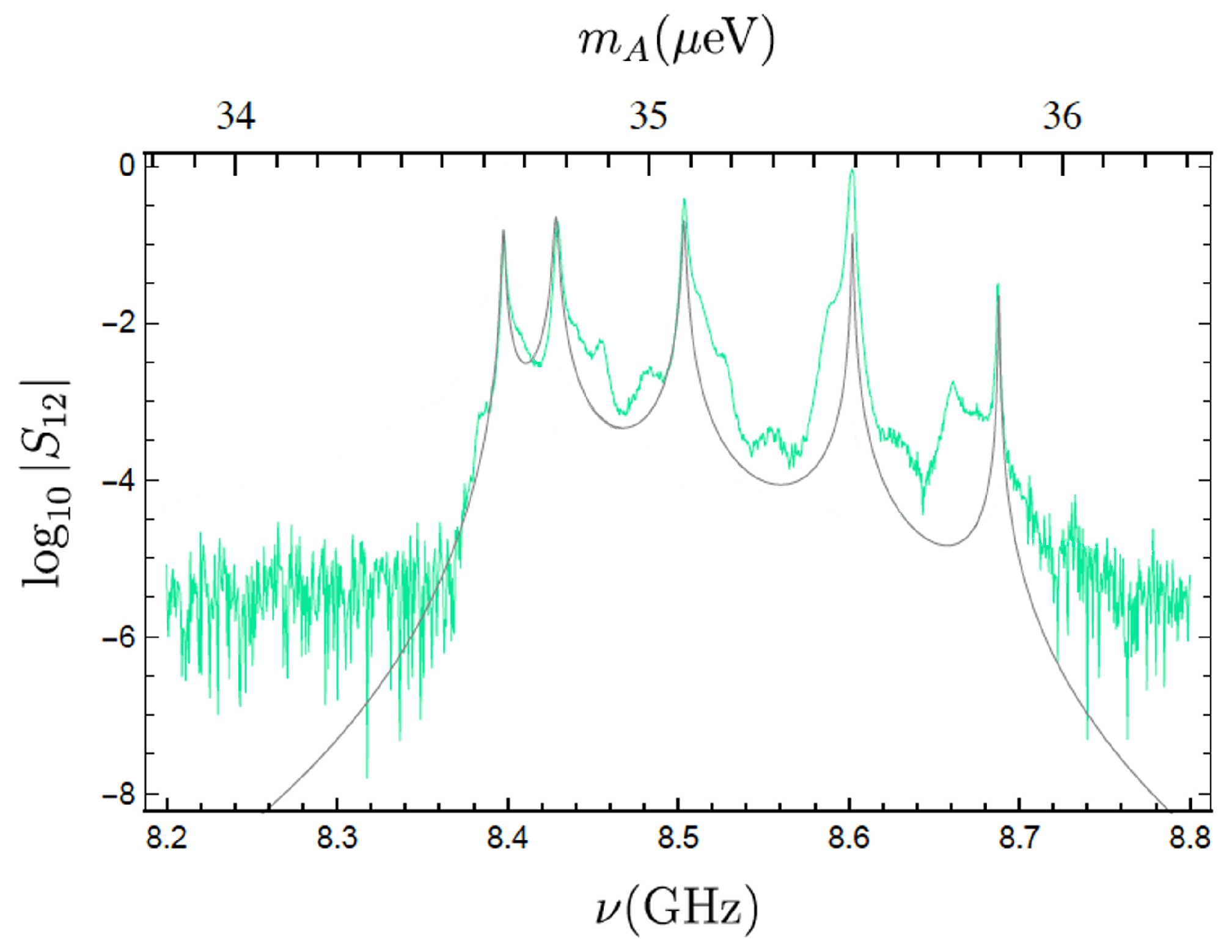
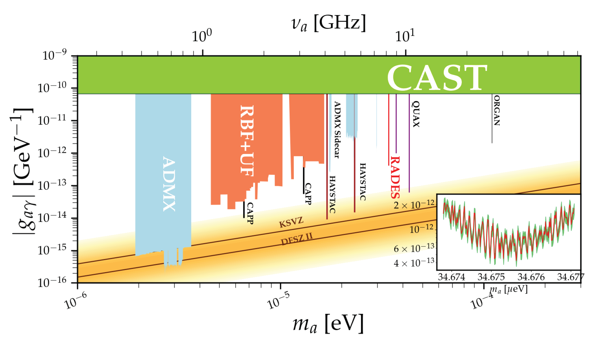
- Melcón, A.Á.; Arguedas Cuendis, S.; Baier, J.; Barth, K.; Bräuniger, H.; Calatroni, S.; Cantatore, G.; Caspers, F.; Castel, J.F.; Cetin, S.A.; et al. First results of the CAST-RADES haloscope search for axions at 34.67 μeV. J. High Energy Phys. 2021, 75. [Google Scholar]
- Keysight Technologies Application Note 5952-3706E 2019. Available online: www.keysight.com/es/en/assets/7018-06829/application-notes/5952-3706.pdf (accessed on 22 December 2021).
- Golm, J.; Arguedas Cuendis, S.; Calatroni, S.; Cogollos, C.; Döbrich, B.; Gallego, J.D.; García Barceló, J.M.; Granados, X.; Gutierrez, J.; Irastorza, I.G.; et al. Thin Film (High Temperature) Superconducting Radiofrequency Cavities for the search of axion dark matter. arXiv 2021, arXiv:2110.01296. [Google Scholar]
- The IAXO Collaboration; Abeln, A.; Altenmüller, K.; Arguedas Cuendis, S.; Armengaud, E.; Attié, D.; Aune, S.; Basso, S.; Bergé, L.; Biasuzzi, B.; et al. Conceptual design of BabyIAXO, the intermediate stage towards the International Axion Observatory. J. High Energy Phys. 2021, 137, 1–80. [Google Scholar]
- Dafni, T.; Galán, J. Digging into axion physics with (Baby)IAXO (submitted to Universe, Special Issue: Studying the Universe from Spain. In review process). arXiv 2021, arXiv:2112.02286. [Google Scholar]
- Arcioni, P.; Bressan, M.; Perregrini, L. A New Boundary Integral Approach to the Determination of Resonant Modes of Arbitrarily Shaped Cavities. IEEE Trans. Microw. Theory Tech. 1995, 43, 1848–1856. [Google Scholar] [CrossRef]
- Conciauro, G.; Guglielmi, M.; Sorrentino, R. Advanced Modal Analysis. CAD Techniques for Waveguide Components and Filters; John Wiley and Sons, Ltd.: Hoboken, NJ, USA, 2000. [Google Scholar]


| Dimensions (mm) | K | K |
|---|---|---|
| Cavity width (a) | 22.86 | 22.99 |
| Cavity height (b) | 10.16 | 10.25 |
| Length external cavities () | 26.68 | 26.82 |
| Length internal cavities () | 25.00 | 25.14 |
| Iris width () | 8.00 | 8.14 |
| Iris thickness (t) | 2.00 | 1.95 |
| Parameter | Value |
|---|---|
| 4577 Hz | |
| (7.8 ± 2.0) K | |
| 11,009 ± 483 | |
| 0.33 ± 0.05 | |
| (8.8 ± 0.0088) T | |
| 0.45 GeVcm−3 | |
| C | 0.65 |
| Volume | 0.03 l |
| 0.83 |
Publisher’s Note: MDPI stays neutral with regard to jurisdictional claims in published maps and institutional affiliations. |
© 2021 by the authors. Licensee MDPI, Basel, Switzerland. This article is an open access article distributed under the terms and conditions of the Creative Commons Attribution (CC BY) license (https://creativecommons.org/licenses/by/4.0/).
Share and Cite
Díaz-Morcillo, A.; García Barceló, J.M.; Lozano Guerrero, A.J.; Navarro, P.; Gimeno, B.; Arguedas Cuendis, S.; Álvarez Melcón, A.; Cogollos, C.; Calatroni, S.; Döbrich, B.; et al. Design of New Resonant Haloscopes in the Search for the Dark Matter Axion: A Review of the First Steps in the RADES Collaboration. Universe 2022, 8, 5. https://doi.org/10.3390/universe8010005
Díaz-Morcillo A, García Barceló JM, Lozano Guerrero AJ, Navarro P, Gimeno B, Arguedas Cuendis S, Álvarez Melcón A, Cogollos C, Calatroni S, Döbrich B, et al. Design of New Resonant Haloscopes in the Search for the Dark Matter Axion: A Review of the First Steps in the RADES Collaboration. Universe. 2022; 8(1):5. https://doi.org/10.3390/universe8010005
Chicago/Turabian StyleDíaz-Morcillo, Alejandro, José María García Barceló, Antonio José Lozano Guerrero, Pablo Navarro, Benito Gimeno, Sergio Arguedas Cuendis, Alejandro Álvarez Melcón, Cristian Cogollos, Sergio Calatroni, Babette Döbrich, and et al. 2022. "Design of New Resonant Haloscopes in the Search for the Dark Matter Axion: A Review of the First Steps in the RADES Collaboration" Universe 8, no. 1: 5. https://doi.org/10.3390/universe8010005
APA StyleDíaz-Morcillo, A., García Barceló, J. M., Lozano Guerrero, A. J., Navarro, P., Gimeno, B., Arguedas Cuendis, S., Álvarez Melcón, A., Cogollos, C., Calatroni, S., Döbrich, B., Gallego-Puyol, J. D., Golm, J., Irastorza, I. G., Malbrunot, C., Miralda-Escudé, J., Peña Garay, C., Redondo, J., & Wuensch, W. (2022). Design of New Resonant Haloscopes in the Search for the Dark Matter Axion: A Review of the First Steps in the RADES Collaboration. Universe, 8(1), 5. https://doi.org/10.3390/universe8010005