Scalar Perturbations of Black Holes in the $\mathit{f}\mathbf{\left(}\mathit{R}\mathbf{\right)}\mathbf{=}\mathit{R}\mathbf{-}\mathbf{2}\mathit{\alpha }\sqrt{\mathit{R}}$ Model

Abstract

In this paper, we study the perturbations of the charged static spherically symmetric black holes in the $f\left(R\right)=R-2\alpha \sqrt{R}$ model by a scalar field. We analyze the quasinormal modes spectrum, superradiant modes, and superradiant instability of the black holes. The frequency of the quasinormal modes is calculated in the frequency domain by the third-order WKB method, and in the time domain by the finite difference method. The results by the two methods are consistent and show that the black hole stabilizes quicker for larger $\alpha$ satisfying the horizon condition. We then analyze the superradiant modes when the massive charged scalar field is scattered by the black hole. The frequency of the superradiant wave satisfies $\omega \in (\frac{\mu }{\sqrt{2}},{\omega }_c)$, where $\mu$ is the mass of the scalar field, and ${\omega }_c$ is the critical frequency of the superradiance. The amplification factor is also calculated by numerical method. Furthermore, the superradiant instability of the black hole is studied analytically, and the results show that there is no superradiant instability for such a system.

1. Introduction

The problems of dark energy (DE) and dark matter (DM) have existed for a long time, for which there are no widely recognized causes till now. The most plausible explanation of DE and DM should be rooted in the quantum gravity. The first step towards quantum gravity is to address the shortcomings at ultraviolet and infrared [1] of the standard Einstein general relativity (GR). Then, it may be a natural consideration to extend the Lagrangian R of gravity to a more general form $f\left(R\right)$. This $f\left(R\right)$ modified gravity may give some phenomenological explanations of early or later universe. For example, the $f\left(R\right)=R+\alpha R^2(\alpha >0)$ model explains the inflationary behavior of the early universe successfully [2,3,4]. $f\left(R\right)=R-\frac{\beta }{R^n}$ model, where both $\beta$ and n are positive numbers, is able to explain the observed cosmic acceleration without assuming the cosmological constant [5,6,7]. Furthermore, more viable $f\left(R\right)$ models, which could describe the inflation, act as dark energy as well as passing the solar system tests, can be found in [8,9,10]. For more information of $f\left(R\right)$ gravity, one can see reviews [11,12].

Searching for static spherically symmetric (SSS) solutions is always of basic importance in any gravitational theory. SSS solutions in $f\left(R\right)$ gravity have also been widely discussed. The introducing of the nonlinear terms $R^n$ to the Lagrangian may lead to more mathematical difficulties and more possible solutions in the $f\left(R\right)$ model. The Birkhoff theorem is no longer valid for general $f\left(R\right)$ theories. Multamäki and Vilja found SSS solutions when the Ricci scalar is a constant [13,14]. Via the Noether symmetry approach, Capozziello etc. derived specific spherically symmetric solutions [15] as well as axially symmetric solutions [16]. Hollenstein and Lobo analyzed SSS solutions in $f\left(R\right)$ gravity coupled to nonlinear electrodynamics [17].

Among various $f\left(R\right)$ models, a specific model $f\left(R\right)=R-2\alpha \sqrt{R}$ is of special interest and attracts continuous attention, especially in searching for SSS solutions of the field equations in this and other similar models [13,18,19,20,21,22,23,24,25,26]. The parameter $\alpha$, which has the dimension of the inverse mass, is a key characteristic of this model, and thus plays a decisive role in constructing black holes (BHs). Charged SSS BH solutions in such a particular class of $f\left(R\right)$ models are obtained in [23]:

$$\begin{array}{cc}\hfill & d{s}^2=h\left(r\right)d{t}^2-h^{-1}\left(r\right)d{r}^2-r^{2}d{\Omega }^2,\hfill \\ & h\left(r\right)=\frac{1}{2}-\frac{1}{3\alpha r}+\frac{Q^2}{r^2},\hfill \end{array}$$

(1)

where the parameter $\alpha$ contributes to the mass of the BH as $M=\frac{1}{6\alpha }$, and Q is the electric charge that is independent of $\alpha$. The horizons of the BHs are located at

$$\begin{array}{cc}\hfill & r_{+}=2M+\sqrt{4M^2-2Q^2}=\frac{1}{3\alpha }(1+\sqrt{1-18{\alpha }^2{Q}^2}),\hfill \\ & r_{-}=2M-\sqrt{4M^2-2Q^2}=\frac{1}{3\alpha }(1-\sqrt{1-18{\alpha }^2{Q}^2}).\hfill \end{array}$$

(2)

Thus, the parameters have to satisfy the relation

$$0<\alpha \le \frac{1}{3\sqrt{2}Q}.$$

(3)

Obviously, the parameter $\alpha$ cannot be set to zero, thus these are new BH solutions constructed in the special class of $f\left(R\right)$ gravities, and cannot possibly be reduced to GR ones. These BHs are asymptotically flat but with a dynamical Ricci scalar $R=\frac{1}{r^2}$. In a successive paper [24], the author further proved that this is the unique SSS solution with $g_{tt}=-\frac{1}{g_{rr}}$ that deviates from GR and asymptotes as a flat spacetime for $f\left(R\right)=R-2\alpha \sqrt{R}$ model. After obtaining the BH solutions [23,24], the authors calculated some thermodynamic quantities versus the model parameter $\alpha$, including the entropy, quasi-local energy, Gibbs free energy, and the Hawking temperature, etc., and providing a detailed description of the physical properties including the stability and causal structure. Through these explorations, the authors tried to show that these BH solutions are physically acceptable.

We concern in this paper about the BH perturbation by the massive charged scalar fields (MCSFs). The BH perturbation theory dates back to 1957 by Regge and Wheele [27]. Soon after, the special modes of perturbation with purely outgoing waves at spatial infinity and ingoing waves near the horizon were identified by Vishveshwara [28] and named as quasinormal modes (QNMs) by Press [29]. After decades of research, several semi-analytical and numerical methods are widely used to calculate QNMs, in which the most popular methods are the WKB method [30,31,32,33,34] in frequency domain and the finite difference method [35,36] in time domain. The frequencies ${\omega }_n$ of QNMs are only allowed to be a series of complex values. The imaginary part indicates the evolution of the perturbation amplitude whose growth in time means the dynamical instability of the corresponding modes. Therefore, QNMs have become the essential aspects in the study of the stability of BHs [37,38].

In addition, superradiance [39] is an interesting phenomenon, which may extract energy from BHs. It is described by the perturbation of Boson fields scattered by BHs with both ingoing and outgoing waves existing at spatial infinity. When the energy of outgoing waves is larger than the energy of ingoing waves, superradiant scattering happens. Recent studies on superradiance in Reissner–Nordström (RN) spacetimes can be found in [40,41]. Moreover, to make superradiance a physical process, the laws of BH should be satisfied [42].

Provided there is an additional mechanism that can make the superradiant wave reflect back to the BH, superradiant modes will keep extracting energy from the central BH. Then, the total extracted energy may grow exponentially with time, for which Press and Teukolsky suggested an explosive phenomenon as an end state, dubbed the black hole bomb [43]. The nonnegligible backreaction on the background destabilizes the central black hole eventually, which is the superradiant instability of BHs [44]. A natural mechanism that can produce the superradiant instability is to introduce a mass term for boson fields [45,46,47,48,49]. However, Hod proved that the system of RN BHs and MCSFs has no superradiant instability [50,51,52]. This is because the two conditions, (i) the superradiant amplification of the boson field, and (ii) the existence of a binding potential well which can reflect the boson field back to the black hole, cannot operate simultaneously. In order to obtain superradiant instability in the non-rotating spacetime, Degollado et al. introduced a mirror-like boundary condition [53]. Soon after, Dolan et al. suggested that the endpoint of superradiant instabilities in RN spacetime is a hairy BH [54]. After that, Sanchis-Gual et al. did numerical relativity calculations [55,56] to simulate the hair growth process by superradiant instability of RN BHs in a cavity.

In this paper, we discuss three types of perturbation problems for BHs (1), including QNMs, superradiant scattering, and superradiant instability. We use two different methods to calculate the frequency of QNMs. In frequency domain, we adopt the third order WKB method to do the computation. Meanwhile, we use the finite difference method to evaluate the Klein–Gordon equation and use the Prony method to extract the main frequency in the time domain profiles. The results given by the two different methods are consistent, which show that the BH (1) is stable. Supperradiance is also discussed in spacetime (1).

This paper is organized as follows: In Section 2, we derive the radial equation satisfied by the perturbation theory of BHs (1). In Section 3, we separately calculate the frequencies of QNMs in frequency domain and in time domain. The third WKB method is used in frequency domain. In addition, we use the finite difference method to evaluate the Klein–Gordon equation outside the BH. Then, we use the Prony method to extract the main frequency. In Section 4, we analyze the frequency condition of supperradiant scattering, and compute the amplification factor. In Section 5, we analytically study the extreme points of the effective potential, and prove there is no superradiant instability for the system of BHs (1) and MCSFs. In Section 6, we discuss the deficit angle of BHs (1) and use a physical method to obtain the frequency condition of superradiance. Finally, we give a conclusion in Section 7. In this paper, we adopt the units $G=\hslash =c=1$.

2. The Klein–Gordon Equation

We discuss the perturbation problems of BH (1) by MCSFs. Assume there is a massive charged scalar field $\Phi$ in spacetime (1) and the energy-momentum tensor of the scalar field is small enough so that it cannot affect the background spacetime. Thus, the evolution of the scalar field is described by Klein–Gordon equation

$$[({\nabla }_{\nu }-iq{A}_{\nu })({\nabla }^{\nu }-iq{A}^{\nu })-{\mu }^2]\Phi =0,$$

(4)

where $A_{\nu }=(-\frac{Q}{r},0,0,0)$ is the electromagnetic potential, q is the charge, and $\mu$ is the mass of the scalar field. In the frequency domain, the scalar field can be separated in spherical coordinate by

$$\Phi (t,r,\theta ,\phi )=\sum _{l,m}{e}^{-i\omega t}{Y}_{lm}(\theta ,\phi )\frac{{\psi }_l\left(r\right)}{r},$$

(5)

where $Y_{lm}(\theta ,\phi )$ is the spherical harmonics. Plugging the metric (1) into the evolution Equation (4), we obtain the radial equation

$$h^2{\psi }_l^{″}+h{h}^{\prime }{\psi }_l^{\prime }+[{(\omega -\frac{qQ}{r})}^2-h(\frac{h^{\prime }}{r}+\frac{l(l+1)}{r^2}+{\mu }^2)]{\psi }_l=0.$$

(6)

By using the tortoise coordinate $dx=\frac{dr}{h\left(r\right)}$, we can reduce the radial equation to Schrödinger-like form

$$\frac{d^2}{d{x}^2}{\psi }_l\left(r\right)+[{(\omega -\frac{qQ}{r})}^2-V\left(r\right)]{\psi }_l\left(r\right)=0,$$

(7)

where

$$V\left(r\right)=h\left(r\right)(\frac{h^{\prime }\left(r\right)}{r}+\frac{l(l+1)}{r^2}+{\mu }^2)$$

(8)

is the effective potential. Note that the interaction term $\frac{qQ}{r}$ is coupled with $\omega$ and not included in $V\left(r\right)$. Equation (7) is the main equation that the perturbation theory satisfies. The perturbation theory can be used to study QNMs, absorption and scattering problem, supperadiant instability, etc. Each problem has its own boundary conditions. In the following numerical investigations, we only list the results for the typical modes of $n=0$ and $l=2$.

3. QNMs

For simplicity, we investigate the QNMs under the perturbation of a neutral massless scalar field $\mu =0,q=0$. Since the waves at spatial infinity are purely outgoing and those near the horizon are purely ingoing, the boundary conditions of QNMs are taken as

$${\psi }_l=\left\{\begin{array}{cc}{e}^{-i\omega x},\hfill & x\to -\infty ;\hfill \\ e^{i\omega x},\hfill & x\to \infty .\hfill \end{array}\right.$$

(9)

The frequencies $\omega ={\omega }_{nl}$ are the eigenvalues of Equation (6) with conditions (9). In the following, we will use two different methods to calculate the frequencies and compare the results.

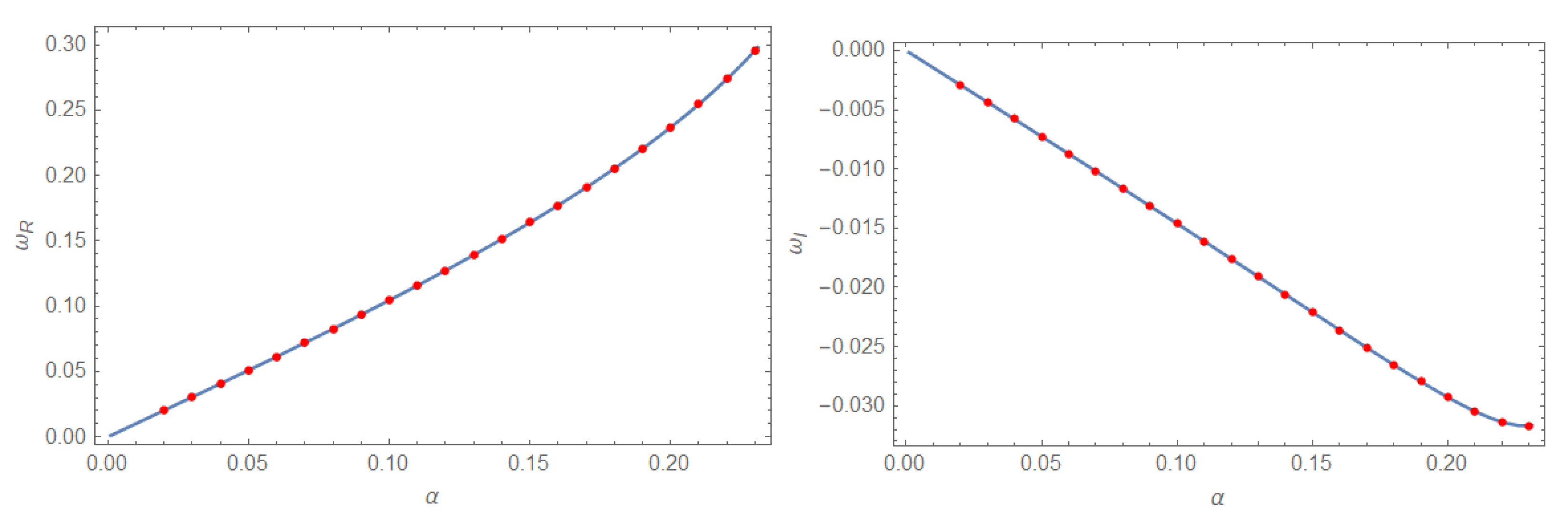
3.1. Frequency Domain

We use the third order WKB method to calculate the eigenfrequencies ${\omega }_{nl}$. The WKB method is an approximate method to solve linear differential equations, especially the time-dependent Schrödinger equation. As we have shown, the radial equation of perturbation theory is a Schrödinger-like form (7). Due to this similarity, Schutz and Will [30] first introduced the WKB method to calculate the eigenfrequencies of QNMs. On this basis, Iyer and Will [31] established the third order approximation method. Soon after, Konoplya [34] extended it to the sixth order. In this paper, we use the third order method. To use the WKB method, we have to consider the perturbation of a neutral scalar field. In this case, the influence of the term $\frac{qQ}{r}$ in Equation (7) vanishes. Following [57], we have

$${\omega }^2=(V+\sqrt{-2V^{\left(2\right)}}\Gamma )-i(1+\Omega )\sqrt{-2V^{\left(2\right)}\Xi },$$

(10)

where

$$\begin{array}{cc}\hfill \Xi =& {(n+\frac{1}{2})}^2,\hfill \\ \hfill \Gamma =& \frac{1}{\sqrt{-2V^{\left(2\right)}}}\left[\frac{1}{8}\left(\frac{V^{\left(4\right)}}{V^{\left(2\right)}}\right)\left(\frac{1}{4}+\Xi \right)-\frac{1}{288}{\left(\frac{V^{\left(3\right)}}{V^{\left(2\right)}}\right)}^2\left(7+60\Xi \right)\right],\hfill \\ \hfill \Omega =& -\frac{1}{2V^{\left(2\right)}}[\frac{5}{6912}{\left(\frac{V^{\left(3\right)}}{V^{\left(2\right)}}\right)}^4(77+188\Xi )-\frac{1}{384}\left(\frac{{\left(V^{\left(3\right)}\right)}^2{V}^{\left(4\right)}}{{\left(V^{\left(2\right)}\right)}^3}\right)(51+100\Xi )\hfill \\ \hfill & +\frac{1}{2304}{\left(\frac{V^{\left(4\right)}}{V^{\left(2\right)}}\right)}^2(67+68\Xi )+\frac{1}{288}\left(\frac{V^{\left(3\right)}{V}^{\left(5\right)}}{{\left(V^{\left(2\right)}\right)}^2}\right)(19+28\Xi )-\frac{1}{288}\left(\frac{V^{\left(6\right)}}{V^{\left(2\right)}}\right)(5+4\Xi )].\hfill \end{array}$$

The derivatives of the potential $V^{\left(n\right)}$ are defined by

$$V^{\left(n\right)}=\frac{d^{n}V}{d{x}^n}=h\left(r\right)\frac{d}{dr}{V}^{(n-1)}.$$

(11)

The coordinates of Equation (10) locate in the maximum point of the effective potential V.

The numerical results are presented in

Table 1. The eigenfrequencies of QNMs for different values of the parameters $\alpha$ and Q.

$\mathit{\alpha }$	Q = 0	Q = 0.5	Q = 1
0.05	0.0506405–0.00723841i	0.0507361–0.00724286i	0.0510277–0.00725603i
0.10	0.101281–0.0144768i	0.102055–0.0145121i	0.104545–0.0146107i
0.15	0.151921–0.0217152i	0.154592–0.0218319i	0.164079–0.0220981i
0.20	0.202562–0.0289536i	0.209090–0.0292214i	0.236908–0.0292890i
0.25	0.253202–0.0361920i	0.266504–0.0366856i
0.30	0.303843–0.0434305i	0.328158–0.0441963i
0.35	0.354483–0.0506689i	0.396082–0.0516327i
0.40	0.405124–0.0579073i	0.473815–0.0585780i
0.45	0.455764–0.0651457i	0.568936–0.0632737i
0.50	0.506405–0.0723841i

and Figure 1. The real part of the eigenfrequencies represents the oscillation of the scalar field, while the imaginary part indicates the evolution of the perturbation amplitude. The positive value of the imaginary part means the growth of the perturbation amplitude and hence the dynamical instability of the corresponding modes, while negative value means decay and hence stability. Table 1 shows the eigenfrequencies for different values of the parameters $\alpha$ and Q constrained by Equation (3). As is shown in Table 1, the imaginary part of all eigenfrequencies are negative, which means BHs (1) are stable. Moreover, one can see from Figure 1 that the imaginary part becomes more negative with $\alpha$ increasing. That is to say, BHs with larger $\alpha$ stabilize quicker. In contrast, the imaginary part of the eigenfrequencies is insensitive to the values of Q, which is easy to see from Table 1 and Figure 1.

3.2. Time Domain

In the time domain, we numerically solve the Klein–Gordon Equation (4) without implying the stationary ansatz $\Phi =e^{-i\omega t}$. Plugging $\Phi =\frac{\chi (r,t)}{r}{Y}_{lm}(\theta ,\phi )$ into (4), we obtain the equation

$$\frac{{\partial }^2\chi (x,t)}{\partial x^2}-\frac{{\partial }^2\chi (x,t)}{\partial t^2}-V\left(x\right)\chi (x,t)=0.$$

(12)

Note that we use the coordinate x to replace the radial coordinate r. In general, we cannot find an analytical form for the function $r\left(x\right)$. However, it is possible to find a numerical list between r and x. Using the light-cone coordinates $\tilde{u}=t-x$, $\tilde{v}=t+x$, we rewrite Equation (12) as

$$[4\frac{{\partial }^2}{\partial \tilde{u}\partial \tilde{v}}+V(\tilde{u},\tilde{v})]\chi (\tilde{u},\tilde{v})=0.$$

(13)

We numerically integrate Equation (13) on a $\tilde{u},\tilde{v}$ null grid [35,36]. Note that the properties of QNMs are independent of the initial conditions. For simplicity, we choose the initial condition as

$$\chi (\tilde{u},0)=0,\chi (0,\tilde{v})=1.$$

(14)

The numerical calculations are performed in a selected area and are shown in Figure 2. The left panel is the results for different $\alpha$ and the right is for different Q. One can see that the scalar field decays quicker for larger $\alpha$. That is to say, the BHs with larger $\alpha$ stabilizes quicker, which is a consistent behavior with the WKB method. In addition, the insensitivity of the decay of the scalar field to the parameter Q is also confirmed here.

In order to extract the quasinormal frequency in time domain profile, we use the Prony method of fitting the profile data [58]. As an example, we obtain the frequency $\omega =0.104569-0.0146088i$ in the case $\alpha =0.10, Q=1$. The corresponding result given by the WKB method is $\omega =0.104545-0.0146107i$, which shows an error less than one thousandth. More generally, we plot Figure 3 to compare the results given by the WKB method and by time domain profiles, which shows well consistent behaviors between the two methods.

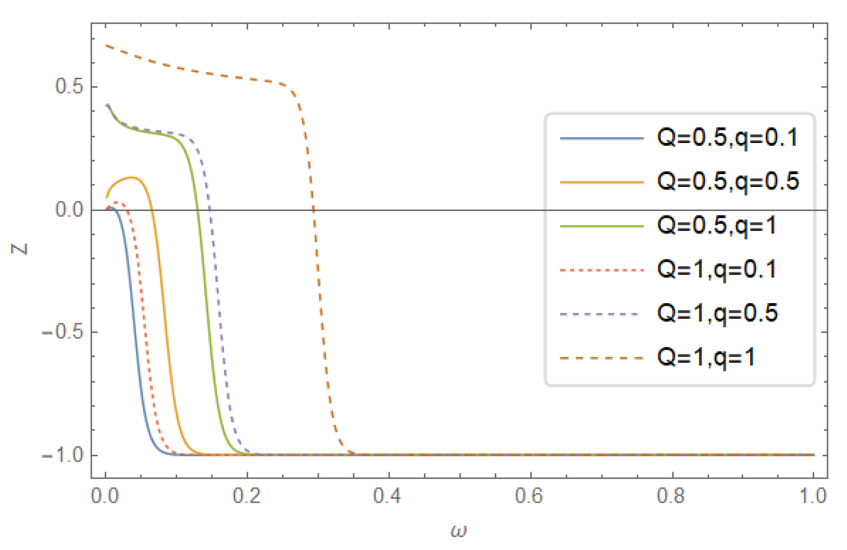
4. Superradiant Scattering

In order to obtain the superradiant modes, the perturbation field should be massive (massless) and charged. The solutions approaching the boundaries can be obtained from Equation (7):

$${\psi }_l\approx \left\{\begin{array}{cc}{e}^{-i\omega vr}+R_l{e}^{i\omega vr},\hfill & \mathrm{for}r\to \infty ;\hfill \\ T_l{e}^{-i\omega \xi x},\hfill & \mathrm{for}r\to r_{+}.\hfill \end{array}\right.$$

(15)

where $|R_l{|}^2$ is the reflection coefficient, $|T_{\omega l}{|}^2$ is the transmission coefficient, $v=\sqrt{1-\frac{{\mu }^2}{2{\omega }^2}}$ is the speed of propagation of the wave in the far field, and $\xi =1-\frac{{\omega }_c}{\omega }$. The conservation of flux indicates a relationship between the reflection coefficient and the transmission coefficient

$$|R_l{|}^2+\frac{\xi }{v}{\left|T_l\right|}^2=1.$$

(16)

If $\xi >0$, $e^{-i\omega \xi x}$ is an ingoing wave and the BH absorbs the wave. However, if $\xi <0$, instead of an ingoing wave, we obtain an outgoing wave $e^{-i\omega \xi x}$ on the horizon. In addition, in this case, the reflection coefficient $|R_l{|}^2$ is larger than 1 because this outgoing wave reinforces the emergent wave at infinity. The energy of the BH is also extracted by scattering wave to infinity. Therefore, the superradiance only occurs when $\frac{\mu }{\sqrt{2}}<\omega <{\omega }_c$. We emphasize that this condition only corresponds to the scattering problem outside the BHs.

The amplification factor Z is defined by

$$Z=\frac{|R_l{|}^2}{|T_l{|}^2}-1.$$

(17)

When superradiance occurs, the amplification factor Z should be positive since the reflection coefficient $|R_l{|}^2$ is larger than the transmission coefficient $|T_l{|}^2$. The amplification factor Z is also used to indicate the intensity of superradiance.

We solve numerically the radial Equation (6) with boundary conditions (15). The solutions are expanded near both the horizon and the infinity. The corresponding boundary conditions are taken to be the first order expansion. Using the asymptotical expressions given by Equation (15) and its derivatives, we numerically integrate the radial Equation (6) from somewhere adjacent to the event horizon to somewhere far away. Then, by matching the numerical integration and the expansion of solution approaching infinity, we obtain the reflection and transmission coefficients. Furthermore, we calculate the amplification factor Z and show the numerical results in Figure 4.

The superradiance modes exist in the range $Z>0$, which is shown in Figure 4. The critical frequency ${\omega }_c$ is located at $Z\left({\omega }_c\right)=0$. It is easy to see that, when $\omega <{\omega }_c$, we have $Z>0$. Since the horizon $r_{+}$ decreases as parameter Q increases, the critical frequency ${\omega }_c=\frac{qQ}{r_{+}}$ increases as parameter Q increases, which is clearly shown in Figure 4. The monotonous increase of ${\omega }_c$ with q is obvious.

If the superradiance scattering modes can be detected, there must be an appropriate frequency window satisfying $\frac{\mu }{\sqrt{2}}<\omega <{\omega }_c$, which means that the ratios $\eta =\frac{Q}{M}$ and $\frac{\mu }{q}$ must satisfy

$$\frac{\mu }{q}<\frac{\eta }{\sqrt{2}+\sqrt{2-{\eta }^2}}.$$

(18)

We plot the parameter space of $(\eta ,\frac{\mu }{q})$ in Figure 5. The line satisfies ${\omega }_c=\frac{\mu }{\sqrt{2}}$. Above this line, superradiant scattering is forbidden.

5. Superradiant Instability

The superradiance can also exist in a bound state system provided there is an additional mechanism that can restrain the superradiant field around the BH. In this case, superradiant modes will keep extracting energy from the central BH and destabilize the background spacetime eventually. A natural mechanism is to introduce a mass term into the boson field that offers an attractive force between the central BH and the massive field. In the case of rotating charged BHs, the MCSFs may lead to the superradiant instabilities. However, such a mechanism cannot make the RN black hole unstable. Hod has shown that the system of the RN BHs and MCSFs is always stable [50]. In order to obtain the bound state, the effect potential should have a minimum so that the potential well can bound the superradiant modes. However, for the system of RN BHs and MCSFs, there is only one maximum point for the effect potential outside the horizon. That is to say, the superradiant modes cannot form bound state. Following his work, we analyze all of the four extreme points of the effective potential and show that only one maximum point is in the physical regime. Thus, the superradiant instability of the BHs (1) and MCSFs system cannot be triggered.

We still consider the radial Equation (7). Now, the boundary condition is chosen to be

$$\psi \sim \left\{\begin{array}{cc}{e}^{-i(\omega -{\omega }_c)x},\hfill & x\to -\infty ;\hfill \\ e^{-\sqrt{\frac{{\mu }^2}{2}-{\omega }^2}x},\hfill & x\to \infty .\hfill \end{array}\right.$$

(19)

Defining a new radial function $\varphi$,

$$\varphi =h{\left(r\right)}^{\frac{1}{2}}\psi ,$$

(20)

we rewrite Equation (7) as

$$\frac{d^2\varphi }{d{r}^2}+({\omega }^2-U)\varphi =0,$$

(21)

where

$$U={\omega }^2-\frac{1}{\Delta }(\frac{2M}{r}-\frac{2Q^2}{r^2})-\frac{({(\omega -\frac{qQ}{r})}^2-V)r^4+M^2-\frac{Q^2}{2}}{{\Delta }^2}$$

(22)

with

$$\Delta =\frac{r^2}{2}-2Mr+Q^2.$$

(23)

If it is not limited to the scattering problem, the superradiant condition becomes $\omega <{\omega }_c$. In addition, the binding potential well satisfies $\omega <\frac{\mu }{\sqrt{2}}$. Therefore, the overlapping region between the superradiant condition and the bound state condition implies

$$0<\omega <min\{{\omega }_c,\frac{\mu }{\sqrt{2}}\}.$$

(24)

Then, the important task is to analyze the behavior of the effective potential U.

Following [50,51,52], we define

$$z=r-r_{-}.$$

(25)

The derivative of the effective potential $U^{\prime }=\frac{dU}{dr}$ satisfies

$$-\frac{{\Delta }^3}{2}{U}^{\prime }(r;M,Q,\mu ,q,\omega ,l)=a{z}^4+b{z}^3+c{z}^2+dz+e,$$

(26)

where the coefficients $a,b,c,d,e$ are given by

$$\begin{array}{cc}\hfill a& =-2M{\omega }^2+\frac{1}{2}qQ\omega +\frac{1}{2}M{\mu }^2,\hfill \end{array}$$

(27)

$$\begin{array}{cc}\hfill b& =(2M{r}_{-}-2M^2-\frac{1}{2}{Q}^2){\mu }^2+(-8M{r}_{-}+2Q^2){\omega }^2+2(M+r_{-})qQ\omega -\frac{1}{2}{q}^2{Q}^2\hfill \\ & +\frac{1}{4}l(l+1),\hfill \end{array}$$

(28)

$$\begin{array}{cc}\hfill c& =-\frac{3}{8}{r}_{-}^2(r_{+}-r_{-}){\mu }^2+3r_{-}^3(\frac{qQ}{r_{-}}-\omega )(\omega -\frac{qQ}{2r_{-}})-\frac{3}{4}l(l+1)(2M-r_{-}),\hfill \end{array}$$

(29)

$$\begin{array}{cc}\hfill d& =2{\omega }^2{Q}^2{r}_{-}^2-2{\omega }^2{r}_{-}^4+\frac{7}{2}qQ\omega r_{-}^3-\frac{1}{2}{Q}^2{\mu }^2{r}_{-}^2+\frac{1}{8}{\mu }^2{r}_{-}^4+\frac{1}{2}{\mu }^2{Q}^4-3q{Q}^3\omega r_{-}\hfill \\ \hfill & +q^2{Q}^4-\frac{3}{2}{q}^2{Q}^2{r}_{-}^2-\frac{3}{4}M{r}_{-}+\frac{1}{2}l(l+1)(4M^2+Q^2)-\frac{3}{4}l(l+1)(4M{r}_{-}-r_{-}^2)\hfill \\ \hfill & +\frac{1}{2}(Q^2-M^2)+M^2-\frac{3}{8}M(r_{+}-r_{-}),\hfill \end{array}$$

(30)

$$\begin{array}{cc}\hfill e& =\frac{1}{2}{r}_{-}^4{(\omega -\frac{qQ}{r_{-}})}^2(r_{+}-r_{-})+\frac{1}{32}{(r_{+}-r_{-})}^3.\hfill \end{array}$$

(31)

It is easy to find the asymptotic behavior of $U^{\prime }$ as

$$U^{\prime }\left(r\right)=-\frac{16a}{r^2}+O(\frac{1}{r^3}).$$

(32)

We now analyze the roots $\left\{z_1,z_2,z_3,z_4\right\}$ of the quartic equation $U^{\prime }\left(z\right)=0$. There are well-known relations between them

$$\begin{array}{cc}\hfill z_1+z_2+z_3+z_4& =-\frac{b}{a},\hfill \end{array}$$

(33)

$$\begin{array}{cc}\hfill z_1{z}_2+z_1{z}_3+z_1{z}_4+z_2{z}_3+z_2{z}_4+z_3{z}_4& =\frac{c}{a},\hfill \end{array}$$

(34)

$$\begin{array}{cc}\hfill z_1{z}_2{z}_3+z_1{z}_2{z}_4+z_1{z}_3{z}_4+z_2{z}_3{z}_4& =-\frac{d}{a},\hfill \end{array}$$

(35)

$$\begin{array}{cc}\hfill z_1{z}_2{z}_3{z}_4& =\frac{e}{a}.\hfill \end{array}$$

(36)

The coefficient a is always positive when $\omega$ is in the range (24). It is easy to prove this conclusion. We solve $a\left(\omega \right)=0$, and obtain the bigger root

$${\omega }_{+}=\frac{qQ+\sqrt{q^2{Q}^2+16M^2{\mu }^2}}{8M}.$$

(37)

If $\omega <\frac{qQ}{r_{+}}<\frac{\sqrt{2}}{2}\mu$, we use ${\omega }_{+}>\frac{qQ}{4r_{+}}+\sqrt{\frac{q^2{Q}^2}{16r_{+}^2}+\frac{q^2{Q}^2}{2r_{+}^2}}=\frac{qQ}{r_{+}}>\omega$; If $\omega <\frac{\sqrt{2}}{2}\mu <\frac{qQ}{r_{+}}$, we use ${\omega }_{+}>\frac{\sqrt{2}}{8}\mu +\sqrt{\frac{{\mu }^2}{32}+\frac{{\mu }^2}{4}}=\frac{\sqrt{2}}{2}\mu >\omega$. Thus, the conclusion $a>0$ is proved.

Then, from Equation (32), we know that

$$U^{\prime }(r\to \infty )\to 0^{-}.$$

(38)

Note also that

$$\begin{array}{cc}\hfill U(r\to r_{-})& ⟶-\infty ,\hfill \end{array}$$

(39)

$$\begin{array}{cc}\hfill U(r\to r_{+})& ⟶-\infty .\hfill \end{array}$$

(40)

Equations (38)–(40) imply that $U\left(r\right)$ has at least one maximum point in both the regions $(r_{+},\infty )$ and $(r_{-},r_{+})$. We arrange

$$0<z_2<r_{+}-r_{-}<z_1.$$

(41)

It is also easy to show $e>0$, and thus, from Equation (36), we have

$$z_1{z}_2{z}_3{z}_4>0,$$

(42)

which implies that $z_3,z_4$ must be both positive or both negative. In the following, we will analyze $z_3,z_4$ further.

If $c\le 0$, from Equaiton (34), we have

$$z_1{z}_2+z_1{z}_3+z_1{z}_4+z_2{z}_3+z_2{z}_4+z_3{z}_4\le 0,$$

(43)

which means that $z_3,z_4$ are both negative.

If $c>0$, from Equation (29), one can find that the necessary condition for $c>0$ is $(\frac{qQ}{r_{-}}-\omega )(\omega -\frac{qQ}{2r_{-}})>0$. Then, one obtains $\frac{qQ}{2r_{-}}<\omega <\frac{qQ}{r_{+}}$. Substituting Equation (2) into this inequality and solving it, we find in this case that the value of $\alpha$ must be taken in the range satisfying $\eta =\frac{Q}{M}<\frac{4}{3}$. Taking Equation (24) and using the inequality that $\frac{qQ}{2r_{-}}<\omega$, one realizes that the range of $\omega$ becomes

$$\frac{qQ}{2r_{-}}<\omega <min\left\{\frac{qQ}{r_{+}},\frac{\mu }{\sqrt{2}}\right\}.$$

(44)

Next, one can prove that $b>0$ when $c>0$. Then, from Equation (33), we have $z_1+z_2+z_3+z_4<0$, which means that $z_3,z_4$ are both negative. To prove $b>0$, one needs to prove that the minimum of b is positive. The two cases of positive and negative coefficient of ${\mu }^2$ in Equation (28) should be analyzed separately. The detailed analysis is primary and tedious, so we put the analysis process in Appendix A.

Through the analysis, one can prove that $z_3$, $z_4$ are both negative. This means that, among the four extreme points $\left\{z_1,z_2,z_3,z_4\right\}$ of the effective potential $U\left(r\right)$, only one maximum point $z_1$ is in the physical region, which shows that there is no binding potential well outside the black hole($r>r_{+}$). Therefore, we conclude that there is no superradiant instability for the system of BHs (1) and the MCSFs.

6. Further Discussion

6.1. Deficit Angle

BHs (1) are different from RN BHs in two aspects. First, the dimensional parameter $\alpha$ describes the mass M of the BHs. Secondly, BHs (1) have a fixed deficit angle $\delta \theta =\pi$. It is clear that through coordinate transformation $r=\frac{\rho }{\sqrt{2}}$ and $t=\sqrt{2}\tau$, BHs (1) can be reexpressed as

$$\begin{array}{cc}\hfill d{s}^2& =h\left(\rho \right)d{\tau }^2-h^{-1}\left(\rho \right)d{\rho }^2-{\rho }^2\left(1-\frac{\delta \theta }{2\pi }\right)d{\Omega }^2,\hfill \\ \hfill h\left(\rho \right)& =1-\frac{2\sqrt{2}}{3\alpha \rho }+\frac{4Q^2}{{\rho }^2}.\hfill \end{array}$$

(45)

We often encounter the deficit angle issue in the studies related to monopole, high dimensional theory and some modified BH solutions. The global monopole solutions have a very small deficit angle $\delta \theta =ϵ$ [59]. The deficit angle of extra dimensions can be used to explain the cosmological constant problem [60]. A modified BH solution with small deficit angle in Lorentz breaking massive gravity has also been obtained [61].

It is also convenient to use the line element (45) to explain or study the properties of BHs (1). For example, the radial Equation (6) of perturbation theory can be rewritten as

$$\begin{array}{cc}\hfill h^2{\psi }^{**}& +h{h}^{*}{\psi }^{*}+[{({\omega }^{\prime }-\frac{qQ}{\sqrt{2}\rho })}^2-V\left(\rho \right)]\psi =0,\hfill \\ \hfill V=& h\left(\frac{h^{*}}{\rho }+\frac{l(l+1)}{{\rho }^2(1-\frac{\delta \theta }{2\pi })}+{\mu }^2\right),\hfill \end{array}$$

(46)

where $h=h\left(\rho \right)$, and * and ** denote one and second order derivatives with respect to $\rho$, respectively. Since the time coordinate becomes $\tau$, the frequency ${\omega }^{\prime }$ of the wave described by radial Equation (46) and the frequency $\omega$ described by Equation (6) satisfy

$${\omega }^{\prime }=\sqrt{2}\omega .$$

(47)

It is easy to see that the deficit angle $\delta \theta$ only influences $\psi$ when $l\ne 0$. Furthermore, all the preceding results can be reproduced by solving the new radial Equation (46).

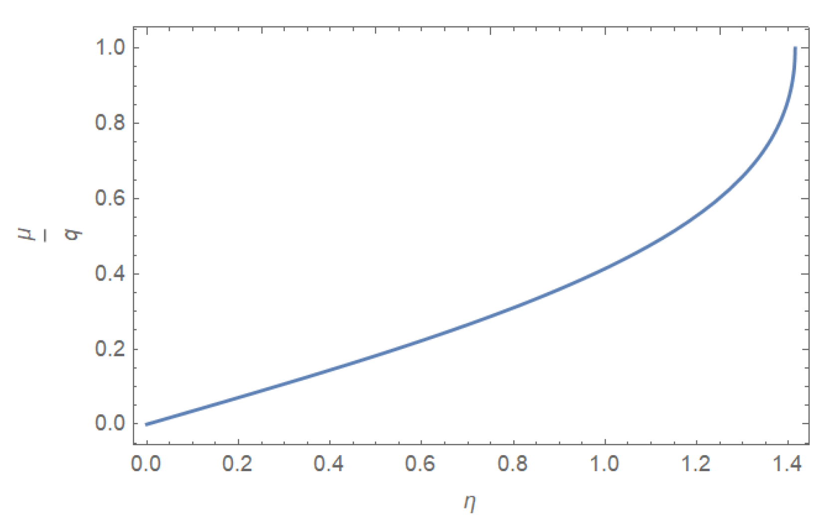
6.2. The Frequency Condition of Superradiance

The superradiance may exist both in the scattering state problem and bound state problem. In the previous discussion, we obtain the frequency condition of superradiance by analyzing the solution of radial equation. However, in the superradiance process, the bound condition near the horizon is an outgoing wave instead of an ingoing wave. It is known that BHs absorb everything naturally. Then, one may wonder whether the superradiance solution of radial equation can really happen in physics. The method introduced by Bekenstein [42] can answer this question. The idea is based on the area law of black hole, independent of detailed examination of the wave equation. Through this method, we will see the superradiance is not a mathematical solution but a real physical process. Following his work, we can also obtain the frequency condition of superradiance in a physical way.

The process of extracting energy from BHs must satisfy the Hawking’s theorem that the area of the BH can never decrease. The area of BHs (45) is $A=4\pi \left(1-\frac{\delta \theta }{2\pi }\right){\rho }_{+}^2$. The differential of the horizon area A is proportional to $dM-\tilde{\varphi }dQ$, where $\tilde{\varphi }=\frac{Q}{{\rho }_{+}}$. Far from the BH, the scattering wave may be regarded to be composed of many quanta (scalarons, mesons, electrons, etc.). The energy of each quantum is $\hslash \omega$ and the electric charge of each quantum is $\frac{q}{\hslash }$. The ratio of Coulomb energy to the energy carried by the wave must be $q/{\omega }^{\prime }$. On the other hand, the extraction of mass $dM$ is proportional to ${\omega }^{\prime }$ and the extraction of electric charge $dQ$ is proportional to q. However, the charge outside the event horizon becomes $\frac{Q}{\sqrt{2}}$. Thus, in the superradiance process, there must be $dQ=\frac{q}{\sqrt{2}{\omega }^{\prime }}dM$ from the conservation laws for energy and electric charge. Therefore, the change of area is expressed as

$$dA\propto (1-\frac{qQ}{\sqrt{2}{\rho }_{+}{\omega }^{\prime }})dM=(1-\frac{\sqrt{2}{\omega }_c}{{\omega }^{\prime }})dM.$$

(48)

If ${\omega }^{\prime }>\sqrt{2}{\omega }_c$, the mass of the BH increases, which means that the BH absorbs the wave. If ${\omega }^{\prime }<\sqrt{2}{\omega }_c$, the mass of the BH decreases, which means that the BH radiates the wave. We then conclude that the superradiance does happen physically and its frequency satisfies $\omega <{\omega }_c$.

7. Conclusions

The BH solutions given in Equation (1) are new charged SSS solutions obtained from the special class of $f\left(R\right)$ gravity. The model parameter $\alpha$ contributes to the mass of the BH and cannot be set to zero, which makes the BHs deviate from the standard solutions of GR. In this paper, we study the perturbation problem of BH (1) by MCSFs in three cases: QNMs, superradiant scattering, and superradiant instability. The three problems are described by the same radial Equation (7) but with different boundary conditions. The main conclusions are as follows:

(i) The third order WKB method is used to calculate QNMs in the frequency domain and the finite difference method is used in the time domain. The results indicate that the BH (1) is stable and stabilizes quicker with larger $\alpha$ constrained by the horizon condition Equation (3).

(ii) We analyze the superradiant scattering and obtain the condition of superradiant scattering $\frac{\mu }{\sqrt{2}}<\omega <{\omega }_c$. Since the metric function $h\left(r\right)$ is approximate to $\frac{1}{2}$ when $r\to \infty$, the effective potential $V\left(r\right)$ approaches $\frac{{\mu }^2}{2}$ when $r\to \infty$. Furthermore, the scattering modes approaching infinity satisfy $\omega >\frac{\mu }{\sqrt{2}}$, which is different from the frequency condition of scattering states in the RN metric. The amplification factor is calculated numerically. In some parameter region, there is no frequency window satisfying $\frac{\mu }{\sqrt{2}}<\omega <{\omega }_c$. Therefore, the superradiant scattering is forbidden above the line in Figure 5.

(iii) We prove that there is no superradiant instability for the system of BHs (1) and MCSFs. Through analyzing the extreme points of the potential, we show there is only one maximum point but no minimum one outside the BH. Thus, the conditions of superradiant amplification and binding potential well cannot be satisfied simultaneously.

(iv) We also show that the spacetime of BHs (1) has a fixed deficit angle $\delta \theta =\pi$. The previous conclusions can be reobtained by the metric (45) with deficit angle. Using this metric, we obtain the frequency condition of superradiance based on the Hawking’s theorem that the area of BHs never deceases. This method, independent of detailed examination of radial equation, would be more physical.

Our study indicates that the BHs (1) are stable under the perturbation of the scalar field. Possibly, it is just the deviation of these BHs from the ones in GR that attracts the continuous interest in recent years. However, a concomitant question may come: “Is it possible to have BHs with different values of mass in this special $f\left(R\right)=R-2\alpha \sqrt{R}$ model?” What is certain is there must be other BH solutions in this $f\left(R\right)$ model. Maybe there are some generic solutions that allow different values of the mass and include the solutions (1) as a special case. To have a clearer physical picture, further investigations are needed. Moreover, it is worth studying further about more astrophysical characteristics such as the formation and collapse of these BHs. Comparing the predictions from these BHs with those from GR and with the astrophysical observations would be very interesting and expected.

References

1. Capozziello, S.; Laurentis, M.D. Extended Theories of Gravity. Phys. Rept. 2011, 509, 167. [Google Scholar] [CrossRef] [Green Version]
2. Starobinsky, A.A. A New Type of Isotropic Cosmological Models without Singularity. Phys. Lett. B 1980, 91, 99. [Google Scholar] [CrossRef]
3. Nojiri, S.; Odintsov, S.D. Modified gravity with negative and positive powers of the curvature: Unification of the inflation and of the cosmic acceleration. Phys. Rev. D 2003, 68, 123512. [Google Scholar] [CrossRef] [Green Version]
4. Nojiri, S.; Odintsov, S.D. Modified gravity with ln R terms and cosmic acceleration. Gen. Rel. Grav. 2004, 36, 1765. [Google Scholar] [CrossRef] [Green Version]
5. Capozziello, S. Curvature Quintessence. Int. J. Mod. Phys. D 2002, 11, 483–492. [Google Scholar] [CrossRef] [Green Version]
6. Capozziello, S.; Cardone, V.F.; Carloni, S.; Troisi, A. Curvature quintessence matched with observational data. Int. J. Mod. Phys. D 2003, 12, 1969. [Google Scholar] [CrossRef] [Green Version]
7. Carroll, S.M.; Duvvuri, V.; Trodden, M.; Turner, M.S. Is Cosmic Speed-Up Due to New Gravitational Physics? Phys. Rev. D 2004, 70, 043528. [Google Scholar] [CrossRef] [Green Version]
8. Hu, W.; Sawicki, I. Models of f(R) Cosmic Acceleration that Evade Solar-System Tests. Phys. Rev. D 2007, 76, 064004. [Google Scholar] [CrossRef] [Green Version]
9. Nojiri, S.; Odintsov, S.D. Unifying inflation with ΛCDM epoch in modified f(R) gravity consistent with Solar System tests. Phys. Lett. B 2007, 657, 238. [Google Scholar] [CrossRef] [Green Version]
10. Nojiri, S.; Odintsov, S.D. Modified f(R) gravity unifying Rm inflation with ΛCDM epoch. Phys. Rev. D 2008, 77, 026007. [Google Scholar] [CrossRef] [Green Version]
11. Nojiri, S.; Odintsov, S.D. Unified cosmic history in modified gravity: From F(R) theory to Lorentz non-invariant models. Phys. Rept. 2011, 505, 59. [Google Scholar] [CrossRef] [Green Version]
12. Nojiri, S.; Odintsov, S.D.; Oikonomou, V.K. Modified Gravity Theories on a Nutshell: Inflation, Bounce and Late-time Evolution. Phys. Rept. 2017, 692, 1. [Google Scholar] [CrossRef] [Green Version]
13. Multamaki, T.; Vilja, I. Spherically symmetric solutions of modified field equations in f(R) theories of gravity. Phys. Rev. D 2006, 74, 064022. [Google Scholar] [CrossRef]
14. Multamaki, T.; Vilja, I. Static spherically symmetric perfect fluid solutions in f(R) theories of gravity. Phys. Rev. D 2007, 76, 064021. [Google Scholar] [CrossRef] [Green Version]
15. Capozziello, S.; Stabile, A.; Troisi, A. Spherically symmetric solutions in f(R)-gravity via Noether Symmetry Approach. Class. Quant. Grav. 2007, 24, 2153–2166. [Google Scholar] [CrossRef] [Green Version]
16. Capozziello, S.; Laurentis, M.D.; Stabile, A. Axially symmetric solutions in f(R)-gravity. Class. Quant. Grav. 2010, 27, 165008. [Google Scholar] [CrossRef] [Green Version]
17. Hollenstein, L.; Lobo, F.S.N. Exact solutions of f(R) gravity coupled to nonlinear electrodynamics. Phys. Rev. D 2008, 78, 124007. [Google Scholar] [CrossRef] [Green Version]
18. Saffari, R.; Rahvar, S. Consistency Condition of Spherically Symmetric Solutions in f(R) Gravity. Mod. Phys. Lett. A 2009, 24, 305. [Google Scholar] [CrossRef] [Green Version]
19. Sebastiani, L.; Zerbini, S. Static Spherically Symmetric Solutions in F(R) Gravity. Eur. Phys. J. C 2011, 71, 1591. [Google Scholar] [CrossRef] [Green Version]
20. Nashed, G.G.L.; Capozziello, S. Charged spherically symmetric black holes in f(R) gravity and their stability analysis. Phys. Rev. D 2019, 99, 104018. [Google Scholar] [CrossRef] [Green Version]
21. Nashed, G.G.L.; Nojiri, S. Non-trivial black hole solutions in f(R) gravitational theory. Phys. Rev. D 2020, 102, 124022. [Google Scholar] [CrossRef]
22. Nashed, G.G.L.; Hanafy, W.E.; Odintsov, S.D.; Oikonomou, V.K. Thermodynamical correspondence of f(R) gravity in the Jordan and Einstein frames. Int. J. Mod. Phys. D 2020, 29, 2050090. [Google Scholar] [CrossRef]
23. Elizalde, E.; Nashed, G.G.L.; Nojiri, S.; Odintsov, S.D. Spherically symmetric black holes with electric and magnetic charge in extended gravity: Physical properties, causal structure, and stability analysis in Einstein’s and Jordan’s frames. Eur. Phys. J. C 2020, 80, 109. [Google Scholar] [CrossRef] [Green Version]
24. Nashed, G.G.L. Uniqueness of non-trivial spherically symmetric black hole solution in special classes of F(R) gravitational theory. Phys. Lett. B 2021, 812, 136012. [Google Scholar] [CrossRef]
25. Nashed, G.G.L.; Nojiri, S. Specific neutral and charged black holes in f(R) gravitational theory. Phys. Lett. B 2021, 820, 136475. [Google Scholar] [CrossRef]
26. Karakasis, T.; Papantonopoulos, E.; Tang, Z.Y.; Wang, B. Exact Black Hole Solutions with a Conformally Coupled Scalar Field and Dynamic Ricci Curvature in f(R) Gravity Theories. Eur. Phys. J. C 2021, 81, 897. [Google Scholar] [CrossRef]
27. Regge, T.; Wheeler, J.A. Stability of a Schwarzschild Singularity. Phys. Rev. 1957, 108, 1063–1069. [Google Scholar] [CrossRef]
28. Vishveshwara, C. Scattering of Gravitational Radiation by a Schwarzschild Black-hole. Nature 1970, 227, 936. [Google Scholar] [CrossRef]
29. Press, W.H. Long Wave Trains of Gravitational Waves from a Vibrating Black Hole. Astrophys. J. 1971, 170, L105. [Google Scholar] [CrossRef]
30. Schutz, B.F.; Will, C.M. Black hole normal modes—A semianalytic approach. Astrophys. J. Lett. 1985, 291, L33–L36. [Google Scholar] [CrossRef] [Green Version]
31. Iyer, S. Black-hole normal modes: A WKB approach. II. Schwarzschild black holes. Phys. Rev. D 1987, 35, 3632. [Google Scholar] [CrossRef]
32. Iyer, S.; Will, C.M. Black-hole normal modes: A WKB approach. I. Foundations and application of a higher-order WKB analysis of potential-barrier scattering. Phys. Rev. D 1987, 35, 3621. [Google Scholar] [CrossRef]
33. Seidel, E.; Iyer, S. Black-hole normal modes: A WKB approach. IV. Kerr black holes. Phys. Rev. D 1990, 41, 374. [Google Scholar] [CrossRef]
34. Konoplya, R.A. Quasinormal behavior of the D-dimensional Schwarzshild black hole and higher order WKB approach. Phys. Rev. D 2003, 68, 024018. [Google Scholar] [CrossRef] [Green Version]
35. Gundlach, C.; Price, R.H.; Pullin, J. Late time behavior of stellar collapse and explosions: 1. Linearized perturbations. Phys. Rev. D 1994, 49, 883. [Google Scholar] [CrossRef] [PubMed] [Green Version]
36. Gundlach, C.; Price, R.H.; Pullin, J. Late time behavior of stellar collapse and explosions: 2. Nonlinear evolution. Phys. Rev. D 1994, 49, 890. [Google Scholar] [CrossRef] [PubMed] [Green Version]
37. Press, W.H.; Teukolsky, S.A. Perturbations of a Rotating Black Hole. II. Dynamical Stability of the Kerr Metric. Astrophys. J. 1973, 185, 649. [Google Scholar] [CrossRef]
38. Whiting, B.F. Mode stability of the Kerr black hole. J. Math. Phys. 1989, 30, 1301. [Google Scholar] [CrossRef]
39. Starobinsky, A.A.; Churilov, S.M. Amplification of electromagnetic and gravitational waves scattered by a rotating black hole. Zh. Eksp. Teor. Fiz. 1973, 65, 3. [Google Scholar]
40. Menza, L.D.; Nicolas, J.P. Superradiance on the Reissner-Nordström metric. Class. Quant. Grav. 2015, 32, 145013. [Google Scholar] [CrossRef] [Green Version]
41. Benone, C.L.; Crispino, L.C.B. Superradiance in static black hole spacetimes. Phys. Rev. D 2016, 93, 024028. [Google Scholar] [CrossRef] [Green Version]
42. Bekenstein, J. Extraction of energy and charge from a black hole. Phys. Rev. D 1973, 7, 949. [Google Scholar] [CrossRef]
43. Press, W.H.; Teukolsky, S.A. Floating Orbits, Superradiant Scattering and the Black-hole Bomb. Nature 1972, 238, 211. [Google Scholar] [CrossRef]
44. Bardeen, J.M.; Press, W.H.; Teukolsky, S.A. Rotating black holes: Locally nonrotating frames, energy extraction, and scalar synchrotron radiation. Astrophys. J. 1972, 178, 347. [Google Scholar] [CrossRef]
45. Pani, P.; Cardoso, V.; Gualtieri, L.; Berti, E.; Ishibashi, A. Black hole bombs and photon mass bounds. Phys. Rev. Lett. 2012, 109, 131102. [Google Scholar] [CrossRef] [PubMed] [Green Version]
46. Huang, Y.; Liu, D.J.; Zhai, X.H.; Li, X.Z. Massive charged Dirac fields around Reissner-Nordström black holes: Quasibound states and long-lived modes. Phys. Rev. D 2019, 96, 065002. [Google Scholar] [CrossRef] [Green Version]
47. Huang, Y.; Liu, D.J.; Zhai, X.H.; Li, X.Z. Scalar clouds around Kerr-Sen black holes. Class. Quantum. Grav. 2017, 34, 155002. [Google Scholar] [CrossRef] [Green Version]
48. Huang, Y.; Liu, D.J.; Zhai, X.H.; Li, X.Z. Instability for massive scalar fields in Kerr-Newman spacetime. Phys. Rev. D 2018, 98, 025021. [Google Scholar] [CrossRef] [Green Version]
49. Huang, Y.; Liu, D.J.; Li, X.Z. Superradiant instability of D-dimensional Reissner-Nordström-anti-de Sitter black hole mirror system. Int. J. Mod. Phys. D 2017, 26, 1750141. [Google Scholar] [CrossRef] [Green Version]
50. Hod, S. Stability of the extremal Reissner-Nordström black hole to charged scalar perturbations. Phys. Lett. B 2012, 713, 505. [Google Scholar] [CrossRef] [Green Version]
51. Hod, S. No-bomb theorem for charged Reissner-Nordström black holes. Phys. Lett. B 2013, 718, 1489. [Google Scholar] [CrossRef] [Green Version]
52. Hod, S. Stability of highly-charged Reissner-Nordström black holes to charged scalar perturbations. Phys. Rev. D 2015, 91, 044047. [Google Scholar] [CrossRef] [Green Version]
53. Degollado, J.C.; Herdeiro, C.; Runarsson, H.F. Rapid growth of superradiant instabilities for charged black holes in a cavity. Phys. Rev. D 2013, 88, 063003. [Google Scholar] [CrossRef] [Green Version]
54. Dolan, S.R.; Ponglertsakul, S.; Winstanley, E. Stability of black holes in Einstein-charged scalar field theory in a cavity. Phys. Rev. D 2015, 92, 124047. [Google Scholar] [CrossRef] [Green Version]
55. Sanchis-Gual, N.; Degollado, J.C.; Montero, P.J.; Font, J.A.; Herdeiro, C. Explosion and Final State of an Unstable Reissner-Nordström Black Hole. Phys. Rev. Lett. 2016, 116, 141101. [Google Scholar] [CrossRef]
56. Sanchis-Gual, N.; Degollado, J.C.; Herdeiro, C.; Font, J.A.; Montero, P.J. Dynamical formation of a Reissner-Nordström black hole with scalar hair in a cavity. Phys. Rev. D 2016, 94, 044061. [Google Scholar] [CrossRef] [Green Version]
57. Santos, E.C.; Fabris, J.C.; de Pacheco, J.A. Quasi-normal modes of black holes and naked singularities: Revisiting the WKB method. arXiv 2019, arXiv:1903.04874. [Google Scholar]
58. Berti, E.; Cardoso, V.; Gonzalez, J.A.; Sperhake, U. Mining information from binary black hole mergers: A Comparison of estimation methods for complex exponentials in noise. Phys. Rev. D 2007, 75, 124017. [Google Scholar] [CrossRef] [Green Version]
59. Li, X.Z.; Xi, P.; Zhang, Q. Gravitating tensor monopole in a Lorentz-violating field theory. Phys. Rev. D 2012, 85, 085030. [Google Scholar] [CrossRef] [Green Version]
60. Vinet, J.; Cline, J.M. Can codimension-two branes solve the cosmological constant problem? Phys. Rev. D 2004, 70, 083514. [Google Scholar] [CrossRef] [Green Version]
61. Li, P.; Li, X.Z.; Xi, P. Analytical expression for a class of spherically symmetric solutions in Lorentz breaking massive gravity. Class. Quant. Grav. 2016, 33, 115004. [Google Scholar] [CrossRef] [Green Version]
Figure 1. The real part (left) and imaginary part (right) of QNMs influenced by the parameters α and Q.
Universe 08 00047 g001
Figure 2. Time domain profiles for the scalar perturbations. The left panel indicates the decay of the perturbation for different α , and the right panel indicates the decay of the perturbation for different Q.
Universe 08 00047 g002
Figure 3. The comparison of QNM’s frequencies given by the WKB method and by time domain profiles. The lines are the results of WKB, and the dots are the frequencies extracted by the Prony method. The results show good consistency between the two methods.
Universe 08 00047 g003
Figure 4. The amplification factor Z.
Universe 08 00047 g004
Figure 5. The parameter space of ( η , μ q ) . Below the line, superradiant scattering with appropriate frequencies could occur.
Universe 08 00047 g005