Article

Fundamental Physics and Computation: The Computer-Theoretic Framework

by
Sergio Miguel-Tomé
*,
Ángel L. Sánchez-Lázaro
and
Luis Alonso-Romero
Grupo de Investigación en Minería de Datos (MiDa), Universidad de Salamanca, 37008 Salamanca, Spain
*
Author to whom correspondence should be addressed.
Universe 2022, 8(1), 40; https://doi.org/10.3390/universe8010040
Submission received: 7 November 2021 / Revised: 27 December 2021 / Accepted: 5 January 2022 / Published: 11 January 2022

Abstract

:
The central goal of this manuscript is to survey the relationships between fundamental physics and computer science. We begin by providing a short historical review of how different concepts of computer science have entered the field of fundamental physics, highlighting the claim that the universe is a computer. Following the review, we explain why computational concepts have been embraced to interpret and describe physical phenomena. We then discuss seven arguments against the claim that the universe is a computational system and show that those arguments are wrong because of a misunderstanding of the extension of the concept of computation. Afterwards, we address a proposal to solve Hempel’s dilemma using the computability theory but conclude that it is incorrect. After that, we discuss the relationship between the proposals that the universe is a computational system and that our minds are a simulation. Analysing these issues leads us to proposing a new physical principle, called the principle of computability, which claims that the universe is a computational system (not restricted to digital computers) and that computational power and the computational complexity hierarchy are two fundamental physical constants. On the basis of this new principle, a scientific paradigm emerges to develop fundamental theories of physics: the computer-theoretic framework (CTF). The CTF brings to light different ideas already implicit in the work of several researchers and provides a new view on the universe based on computer theoretic concepts that expands the current view. We address different issues regarding the development of fundamental theories of physics in the new paradigm. Additionally, we discuss how the CTF brings new perspectives to different issues, such as the unreasonable effectiveness of mathematics and the foundations of cognitive science.

1. Introduction

Surrounding the concept of computation, a technological revolution has emerged to enable fast and error-free calculations, but this revolution has also transformed our society into an information society. In addition, during the last several decades, the concept of computation has impacted the scientific view of nature because computation was proposed as a key to explain nature. In fact, although the idea that our world might be some type of a machine has been in the collective imagination since ancient times [1], one of the most surprising questions that physicists have pondered for the last four decades is whether the universe is a computational system [1,2]. Applying the concept of computation in physics [3,4,5] has given a completely new dimension to the concept [6]. The usual argument to legitimatise using the concept of computation in physics is the discreteness of different aspects of nature, which has been proposed as a non-causal similarity with digital computers [7]. Thus, many of those defending computation as a key to making a physical description of nature base their position on the discreteness of nature [8]. However, while some researchers claim that the concept of computation is a fundamental concept of physics, others have criticised that claim [9,10,11]. This article analyses and discusses several arguments for considering or denying computability as a fundamental property of nature and what view of nature it provides. Although computation and information are closely related concepts, this article focuses only on the relationship between physics and computation. Good review articles already exist about the relationship between physics and information [12,13].
This paper is structured as follows. In Section 2, we provide a summary of how different concepts of theoretical computer science have been adopted in the field of physics and used to formulate claims about the universe. Section 3 explains why computational concepts have been embraced to interpret and describe physical phenomena, and Section 4 discusses arguments that exist in the literature against the claim that the universe is a computational system. Section 5 examines the proposal that computational theory can solve Hempel’s dilemma, and Section 6 addresses whether there is a relationship between the proposals that the universe is a machine and that we are a computational simulation. In Section 7, we propose the principle of computability and defend the idea that it is the core of a new paradigm that contains concepts of theoretical computer science to develop theories of fundamental physics. Section 8 discusses some aspects of interpreting fundamental physics research in the proposed paradigm and how it affects different issues in other scientific fields. Finally, in Section 9, we present several conclusions and remarks.

2. Origins of the Concept of Computation and Its Dissemination in Physics

Computation originated from humans’ desire to perform mechanical and automatic calculations free of errors. There were different reasons for this desire, from Ramon Llull’s religious aims [14] and Gottfried Leibniz’s epistemic reasons [15] to Galileo’s desire to solve mathematical problems [16] and Charles Babbage’s frustration with errors in mathematical tables [17]. During that time, the main subject was the mechanisms and processes to perform automatic calculations. However, in the 20th century, a new qualitative epoch began when understanding computation became an objective in itself. In 1900, David Hilbert began a program known as formalism (or Hilbert’s program) to establish a basis to solve the foundational crisis of mathematics caused by the discovery of several paradoxes (such as Russell’s paradox). Hilbert believed that the proper way to develop any scientific subject rigorously required an axiomatic approach [18]. On this premise, he thought that the foundation of analysis required an axiomatisation and a proof of consistency. Because of the arithmetisation of analysis carried out in the second half of the 19th century, the consistency of analysis could be reduced to the consistency of arithmetic. Therefore, he stated that it was necessary to prove that the axioms of arithmetic were consistent, and he proposed finding such a proof as the second of his 23 famous mathematical problems. However, consistency of an axiomatic system was not the only feature necessary for the success of the axiomatic approach. The other feature was completeness. A system of axioms is defined as consistent if a contradiction cannot be derived from its axioms, and it is defined as complete if for every formula φ , either φ or its negation ¬ φ can be derived from the axioms. Therefore, Hilbert’s program considered a foundation of mathematics to be solid if a proof indicates that the axioms of arithmetic are consistent and complete.
However, although the goal was clear, a valid way to prove consistency and completeness was not, and criticism of Hilbert’s original proposal appeared. In 1922, in a response to the criticism, Hilbert presented the finitary point of view to determine how consistency and completeness should be proven. The finitary point of view establishes restrictions to the mathematical reasoning to prove a mathematical claim that limits the kind of objects and operations that can be used, specifically impeding the use of completed, infinite totalities in the proofs.
In this context, Hilbert posed another question, which became known as Hilbert’s Entscheidungsproblem (the decision problem) [19], which asked the following: given a system of axioms, does a method exist that fulfils the finitary point of view and answers whether an arbitrary formula can be derived from the axioms? Hilbert formulated the Entscheidungsproblem because it is directly related to the completeness of a system of axioms. If there is no decision method, then the system of axioms is incomplete. The Entscheidungsproblem later gave rise to the theory of computation because resolving the issue involves creating a formalism that can describe any calculation that fulfils the finitary point of view. In other words, solving the Entscheidungsproblem involves providing a formalism that allows determining the limits of the functions that are effectively calculable.
Although Hilbert hoped his program would solve the crisis of the foundation of mathematics, something unexpected happened. In 1931, Kurt Gödel proved two theorems that destroyed Hilbert’s aspirations [20]. Gödel demonstrated that any consistent axiomatic system that includes Peano arithmetic includes undecidable propositions outside of its reach. Those results changed mathematicians’ and logicians’ views about calculating forever. Before Gödel’s results, completing a demonstration was an issue of expertise with the calculus. However, his results showed that there were limits that could not be surpassed, independent of expertise, while respecting the finitary point of view.
Continuing Gödel’s work, both Church and Turing tried to better understand incompleteness and the power of the deductive mechanisms of the calculation systems. Turing defined a versatile machine that could carry out any calculation that fulfils the finitary point of view [21]. Despite their versatility, Turing proved that these machines could not compute all functions in agreement with Gödel’s results, therefore showing that the Entscheidungsproblem is unsolvable [21]. For his part, Church applied a functional approach—which is interesting because it avoids the limitations of any specific device—to define when a function is effectively calculable. It is important to note that despite using different approaches, Church and Turing encountered the same limit in each of the formalisms. Thus, the Church–Turing thesis was born.
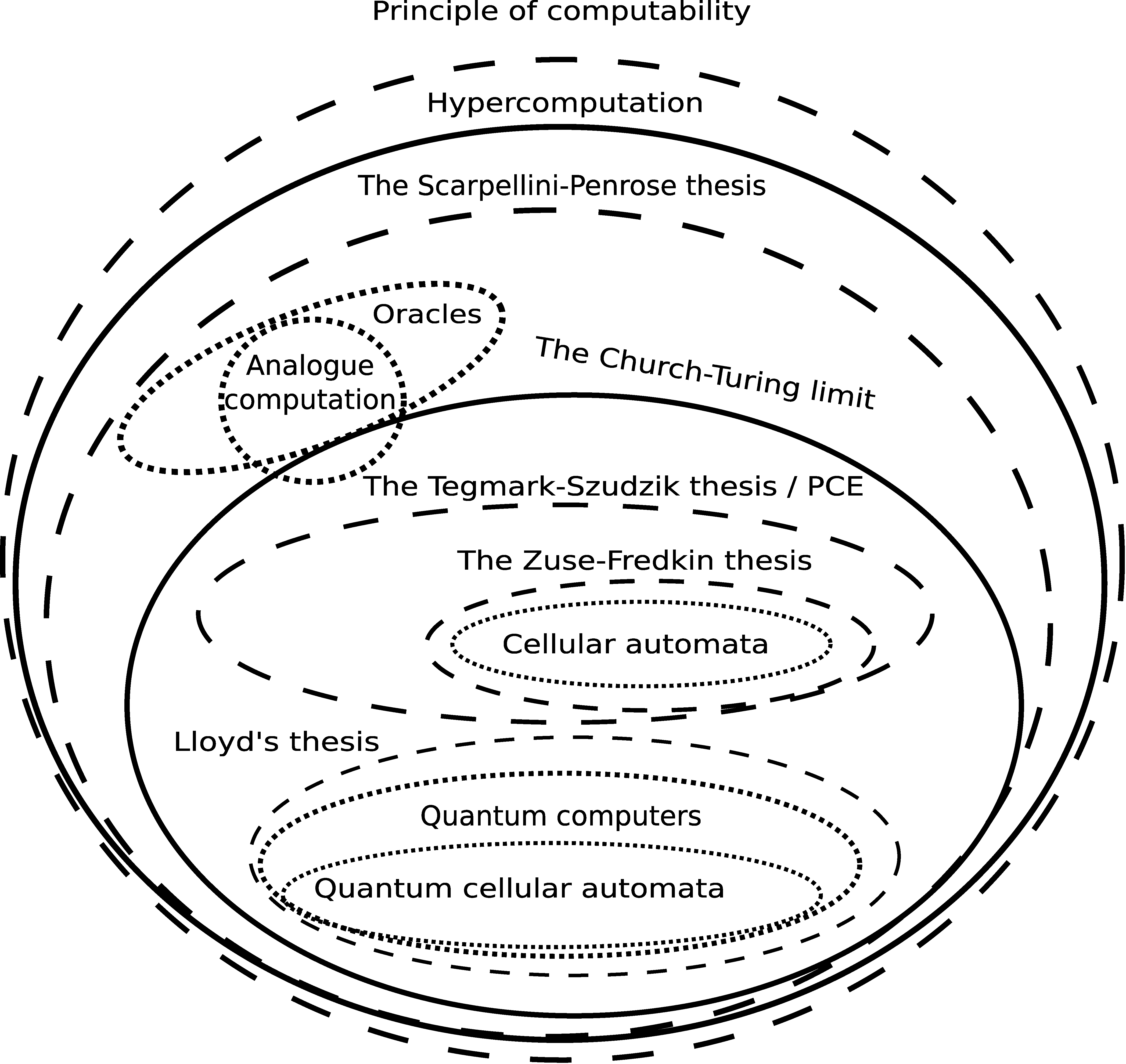
The Church–Turing thesis: a function is effectively calculable if and only if it is computable by a Turing machine or, equivalently, if it is specified by a recursive function.
Given that each computational model can implement 1 a set of functions, we refer to that set as the computational power of that computational model. According to this definition, a computational model has greater computational power than another computational model if the subset of functions that it can implement strictly contains the set of the other computational model, and the two models have the same computational power if both sets are equal. It is interesting to note that the Church–Turing thesis can be divided into two claims: (1) a computational power exists that cannot be exceeded under the finitary point of view, and (2) the limit of what is effectively calculable under the finitary point of view is the computational power of a Turing machine, the Church–Turing limit. The Church–Turing thesis has been supported by additional research on other computational models that found the same limit, e.g., the post-canonical system, semi-Thue system [22], multitape Turing machine [23], random access machine [24], or P-system [25]. A computational model that has the same computational power as a Turing machine is called Turing complete.
Turing’s result that there are functions that cannot be calculated could be discouraging. However, if the Church–Turing thesis is correct, then Turing showed that a unique mechanism could calculate every effectively computable function, and there are infinite functions that could be effectively calculated. This fact is the key to the technological revolution in which we are living because we only need a Turing-complete device to implement any effectively computable function. However, this revolution is not only occurring in the technological world; concepts of computation are permeating physics as well. The use of computational concepts in theoretical physics has been a progressive process. The first person who considered computation statements to have a physical meaning was the theoretical biologist Robert Rosen. He restated Church’s thesis as a physical claim about the nonexistence of a certain class of a physical process [26]. Until Rosen’s paper, the explanations for a physical phenomenon were based on postulate physical entities with specific features in nature. However, Rosen proposed that limitations in computation explain facts about nature. Unfortunately, his ideas came to the scientific community too early because the issue was not under discussion, so his work had little impact at the time.
In the emergence of computer science as a framework for fundamental physics, one element that has greatly stimulated that line of research is the cellular automata model. The idea of cellular automata (CA) came about when Stanislaw Ulam suggested to John von Neumann in the 1940s that he use lattice networks to study self-replicating systems. In addition, Norbert Wiener and Arturo Rosenblueth created CA models to mathematically describe impulse conduction in cardiac systems [27]. These developers of the CA computational model did not have fundamental physics in mind. However, the idea of that relation emerged in the mind of Konrad Zuse, a computer pioneer. First, Zuse proposed in 1967 that the entire universe could be computed by CA [28]. Two years later, in his book Calculating Space [29], he proposed that the laws of physics were discrete, and the entire universe was a cellular automaton. Zuse’s idea was too early, as was Rosen’s, to impact the scientific community in that moment.
Zuse’s idea would not be considered until physicists began to research CA as a tool to study physical phenomena. This began with Tommaso Toffoli, who researched CA under the hypothesis that they provided natural models for many investigations in physics [30,31]. Once CA were used as a mathematical tool, the scientific community began to take an interest in their role in fundamental physics. This interest became evident during the 1981 MIT conference “Physics of Computation” organised by Ed Fredkin, Rolf Landauer, and Tom Toffoli, who believed that physics and computation were interdependent at a fundamental level [32]. Among those at the conference were Richard Feynman and John Archibald Wheeler, and the assistance of these two outstanding physicists was not a coincidence. Many years before the conference, Feynman had stated the following:
“So I have often made the hypothesis that ultimately physics will not require a mathematical statement, that in the end the machinery will be revealed, and the laws will turn out simple, like the chequer board with all its apparent complexities” [33] (pp. 57, 58).
Additionally, Feynman considered that the universe could not be processing an infinite amount of information at each tiny spacetime region [33] (p.~57). His ideas lead him to have a remarkable interest in the nature of computing in the latter part of his career [34], and his participation in the MIT conference is proof of this.
Wheeler, who was Feynman’s mentor, defended the necessity of looking for something more fundamental than spacetime; he called it pregeometry [35]. He defended that necessity because he believed that conventional continuum theories have limited applicability. Additionally, Wheeler’s work emphasised the idea that information was a fundamental element of physics [36].
Beyond the importance of Feynman and Wheeler’s support for using computational concepts in physics, Feynman’s presentation was relevant because it launched the idea of developing quantum computing [37]. Research on quantum computing has been, without a doubt, key to strengthening the idea that computation plays a fundamental role in physics.
In addition to Zuse, who presented related ideas at the 1981 MIT conference, Marvin Minsky presented a paper about the universe as a CA [38]. However, the strongest proponent of Zuse’s idea that the universe is a CA was Edward Fredkin, as Minsky recognised in the acknowledgment section of his paper.
“This essay exploits many unpublished ideas I got from Edward Fredkin” [38] (p. 551).
Although Fredkin wrote about his ideas only several years after the MIT conference [39], he personally encouraged many physicists to research CA in fundamental physics before he wrote his papers, as they have recognised. This influence is why today we speak about the Zuse–Fredkin thesis [40], which states the following:
The Zuse–Fredkin thesis: the universe is a cellular automaton.
Another noteworthy contribution from the MIT conference was the billiard-ball model presented by Fredkin and Toffoli [41]. This model can be used to simulate Boolean circuits, and so it can perform any computational task. They noted in their work that any configuration of physical bodies evolving according to specified interaction laws can be interpreted as performing some sort of computation. However, they also noted that any physical system computes its future state. Here, it is important to note two different views about computation. One is the classical view of computation in nature, in which physical processes allow computing processes [42]. The other view of computation is that proposed by Rosen and Zuse, in which physical phenomena are computational processes and the universe is a computational system. This modern view was also exposed and defended by Toffoli at the 1981 MIT conference [43]. This conference made the scientific community pay attention to the claim that the universe is a computational system.
After the conference, CA became an influential framework to describe physical processes [44,45], and some physicists began to ask whether CA had the answers to fundamental physics questions [46]. One of the most relevant lines of research has been the reformulation of field theory with CA, and work by Tsung-Dao Lee has influenced this research area. He suggested that we should use difference equations as the fundamental equations in physics [47,48,49]. However, not all CA reformulate field theory. Karl Svozil directly addressed the issue of whether quantum fields are CA [50]. He established a connection between CA and lattice field theory, and he showed that the fermion doubling problem appears because of a no-go theorem [51,52,53]. However, as Andrew Ilachinski [54] had previously noted, Svozil did not consider a generalisation of CA with quantum features, and Svozil’s view was more limited than either Fredkin’s [55] or Lee’s [47]. In 1988, Gerard ’t Hooft proposed that field theories at the Plank scale could be formulated through deterministic, local, reversible CA [56], and he has continued developing this line of research [57]. He has developed the cellular automaton interpretation (CAI) [58,59,60], but a full discussion of the CAI is beyond the scope of this paper. Briefly, his work with CA proposes alternative answers to questions without answers by the Copenhagen interpretation providing a new view on the quantum vacuum. As he himself recognises, his theory does not yet answer all questions, but it is controlled by a Schödinger equation which is valid, and therefore his theory is genuinely quantum mechanical [60]. His work shows that determinism is not dead [59,61], and the battle between determinism and indeterminism continues.
In parallel with Hooft’s work, Stephen Wolfram’s work using CA generated an impact in the scientific community. He has defended the computational view of nature, and he has explicitly claimed that “all processes, whether they are produced by human effort or occur spontaneously in nature, can be viewed as computations” [62] (p. 715). In 2002, Wolfram presented the results of 20 years of research in his controversial and widely known book A New Kind of Science [62]. In this book, Wolfram proposed that the nature of computation must be researched experimentally and that understanding it is necessary for understanding the physical world. He stated that programs can be used to describe the natural world and that we need to study the execution of those programs to understand nature. Additionally, he launched a hypothesis about the computational limits of our universe, the principle of computational evidence.
The principle of computational equivalence (PCE): “No [natural] system can ever carry out explicit computations that are more sophisticated than those carried out by cellular automata and Turing machines” [62] (p. 720).
A discovery made while researching CA was that self-organized criticality provides the emergence of scale-free structures [63,64]. The results of CA experiments showed how large-scale structures can emerge in a simple computational model such as the CA. In different CA models, the feature of a scale-free structure was observed, and it matches the observed structure of the universe [65], which has structures in all the scales. These results support the possibility that the Zuse–Fredkin thesis is true.
An alternative line of research to formulate the universe as a computational system is quantum cellular automata (QCA). Gerhard Grossing and Anton Zeilinger started this line of research when ’t Hooft began using CA. They presented a paper in which they defined a quantum cellular automaton to study quantum computing [66]. Although the idea of QCA was proposed by Feynman at the 1981 MIT conference, Grossing and Zeilinger were the first to work on the topic [67,68,69]. They found that “except for the trivial case, strictly local, unitary evolution of the whole QCA array is impossible” [69] (p. 3470). Thus, their models were only partially quantum mechanical. David Meyer proposed the name quantum cellular automata only for CA with exactly unitary, nontrivial, local evolution [70,71]. Meyer and other authors have used QCA to study quantum lattice gases by simulating them [70,72,73]. In 1995, John Watrous defined other QCA to solve the problem of giving a global time-evolution unitary operator [74]. He named them well-formed QCA for which time-evolution operator T is unitary. He did not address the question of determining whether a given quantum cellular automaton is well-formed or not, but he defined the class of partitioned QCA for which checking well-formedness is easy. Shortly after this, a polynomial-time algorithm was discovered that checks whether a quantum cellular automaton is well-formed or not [75,76]. Michael McGuigan generalised the definition of QCA to include bosonic, fermionic, supersymmetric, and spin quantum systems [77]. Research on the Watrous model showed that some instances allow superluminal signalling [78]. Alternatively, other QCA models have been proposed which avoid superluminal signalling [78,79,80]. Another topic that has been addressed is the reconstruction of the geometry of Minkowski spacetime and the free dynamics of relativistic quantum fields [81]. This problem has been addressed through the notion of fermionic QCA [82], and Mauro D’Ariano et al. have obtained multiple results on this topic [83,84,85,86,87]. More details about these QCA results can be consulted in a recent review [88].
Here, it is important to note that although QCA could be considered an extension of CA because they add features with regard to the former, they are two completely opposed views about the nature of the universe. The Zuse–Fredkin thesis is the core of CA research, whereas the idea that the universe is a quantum cellular automaton is fundamental to QCA research. These two proposals are completely different. CA research proposes to explain the weird features of the quantum world through CA which are discrete and deterministic. However, QCA research assumes that the weird features of the quantum world do not emerge from but are instead fundamental properties of our universe. Although some scientists underestimate the Zuse–Fredkin thesis because it assumes determinism, the work done by ’t Hooft has shown it is a line of research [58,59].
It should be noted that a cellular automaton is one specific computational model. It is possible the universe could be ruled by another computational mechanism. However, whether the most elemental level is a cellular automaton or another computational model which has the computational power of a Turing machine, there are some limitations that would exist in nature. These general limitations are inferred from Gödel’s works and the connection between logic and computation [89].
On the other hand, our technology—and we do not know whether nature as well—allows us to calculate functions only within the Church–Turing limit. This creates an issue regarding whether our physical theories are within or beyond the Church–Turing limit. This was initially posed and investigated in the early 1970s by George Kreisel [90], who wanted to distinguish theories according to whether they are computable by a Turing Machine or not.
In 1985, Wolfram, considering Turing’s theorem that there is no Turing machine that can determine whether any other Turing machine halts or not, proposed that a physical system can have a property he called computational irreducibility. If a physical system is computationally irreducible, then there is no shorter process that can predict its physical behaviour than its physical behaviour [62,91]. Computational irreducibility is an important link between computation and physics because it establishes an interpretation of what it means physically when a function is uncomputable. The concept of computational irreducibility explains that when a problem regarding calculating the value of a physical system’s property is uncomputable, the complexity of the system’s evolution is so high that developing any effective method to calculate with absolute precision the system’s evolution is impossible. A physical system being computationally irreducible would be directly connected with the fact that the system is capable of universal computation and the computational limit for physical systems stated by the PCE. This would happen because predicting the behaviour of a system requires creating another system, a predictor, that carries out a computational process that calculates the future state from the initial state, and the PCE limits the computational power that a predictor can have. Thus, according to Wolfram, the PCE would be what causes us not to be able to create a predictor to calculate the behaviour for some physical systems. The existence of computational irreducibility has been found in dynamical systems [92]; Toby Cubitt et al. have achieved an outstanding result in the spectral gap problem by achieving a proof of being an undecidable problem [93], and Eva Miranda et al. have recently shown that there is no algorithm to determine whether a fluid particle will pass through a specific space region in finite time [94]. Wolfram has also speculated that “computationally reducibility may well be the exception rather than the rule” in physics [91] (p. 735), and this fact would justify the necessity to study many physical systems by executing programs that replicate the evolution of those physical systems [62].
At the same time that Wolfram gave a physical interpretation for a function that is uncomputable, David Deutsch, unaware of Rosen’s proposal, proposed that the Church–Turing thesis should be considered a physical principle [95]. Deutsch went further than Kreisel because he was not speaking about a feature of the theories but about it as a feature of nature itself. Thus, Deutsch formulated the following physical principle:2
Deutsch’s principle:“Every finitely realizable physical system can be perfectly simulated by a universal model computing machine operating by finite means” [95] (p. 99).
It must be noted that Deutsch’s principle is not by itself determining that every physical system can be simulated by a Turing machine. Although Deustch’s proposal is like Rosen’s, the background of Deutsch’s proposal is different. Rosen looked for justification in classical physics, but Deustch’s arguments emerged from quantum physics, and he defined a quantum Turing machine3 to elaborate his arguments. The formal definition of a quantum Turing machine had a dual value: it supported a statement about fundamental physics, and it opened the door to quantum technology.
The interest in quantum technology has been an important motivation to address the physical limits of computation. In 1998, Norman Margolus and Lev B. Levitin presented the Margolus–Levitin theorem [97], a fundamental limit on the maximum speed on quantum computation. Later, using the Margolus–Levitin theorem, Lloyd calculated the capacity of computation of a physical system with a mass of one kilogram confined to a volume of one litre [3] and the capacity of computation of the universe [98].
In the 1990s, two new connections between computation and physics emerged in the field of relativity. One of those connections started in 1990 when Itamar Pitowsky developed the idea to use relativistic effects to solve unsolvable problems with a Turing machine [99]. He defined what is now known as Pitowsky spacetime. In 1992, Mark Hogarth generalised Malament’s ideas about requisite spacetime structures and defined what we know as Malament–Hogarth spacetime, and he applied this to computability theory [100,101]. The other connection emerged in the field of relativity also started in 1990 when John Friedman, Michael Morris, and other colleagues questioned what would happen if a computer could access closed time-like curves (CTCs), and they began to study that possibility [102]. In 1991, Deutsch showed that CTCs do not inevitably imply logical inconsistencies such as the grandfather paradox, but he pointed out that if CTCs existed, they would have direct consequences for computational processes [103]. Deutsch’s proposal opened the door to a new model of computation in which a quantum computer has access to a CTC. In 2003, Todd Brun showed that CTCs can be utilised to solve problems efficiently, which is considered impossible in the classical model [104]. In 2004, David Bacon demonstrated that the new computational model could efficiently solve computational problems generally thought to be intractable [105]. A year later, Scott Aaronson defined computational classes assuming CTCs and studied some possible relations between the new complexity classes and others already well-known. In 2008, he succeeded in determining the computational power for quantum computers with CTCs [106]. Recently, Aaronson and his colleagues addressed what Turing machines compute in closed time-like curves [107], and even the effects of different kinds of CTCs on computational processes have been analysed [108]. The link between general relativity and computation has led to the development of the theoretical field of relativistic computers [109,110,111,112]. Although this is a theoretical field, a new kind of prediction of general relativity emerges from it, and perhaps if the discovery of the Alcubierre warp drive metric in the real world [113] were confirmed, those kinds of predictions might one day be put to the test.
One final field of physics to mention regarding where the concept of computation has penetrated is hydrodynamics. Christopher Moore posed the question of whether hydrodynamics is capable of computation in 1991 [114], but only recently, as mentioned above, have Miranda et al. shown the existence of undecidable particle paths of three-dimensional fluid flows [94]. In addition, it is remarkable that Terence Tao has begun a program to understand the solutions to the Navier–Stokes equations by using computational concepts [115,116].
Usually the word computation references any calculation that does not break the Turing machine limit, but there is no logical reason to say that something beyond this limit cannot be physically calculated. Turing himself researched the idea of devices that can break the Turing machine limit [117], and that work created a theoretical field many others have since explored. Different researchers have addressed the possibility that processes beyond the Turing limit happen in nature (see [118] for a historical overview of this research). In 1963, Bruno Scarpellini speculated that processes beyond the Turing limit might occur in nature [119], but Roger Penrose has been the greatest promoter of the idea that physical processes exist in nature that imply a computational power beyond the Turing limit [120,121]. Considering Scarpellini’s and Penrose’s ideas about computational processes that happen in the universe, we deem it appropriate that the following thesis bear their names:
The Scarpellini–Penrose thesis: In the universe, physical phenomena exist that involve a computational power beyond the Turing limit.
Although no proof exists that the Scarpellini–Penrose thesis is true, multiple theoretical works consider processes beyond the Turing machine limit. For example, in 1995, Hava T. Siegelmann presented a computational model with computational power beyond the Turing machine limit [122]. The model, called the analogue shift map, connects computer science and physics because it can be considered a natural model of chaotic (idealised) physical dynamics.
In 1999, Brian Jack Copeland and Diane Proudfoot introduced the term hypercomputation [123], which is now commonly used in the field, to describe calculations beyond the Turing machine limit. However, hypercomputation is only a theoretical concept, and its existence in nature is a matter of debate. For example, Martin Davis has strongly denied its existence [124,125]. The debate about hypercomputation is one of the best examples of how computation has moved from the mathematical field to the physical field, and what is true without a doubt is that the discussion about hypercomputation’s existence drives further testing of quantum and relativistic concepts.

2.1. Computational Complexity

So far, we have discussed how the concept of computational power broke into the field of physics. However, in computer science, another issue emerged—that of computational complexity—after the release of the results regarding algorithmic computational power and its limit.
Since the Middle Ages, work has been done on optimising arithmetic algorithms and reducing the number of operations required to calculate the value of some functions [126], but the appearance of digital computers increased the interest in and importance of understanding the difficulty of calculating a computable function. In 1960, Michael Rabin addressed what it means to say that one function is more difficult to compute than another [127]. Shortly after, Juris Hartmanis and Richard Stearns coined the term computational complexity [128]. The idea behind this concept is that the problems can be divided into different classes for which the amount of resources required to resolve them does not depend on how cleverly the algorithm is designed to carry out the calculations but on the problem itself. Each of these classes is called a complexity class. These cited works, along with others, made analysing algorithmic complexity emerge as a scientific subject in the 1960s.
Among the different options for measuring computational complexity, the complexity classes usually measure temporal complexity or spatial complexity. Also, the classes are initially defined using one specific computational model. On the basis of the definitions of the complexity classes, the field of computational complexity emerges, and one of its main challenges is proving the equality between the complexity classes defined using different computational models and other set-theoretic relations between them. Studying the computational complexity in different computational models gave rise to several hypotheses, such as the sequential computation thesis, the parallel computational hypothesis [129], the extended parallel computational hypothesis [130], and the strong Church’s thesis [131]. The discussions about these hypotheses showed the importance of the restrictions on the operations and features of computational models in accepting or rejecting these theses [132]. Additionally, researchers have proposed and investigated the existence of computational complexity hierarchies (or complexity classes hierarchies) [133]. A computational complexity hierarchy is a classification of the complexities classes according to the set theoretic relations (e.g. strictly contained and equal) that exist among them. One of those hierarchies is the polynomial hierarchy (or polynomial-time hierarchy) that generalizes the classes P, NP, and coNP. Computational complexity is a field in which large gaps still exist regarding the relationships between the complexity classes. For example, we do not have proof that the polynomial hierarchy does not collapse; it is only a conjecture.
Feynman’s claim that building a quantum computer would be a qualitative leap in the technological capacity of computation (because a Turing machine cannot efficiently simulate a quantum system) has triggered another link between physics and computation because it has led to exploring the computational complexity of quantum computational models [134,135]. Deutsch’s paper, mentioned above, showed that the computational complexity hierarchy is different when considering the quantum Turing machine’s computational model. Bernstein and Vazirani began to study the computational complexity of the quantum Turing machine [136] and the class BQP (bounded-error quantum polynomial time) [137]. Additionally, a connection between computation and physics emerged when they stated that computational complexity theory rests upon the thesis that a reasonable model of computation can be efficiently simulated on a probabilistic Turing machine [136]. This thesis has been named the extended Church–Turing thesis [138] (also known as the strong Church–Turing thesis [133]).
The extended Church–Turing thesis: Every physically reasonable computational device can be simulated by a Turing machine with at most polynomial slowdown.
It must be noted that when Bernstein and Vazirani were formulating the extended Church–Turing thesis (CTT-E), they were formulating a veiled thesis that claims that the CTT-E is wrong and that it emerges from Feynman’s paper [37]. We could formulate Feynman’s proposal as a thesis:
Feynman’s thesis: There exists a quantum computational device that cannot be simulated by a Turing machine with at most a polynomial slowdown.
Showing that Feynman’s thesis is correct (and that the CTT-E is wrong) is an important topic known as quantum supremacy [139,140]. In addition to the large technological leap that would happen if Feynman’s thesis were true and the quantum computer that could be built with the imagined computational capacity, Feynman’s thesis is relevant to physics because it implies that quantum systems can only be simulated using quantum computers. Although, in 1996, Seth Lloyd showed that each quantum system could be simulated by a quantum computer [141], simulating quantum systems using quantum computers involves studying the complexity of quantum algorithms to know whether their computational complexities are barriers that prevent the quantum systems being simulated by the current quantum computers [142,143,144]. Therefore, computational complexity emerges as a key element for understanding quantum systems. In addition, we cannot fail to mention the new results presented by Zhengfeng Ji et al. that establish the limits of verifying answers to computational problems using multiprover interactive proofs [145,146]. These results have been obtained by relating quantum entanglement and computing, and they resolve Tsirelson’s problem in the negative. If their proof is correct, it shows another link between fundamental physics and computation.
Proof of the relevance of quantum supremacy to current research topics is that governments and large companies are carrying out extensive projects to build a quantum computer, and these projects are mainly based on assuming that Feynman’s thesis is correct. Different theoretical investigations on computational complexity have been done by considering different quantum computational models [147,148,149], and projects also exist that provide experimental evidence that quantum computers cannot be efficiently simulated by classical computers [134,135,150]. Quantum supremacy has emerged as a bridge between theoretical computer science and physics [151,152], but this connection also requires an enormous amount of work in developing quantum computing technology [153]. Difficult technological issues exist, such as quantum measurement [154], the scalability of quantum processing [155], and algorithmic improvements that reduce the required hardware [156].
The current state of the art in quantum computational technology has been denominated Noisy Intermediate-Scale Quantum (NISQ) [157]. A NISQ device contains a number of qubits ranging from 50 to a few hundred and lacks quantum error correction. The NISQ is being used for optimization problems, machine learning, and neural networks [158].
Regarding the challenge of achieving quantum supremacy, John M. Martinis and his team announced in 2019 that they achieved quantum supremacy by doing a task which, according to them, would require 10,000 years on a classical computer [159]. However, at IBM, Edwin Pednault et al. argued that an ideal simulation of the task from the Martinis team’s experiment can be performed on a classical system in 2.5 days and with far greater fidelity [160]. The race to achieve quantum supremacy continues; Jian-Wei Pan and his teams have surpassed the Google team in computational capacity [161,162,163], and new advances toward quantum supremacy and a quantum computer have been made [164,165]
However, despite great achievements in quantum technology, no proof of Feynman’s thesis exists because no one has mathematically proven that no fast-classical algorithm exists that could deny the claim of quantum supremacy in those experiments. In this technological time, we have only succeeded in applying quantum annealing to resolve sampling and optimization problems, and quantum annealers have their physical limits [166,167]. In addition, we do not know whether quantum mechanics is the final theory needed to understand the microscopic world, but if it is the correct one, no-go theorems emerge from it that affect quantum computing [168]. A method has also been recently achieved to execute a quantum computing algorithm on a classical computer [169]. These issues show that we do not know much about the relations between the limits of classical and quantum computational models, and the race to build a quantum universal computer also continues.
Different researchers have noted that computational complexity offers a new regime in which to test quantum mechanics [42,170]. Until today, all aspects of quantum mechanics that have been experimentally studied can all be classified as low complexity quantum mechanics because we can calculate the results of the experiment using technology that uses classical computational models. However, it is not clear how quantum mechanics should be tested in the high complexity limit. We cannot calculate the correct result using the technology based on classical computational models because it would require more time than we will be alive. Because of this problem, there is discussion about whether it is theoretically possible or whether there are fundamental obstacles that prevent such testing. One framework that has been proposed to address the testing of quantum computers is using the concept of computation through interaction [138,171].
Another important connection between physics and computation has emerged by studying computational complexity using a quantum version of the Boolean circuit model, which Deutsch proposed as an alternative quantum computational model to the quantum Turing machine [172]. Andrew Chi-Chih Yao proposed using the quantum circuit model to develop a complexity model similar to that of a Boolean circuit model [173]. The quantum circuit model allows obtaining new results about the relation between classical computational complexity and quantum computational complexity. This kind of measure of computational complexity has been named gate complexity. Later, Michael A. Nielsen and colleagues created a method to calculate the gate complexity of a quantum algorithm through finding the shortest path between two points in a Riemannian geometry [174,175]. This alternative method to calculate computational complexity has been named geometry complexity. One important result that was found while studying computational complexities in quantum computational models is that the classical polynomial hierarchy collapses to its third level if quantum computation exists [176].
The developments of building and studying a quantum computer have allowed the introduction of computational complexity into different issues of physics, one of which is the landscape of the multiverse obtained by string theory [177,178]. However, the field most impacted by these theoretical results about computational complexity is fundamental physics, in which a revolution is happening. This progress started within the theoretical study of black holes when Daniel Harlow and Patrick Hayden launched the idea that the solution to the firewalls in the event horizon could be related to their computational complexity. They addressed quantifying the difficulty of decoding Hawking radiation by using quantum computational complexity [179]. Leonard Susskind has taken the importance of computational complexity seriously, and he is researching the topic and motivating his colleagues to employ and research the concept as well [180]. Susskind has claimed that to understand the properties of black hole horizons, it is essential to consider quantum computational complexity [181]. He has advocated the existence of a connection between Nielsen’s approach and holographic complexity, and he and his collaborators have developed two new gravitational observables with regard to quantum computational complexity: complexity = volume conjecture [181,182] and complexity = action conjecture [183,184]. In addition, the computational complexity language has been used to address the time-energy uncertainty relation [185] and propose the existence of a thermodynamics of quantum complexity [186]. This has given rise to important research activity on field theories employing quantum computational complexity [187,188,189,190,191,192,193].

2.2. A Computational Characterization of the Universe

Before continuing with how computation entered the field of physics, we must remember that the computational power of two computational systems can be compared using the set of functions that each one can implement. They have the same computational power if they can implement the same set of functions. One system has less computational power than another if its set of functions is a strict subset of the set of functions of the other system.
Regarding the computational power and the computational complexity hierarchy that a physical system can have, the physical systems are divided into three main classes from a computational view in the literature: computable, supercomputable, and hypercomputable. These values can be split into additional classes with specific mathematical definitions, but the academic literature refers mainly to these three values of computational power in broad discussions on the subject. Because we intend to carry out a broad discussion about the phenomenon of computation, we will employ these three values to establish the three following classes:
  • Computational systems. Systems that cannot go beyond the Turing machine limit.
  • Supercomputational systems. Systems that have the classical computational limit of the Turing machine but can solve nondeterministic polynomial time problems in polynomial time.
  • Hypercomputational systems. Systems that have a computational power beyond the Turing machine limit and can therefore solve at least one problem that is noncomputable by the Turing machine model (e.g., the halting problem).
The idea of a machine capable of carrying out a function beyond the Church–Turing limit is not against the works of Turing because it was an idea from Turing himself; he called it an o-machine, and it is characterised by the fact that it contains an oracle [117]. An oracle would be an object that produces the correct output in a single step to a function that cannot be calculated by a Turing machine.
It should be noted that there is abuse of the word computational in the literature. It is sometimes used to describe systems that calculate functions that can always be calculated by a Turing machine. Other times, it is used to identify any system that carries out calculations, regardless of whether the system fulfils the finitary point of view or whether it carries out calculations beyond the Turing machine limit. For example, Copeland et al. discuss whether the universe is a giant computer, but they are only against this claim when it has a narrow meaning of computational system because they defend the possibility of a hypercomputational process in the universe [194].
As we have already mentioned, Zuse was the first to propose that the universe is a computational system, and he pointed out a specific computational model. Another less specific possibility is making a computational characterisation of the universe without determining which computational model the universe is. In the previous subsection, we mentioned three classes of physical systems defined by their computational features. The universe is a physical system, so the universe must belong to one of those classes. Depending on the computational features of the machinery that rules the universe, our universe should be one of the following:
  • A computational universe.
  • A supercomputational universe.
  • A hypercomputational universe.
Lloyd has formulated a proposal that agrees with Zuse’s proposal in considering the universe to be a computational system but differs regarding the kind of computer.
Lloyd’s thesis:4The universe is a quantum computer [98,196,197].
Another hypothesis about the computational nature of the universe was formulated in 2008 by Max Tegmark [198]. He formulated the computable universe hypothesis, and he connected it with the external reality hypothesis and the mathematical universe hypothesis. These hypotheses claim the following:
The External Reality Hypothesis (ERH): there exists an external physical reality completely independent of us humans.
The Mathematical Universe Hypothesis (MUH): our physical reality is a mathematical structure.
Computable Universe Hypothesis (CUH): the mathematical structure that is our external physical reality is defined by computable functions.
The CUH contains the ERH and the MUH, but it also goes further because it fixes a boundary that determines a set of mathematical structures among which would be our universe. It must be noted that the CUH uses the same computational limit to establish the boundary as the computational limit proposed by the PCE for the nature. Additionally, if the Zuse–Fredkin thesis is true, then the CUH and the PCE are true. However, if the CUH is true, it does not imply that the Zuse–Fredkin thesis is true because a cellular automaton is only one of the many computational models that have the computational power of a Turing machine.
Independently of Tegmark, Matthew P. Szudzik also proposed the CUH in the following way [199,200]:
Computable Universe Hypothesis: the universe has a recursive set of states U. For each observable quantity, there is a total recursive function ϕ. ϕ ( s ) is the value of that observable quantity when the universe is in state s.
Tegmark’s use of the term computable is synonymous with recursive. Thus, the proposals of Tegmark and Szudzik are the same. Although both authors named their proposals the computable universe hypothesis, we are going to reference it as the Tegmark–Szudzik thesis. We will explain this decision in Section 7. It must be noted that while Lloyd’s thesis proposes a supercomputational universe, the Tegmark–Szudzik thesis proposes a computational universe. We are not aware that Copeland or any advocate of the existence of hypercomputation in nature has explicitly proposed that our universe is a hypercomputer, but they could make this claim if the existence of hypercomputation is assumed.
This year, the London Institute for Mathematical Sciences celebrated a one-day symposium for physicists and mathematicians to select the most important mathematical challenges for the 21st century, and one of the challenges they selected is asking “Can Tegmark’s mathematical universe be made rigorous?”5

3. The Link between Physics and Computer Science

We have seen that the concepts of computation have profoundly entered the field of physics, but in the face of that fact we must ask ourselves why that is the case. Is it just a matter of fashion or is there any deep reason for this? The answer is that there is a deep reason that is rooted in the fact that the concept of state underlies both the conceptualisation of computational processes and physics’ conceptualisation of the universe. Below, we clarify this point, which is fundamental to the rest of the paper. Firstly, we need to pay attention to the concepts of function and computable function.6 Given a set D, named domain, and a set C, named codomain, a function f is a subset of the Cartesian product D × C that fulfils that if ( x , y ) D × C , there is not any ( x , z ) D × C where y z . On the basis of the previous definitions, we can define a set F as the set of all functions corresponding to the sets D and C.7 Secondly, we must note that a machine M L whose operations fulfil a list of limitations L can compute a function f if for all x that belong to D, M L ( x ) = f ( x ) , so the output value the machine computes from x is the same value as the image of x by f.8 Therefore, we can define the set of all computable functions by M from D to C, and we name it computational space9 and denote it by M D C L . The M D C L is the computational power of the machine M L from D to C. In addition, we say that M D C L is a limit computational space if no other machine M exists that fulfils L and whose computational space M L D C has a function f which is not in M D C L .
The work of Turing shows that when D and C are the positive integers, L is the finitary point of view, and M is the Turing machine; then, the computable space of the Turing machine is smaller than the set of the functions on the domain of positive integers. Thus, there are functions on the positive integers that are not computable by a Turing machine.
It must be noted that there is not only one limit computational space because each combination of a domain, codomain, and list of limitations for the operations generates a set of functions. We use ( D , C , L ) -computational space to name the set of computational functions that correspond to the union of all the sets of computational functions from C to D of all the machines that fulfil the list of limitations L . Thus, when Turing found a limit in the computational power, ω -computability, he obtained the limit computational space that belongs to the finitary point of view. If the list of limitations on the operations that must fulfil a computational model is modified, other computational models can be devised that have different computational power [201] and show and determine other computational spaces [202]. For example, if the list of limitations allows infinite objects, the α -Turing machine is accepted as a computational model, and the computational power of this computational model is α -computability [203].
Having presented the previous concepts, we are ready to discuss the strong link between physics and computation. This connection resides in the fact that physical theories are built on the concept of state [204], and the set of physical states can be considered as a domain and a codomain. The set of physical states has an associated specific set of functions, which can be interpreted as the possible physical laws that could rule the physical system because it contains all the ways in which the physical system could evolve. Thus, the evolution of the universe is described by one function of the space of functions of the set of its states. Additionally, given that the physical evolution of the state of the universe happens, the function that describes that process is a computable function with regard to the computational power of the universe. Therefore, physics and computer science are completely connected because the concept of state superimposes these two fields. One especially noticeable example that shows that the concept of state connects physics and computer science is the Margolus–Levitin theorem.
A reader might think that the link between physics and computation is not very strong because although mathematics allows us to use sets to describe the states of a physical system, not every set describes a space of states of a physical system. Although it is correct that every set does not describe a space of states of a physical system of our universe, that fact does not weaken the link between physics and computation because the fact that the number of sets being greater than the number of physical systems that our universe contains is indeed key to our understanding of nature. For example, physics can address how our universe would be if any of its fundamental features were different because for that kind of research, the diversity of sets allows finding one to represent the space of states necessary for studying a hypothetical universe.

4. Arguments against a Computational Universe

Until now, the proposal that the universe is a computational system has been considered provocative in the field of physics. However, we argue that this is far from true because, in fact, computability underlies physics’ conceptualisation of the universe.
In the second section, we saw that one of the most important claims of the new computational view is that the universe is a computational system. This claim has generated controversy, and, in this section, we discuss seven arguments against it. The easiest strategy to prove that the claim is false is to show that a non-computational physical process exists. Even if only one non-computational physical process existed, the claim would be false, and given that the universe is a physical system composed of physical systems, the claim would be false.
For this discussion, we show that there is a misconception in that strategy because the term non-computational does not express a feature in absolute terms, and to have a complete meaning, it always requires a context. Specifically, it is used to refer to a function that is in a space of functions and is not in a computational space defined by a computational model on that space of functions. This implies that it is necessary to fix a computational space, that is, the context, so that one can claim that a function is non-computational. Thus, it is wrong to use the term non-computational in absolute terms because it expresses a condition with reference to a specific (limit) computational space. For example, if a process can be described with a function beyond the limit of a Turing machine and we use the term non-computational, we are implicitly given the context of the computational space defined by the Turing machine model. If the context accepts hypercomputational processes, the same function cannot be qualified as a non-computational function in that context. We will discuss the concept of non-computational in further detail below.

4.1. The Argument of Radioactive Systems

The first argument against the claim that the universe is a computational system was proposed even before Zuse announced the idea in 1967. The counterargument can be found in the paper written by Rosen in 1962 [26]. He mentioned an example that George Yuri Rainich gave him in which a physical system is computationally indescribable. The physical system contains radioactive material, and the output produced by the system depends on the particle emission, so it cannot be generated computationally because of the randomness from the radioactive decay. Rosen tried to address this problem by suggesting that the computational view of physical processes only applies to those that have an input, but this manner of addressing the problem involves the universe being non-computational because of the existence of radioactive decay. Szudzik has addressed the radioactive systems example by using the many-worlds interpretation and calculating all possible evolutions of the initial state [200]. One can calculate the probability of each final state by using all generated trajectories, and this probability agrees with the conventional theory of radioactive decay. However, we propose another reason to invalidate the argument of radioactive systems. When Rainich suggested his example to Rosen, probabilistic computation had not yet been considered. The definition of the probabilistic automaton was developed in 1963 by Michael O. Rabin [205], and the definition of a probabilistic Turing machine was developed in 1969 by Eugene S. Santos [206]. The claim that a Turing machine cannot describe a radioactive system is correct because a Turing machine is a deterministic system, and a radioactive system is random. However, deterministic computational models are not the only computational models. We know of many probabilistic computational models—for example, the probabilistic Turing machine—that could accomplish this. Thus, this argument against a computational universe is wrong because it considers computation to be limited to deterministic computation when, in fact, the computational framework is broad and includes probabilistic computation as well. If the universe is a computational system, it can run deterministically or randomly, and computer science has computational models to describe both kinds of state changes.

4.2. The Argument of the Continuum

Another argument against the claim that the universe is a computational system lies in the idea that nature is a continuum. David Tong has attacked the idea that computation plays a fundamental role in nature because he argues that nature is a continuum domain from which discreteness emerges [9]. According to Tong, the laws of physics are not discrete. He claims that the Schrödinger equation does not determine that the universe is discrete but that the discreteness is generated by it, and fundamental particles are ripples of continuous fields. Therefore, the discreteness of particles would not be a fundamental feature of nature but would instead emerge. A consequence of this claim is that it is wrong to state that the similarity between the discreteness of different aspects of nature and digital computers is not casual.
The debate about whether nature is discrete or continuous dates to ancient times, and references to atomism and atoms can be found in both Greek and Indian antiquity. The creation of infinitesimal calculus by Newton and Leibniz and its applicability to physics biased the debate toward continuity [207]. However, with the birth of quantum physics at the beginning of the 20th century, the debate has been biased toward discreteness. Tong has proposed that this debate could be reformulated as computational versus non-computational if computational implies discreteness and non-computational implies continuum. It is beyond the scope of the article to address whether nature is discrete or continuous, but we would like to note that there is a problem with this argument because it is incorrect to reformulate the debate in computational terms. Many scientists believe that the computational power of the mechanism ruling the universe agrees with the finitary point of view and that discreteness is one of its properties [7]. The origin of identifying computation with discreteness comes from the fact that effective calculation in the finitary point of view involves discreteness. However, the finitary point of view is not the only possible set of rules to determine what is an acceptable computational model. If the set of rules allows continuum domains, there are other computational models that emerge.
The first theoretical model of analogue computing was proposed by Claude E. Shannon in 1941 [208], but for a long time after, there was no coherent theoretical basis. Analogue computers did not improve for a while, but this has changed. In 1996, Christopher Moore developed a new approach that has been very successful. He defined a set of recursive functions on the real numbers, similar to the classical recursive functions on the natural numbers, called R-recursive functions [209]. This approach has produced many new results that show that there is a foundation for real recursive function theory [210,211] and a robust notion of ordinary differential equation programming [201,212,213]. Moreover, continuous versions of λ -Calculus have been created [214,215], and recently, a definition of algorithms that allows capturing continuous behaviour has been proposed [216]. In this context, too, it must be noted that Susskind has addressed the issue of measuring discretely or continuously the quantum computational complexity [217].
Currently, people can only find digital computers in the general market, which perhaps creates the incorrect perception that computers are built using only digital technology and causes many people to identify computation with discreteness. Making this assumption is incorrect, however, because commercial analogue computers already existed in the 1960s [218], hybrid systems that employ digital and analogue computation have been developed [219], and creating analogue computers continues to be a current technological topic [220].
Given that computational models with continuous domains exist, computation does not imply discreteness because it is not defined by an absolute criterion; computation is relative to the domains and the set of restrictions that determine which operations are allowed. If an experiment determined that nature is continuous, it would not maintain that the claim that the universe is a computational system is false, but that we should discard the discrete computational models.

4.3. The Counterargument of Evaluation

Giuseppe Longo and Thierry Paul are against the concept that physical processes compute [11]. They have identified computations with equations and believe that in physics, solving equations is only one method to describe physical dynamics. They highlight evaluation as an important method behind the principle of least action and the path-integral, which is different from solving equations. They make the following claims:
“This principle of least action does not ask to solve an equation, it just asks to evaluate the functional S at any possible path γ and select the extremal one” [11] (p. 252).
“But the Feynman ‘path integral’ formulation of quantum mechanics creates a revival of this idea of evaluating instead of computing” [11] (p. 252).
However, this argument is wrong because their classification that distinguishes operations that solve an equation from those that evaluate and select an equation is erroneous. Assuming that evaluating and selecting are non-computational operations is not correct because all the operations are computational, even though they belong to computational models other than the Turing machine. We can see this when using the rewriting system theory as a framework to describe computational models [221,222]. For example, any Turing machine can be translated into a finite term rewriting system, and several declarative programming languages are based on term rewriting [222]. In the rewriting system theory, operations to solve equations and to evaluate and select are all considered rewriting. Operations to resolve an equation produce a reduction process that terminates, and the formal norms are unique. Evaluating and selecting are rewriting rules: evaluating has the features of termination and confluence, and selecting the extremal is an important computational operation, called the minimisation operator, in recursive function theory. The minimisation operator, μ , can be defined on integers and real numbers [209]. Thus, evaluating and selecting are computational operations, and the counterargument of evaluation is wrong.

4.4. The Argument of Infinite Dimensions

Longo and Paul also provided another argument against physical processes being computational. They argued that in quantum mechanics an infinite-dimensional Hilbert space is necessary to represent any continuous observable phenomenon such as position or angular momentum [11]. The reason for using an infinite-dimensional Hilbert space is as follows: in any finite-dimensional space, the canonical commutation relations [ x , p ] = i 1 are not achievable because x and p are trace-class operators in finite dimensions, and the trace of their commutators must vanish. This leads to the conclusion that we have a space for which the identity’s trace is not well defined and must be infinite-dimensional [223]. Longo and Paul believe that this shows that the universe is not describable computationally. Although some alternative proposals have provided finite treatment [224,225], we do not want to engage in discussions about the physical validity of the use of infinite-dimensional Hilbert spaces because we can show that the argument of infinite dimensions is wrong. The error in this argument is that calculating using infinite dimensions is not outside the computational framework. For example, the Turing machine model can be extended to allow an infinite number of tapes or an infinite number of read/write heads [226]. In fact, different infinitary computational models exist that allow computation on ω -strings [203,227]. Thus, calculation in an infinite-dimensional Hilbert space can be included without difficulty in the computational framework.

4.5. The Argument of the Lagrangian Schema

Ken Wharton proposed another argument against the claim that the universe is a computational system in which he states that computation is a process that can only exist in the Newtonian Schema [10]. The Newtonian Schema consists of mapping the physical world onto some mathematical state, using dynamical laws to transform it into a new state, and finally mapping the resulting state back onto the physical world. Most physical theories follow the Newtonian Schema, but Wharton argued that this is not the only way to develop a physical theory and that our universe could not be a Newtonian Schema Universe. He proposed that there is at least one alternative to the Newtonian Schema, called the Lagrangian Schema, which is inspired by Lagrangian mechanics.
The Lagrangian Schema maps the physical world onto a space of states and proposes that nature looks for and follows a specific path between an initial and a final state. The initial and final states are constrained parameters, and the path from the initial state to the final state is an unconstrained parameter. To find the specific path among all the possible ones, a global rule is used. One example of a phenomenon explained using the Lagrangian Schema is light travelling between two points. This phenomenon is explained by Fermat’s principle, which states that the path a ray of light takes between two points is the path that can be travelled in the least time.
On the basis of the above issues, Wharton has elaborated his argument as follows. First, the Newtonian Schema is challenged by the quantum nature of the world. Second, the Lagrangian Schema can better address these challenges presented by the quantum nature of the world. Finally, if the universe is a Lagrangian Schema Universe, then it is not a computational system because it does not calculate like a forward-running (imperative) computer program. This argument is directly connected to the argument in Section 4.3, but while Longo and Paul’s argument is focused on the mathematical nature of the operations, Wharton points out the evolution of the universe as the key issue. This argument could be considered more important now, after the experimental observation of exotic looped trajectories of photons in three-slit interference [228].
Again, we are not going to go into the physical dispute; we do not take sides about whether the Lagrangian or Newtonian Schema can better address the quantum nature of the world, but we disagree with Wharton’s conclusion that denies that the universe is a computational system based on the Lagrangian Schema. In fact, Toffoli argued that the action integral in physics measures the amount of a system’s computation [229], which dismantles Wharton’s argument because he shows that the mathematical apparatus of the Lagrangian Schema can be interpreted as a measure of the computational capacity. However, in addition to Toffoli’s computational interpretation, there is another reason why Wharton is making an incorrect claim when he asserts that only physical theories belonging to the Newtonian Schema are computational—while it is true that the Newtonian Schema can be identified with the imperative paradigm, the imperative paradigm is not the only one. There are computational processes that belong to other computational paradigms, among one of which is logic programming that involves unknown values as variables [230]. A program written in a logic programming language is a set of sentences in logical form, expressing facts and rules about some problem domain. Logic programs are different from imperative programming languages, and logic programs have no counterpart to the concept of incrementing a variable’s value. When coding in a logic programming language, one gives the initial and final states and a global rule that finds values to answer the query. It can be noted that there is a similarity between Fermat’s principle and how a logic program works. Therefore, the process described by the Lagrangian Schema can be seen as the kind of process that a logic program performs. Additionally, the programming language Prolog belongs to the logical paradigm, and it is used around the world to create computer programs. Wharton’s argument cannot reject that the universe is a computational system because the same approach that the Lagrangian Schema presents is the same approach that is proposed by the logic programming paradigm in computer science. Thus, the Lagrangian Schema could be interpreted computationally in the logic programming paradigm.

4.6. The Argument of the Observers and the Uncertainty Principle

The argument that we are going to address here is one that colleagues indicated should be discussed when we presented this topic to them. The argument states that a physical theory and the universe are not just mathematical computational procedures or algorithms because they involve observers and measurements for testing, and a computational model can hardly describe observers and how measurements disturb quantum systems.
We also disagree with this argument, and we are going to explain why the existence of observers in physics and the fact that measurements disturb quantum systems do not deny the claim that the universe is a computational system. To begin, let us address the question of the observer. This concept has been deeply analysed from a physical point of view in the field of thermodynamics because of Maxwell’s demon paradox. For readers who do not know Maxwell’s demon paradox, it emerges from a thought experiment proposed by James Clerk Maxwell [231]. In this experiment, a demon can open and close a door between two chambers of gas. The demon opens and closes the door to allow molecules to pass through in one direction or the other according to their speeds. This capacity would violate the second law of thermodynamics because it would transfer heat from a colder gas to a warmer gas. The concept of Maxwell’s demon has been a great stimulus for the debate in physics, and the research related to this topic has been prolific. This prolificacy comes from a loop in which the researchers found mechanisms explaining why the demon does not violate the second law of thermodynamics and then proposed another new Maxwell’s demon that did not use the mechanism previously analysed. The investigation has brought to light the relations between thermodynamics and information theory. The first to note that relation was Leo Szilard in 1929 [232]. In his article, Szilard described an engine based on Maxwell’s demon, now known as Szilard’s engine, and through analysing it, he arrived at the following conclusion:
“A perpetual motion machine is possible if -according to the general method of physics- we view the experimenting man as a sort of deux ex machina, one who is continuously informed of the existing state of nature...”
Although Szilard did not provide a general measure of information, he connected the idea of measuring the state of the environment and the generation of entropy from Boltzmann’s formulation. In 1951, Leon Brillouin brought information theory into the Maxwell demon debate through the door Szilard opened [233]. Subsequently, in 1953, Brillouin wrote a fundamental equation that states that flipping one bit of information requires at least k T l n ( 2 ) of energy, which is the same energy that Szilard’s engine would produce in an ideal case. Since then, for exorcising Maxwell’s demon, understanding the relation between processing information and energy has always been key [13,234]. Therefore, according to the research on Maxwell’s demon, a physical observer is a system that can acquire information from the environment.
Starting from the previous conclusion about what an observer is, the answer is yes regarding the question about whether it is possible for a computational system to contain observers. The memory space of a computational model can always be divided to store different data structures, which can be consulted, and the information that it contains can be transferred to another data structure. From the computational point of view, an observer can be conceived as a data structure which can receive information from other data structures and store it or even trigger a process to obtain the information stored in other data structures. Some colleagues argue that in computers, these data structures are too artificial because they are generated by the instructions that are also stored in the memory. Although this fact is true, we disagree with the assessment that the concept of observers in computational models is artificial. Instructions in the memory is a feature of the computational model of the von Neumann architecture (or Princeton architecture) that allows the same computer to execute different computational processes (which is very relevant from an engineering point of view). However, whether a computational model allows for the existence of data structures among which information transfer processes happen is not something inherent to the computational model. The existence of those transfer processes depends on the specific computational process being carried out. For example, in analysing the computing process in Conway’s Game of Life, a simple cellular automaton, it has been observed that some of its system’s states produce kinds of sequences of the system’s states in which data structures appear, and there are interactions among those structures [235]. The computation process allows scale-free structures to emerge, and it does not depend on local rules [64]. Furthermore, the concept of observers is present in the computational security branch of computer science [236]. Thus, the existence of observers in physics does not invalidate the claim.
Concerning the objection to the argument that it is difficult for computational models to describe how measurements disturb the system, we also deny that claim, and we argue why. Undoubtedly, how measurements disturb quantum systems is a complex issue that has been brought to the attention of scientists since Heisenberg introduced the uncertainty principle in 1927 [237,238]. The uncertainty principle together with the principle of quantum superposition are the causes of quantum indeterminacy. While there is a belief that a computational process entails accuracy and precision, the reality is different. Indeterminacy is not an issue absent in computer science. For example, indeterminacy exists in concurrent computing [239], which studies the execution of computational processes in the same machine in which their lifetimes overlap. In this branch of computer science, an inherent uncertainty exists because it is not possible to determine in what order the processor is going to execute the instructions of different processes, and this fact can cause a disturbance in the output of the processes. For this reason, one cannot know the value of a variable modified by different concurrent processes without applying algorithms to manage the concurrency of them. Concurrent computing teaches us that computational models are not so far from quantum mechanics as we initially thought because we can draw parallels between quantum mechanics and concurrent computations on the basis that both have indeterminacy: the former in the measuring process and the latter in checking the value of a variable. Here, a reader could claim that the quantum indeterminacy is different from the indeterminacy of concurrent computing. We do not want to go into a dispute about that claim because we do not know whether they are completely different, or there could be a deep connection that we do not know of yet. However, we know the possibility exists of addressing quantum indeterminacy using computational models. Cristian S. Calude et al. have addressed the possibility of modelling quantum uncertainty and complementarity using computational models [240,241]. In addition, the new field of quantum cryptography [242] connects the quantum world with computation.
The problem with this argument is that it confuses the difficulty of describing a phenomenon computationally with the computational framework’s inability to describe a phenomenon because it lies outside the framework’s description capabilities. There is no hiding the fact that we lack knowledge about the quantum world. The difficulty of finding a computational model that describes quantum indeterminacy comes from the problems in the foundations of quantum physics. An example is the measurement problem that Wigner masterfully exposed [243]. He explained that the Copenhagen interpretation determines that the state vector changes in two ways, one quantum (the Schrödinger equation) and the other classic (the collapse of the wave function), and we are not able to reduce the classic way of change of the vector state to the quantum way of change, even though the entire world is supposed to emerge from quantum processes. The measurement problem remains open, despite all the work that has been done to try to find a solution to the problem [244,245]. We also do not know if quantum mechanics is an exact theory or not [246]. Thus, to date, everything points to a problem of a lack of knowledge about the quantum world.

4.7. The Argument of Physics Is More than Computation

The last argument we are going to address is one claimed by Deutsch. He has argued why the theory of computation cannot explain physics [7,247]. He has explained several times why he thinks that the theory of computation is not sufficient for explaining the physical laws. Below are some of his claims:
I entirely agree that it’s likely to be fruitful to recast our conception of the world and of the laws of physics and physical processes in computational terms, and to connect fully with reality it would have to be in quantum computational terms. But computers have to be conceived as being inside the universe, subject to its laws, not somehow prior to the universe, generating its laws [7] (p. 559).
Does the theory of computation therefore coincide with physics, the study of all possible physical objects and their motions? It does not, because the theory of computation does not specify which physical system a particular program renders, and to what accuracy. That requires additional knowledge of the laws of physics [247] (p. 4342).
In fact proof and computation are, like geometry, attributes of the physical world. Different laws of physics would in general make different functions computable and therefore different mathematical assertions provable [247] (p. 4341).
The theory of computation is only a branch of physics, not vice versa, and constructor theory is the ultimate generalisation of the theory of computation [247] (p. 4342).
We deny the argument because we think Deutsch’s claims are wrong. We address the following claims first: “computers have to be conceived as being inside the universe” [7] (p. 559) and “computation, as geometry, are attributes of the physical world” [247] (p. 4341). To explain the error in these two claims and reasoning, we take the same example Deutsch used: geometry. It is correct that geometry is a property10 of the physical space, and as a property, it must have a value. Through mathematics, we know that the geometry of the universe could have different values, e.g., Euclidean, spherical, or hyperbolic, and each value of the geometry determines a different kind of space. However—and this is the problem with the argument—the universe cannot be an independent entity that assigns values because the universe is a system, and the whole is the sum of its parts plus the relations among its parts. If one part is erased, then the relations of that part to the others are also erased, and the whole is going to change drastically. We can imagine a universe so strange that the objects in that universe are everywhere at once, but there cannot be a universe in which the objects are nowhere because it is a contradiction. A physical universe without space is not possible, regardless of what kind of space it is. Thus, the universe must have a space, and space has a geometry. Therefore, if the universe has a geometry, then the universe has a space. In the same way, if there are computational processes in the universe, it must be a computational system. It is not that computers have been conceived to be inside the universe but that the computers are the universe. Therefore, you cannot separate computation and the universe; computation is part of the whole, and it cannot be separated from the whole. Furthermore, Deutsch’s following claim that “computers have to be conceived as being inside the universe, subject to its laws, not somehow prior to the universe, generating its laws” [7] (p. 559) is perfectly compatible with the claim that the universe is a computational system because we know that one computational model can be simulated in another computational model, always such that the computational model that simulates does not have less computational power than the one simulated. In other words, the computational model that emerges though the simulation is subject to the computational model that simulates it.
The second kind of claim that Deutsch makes to support the argument is that the theory of computation is only the computational process that the laws of physics allow to happen in the universe. Deutsch states that “the theory of computation does not specify which physical system a particular program renders” [247] (p. 4342). The error of the claim is that he is using a very restricted concept of a computational system because programming languages are only one kind of computational model among all. One of the features of programming languages is that they have a high level of abstraction, and this computational model is precisely selected because they have that feature, since it enables them to be run on different physical systems. Therefore, the fact that we observe that programs can be executed in different physical systems is not a limitation of the theory of computation, but the result of engineering election on the basis of using computational descriptions that can run on different physical systems. In addition, the fact that a computational system can carry out equivalent computational processes does not mean they are the same system. The correct interpretation of this fact is that all computational systems possess a property, that is, computational power, and its value permits knowing the relations of equivalences among their capacities for performing computational processes. Moreover, as we have already explained in previous arguments, the research in computation has shown that a huge variety of computational models exist, among which one with features radically different from any other can always be found.
In balance, Deutsch is saying that the laws of physics are separated from computation and are deeper than computation because computation adapts to what the laws of physics determine. However, we have overturned these claims. The deep problem of these claims is that the claim that computation is a product of the physical world is not a fact but an anthropocentric interpretation of the fact that we can generate computational processes. We know that anthropocentric interpretations must be always avoided in science because they have a bias. In contrast to that interpretation, there is one direct and non-anthropocentric interpretation of the fact mentioned: the universe is a computational system that performs computation.
In addition, Deutsch claims that “computers have to be conceived as being inside the universe, subject to its laws, not somehow prior to the universe, generating its laws” [7] (p. 559). However, this claim is far from supporting his rejection of the statement that the universe is a computational system because it is perfectly compatible with this statement. The compatibility comes from the fact that a computational model can always be simulated by another one as long as it does not have a higher computational power than the computational model which wants to be used to simulate it. In other words, the computational model that emerges through the simulation is subject to the computational model that simulates it, and therefore the statement that the universe is a computational system fulfils Deutsch’s claim.

5. Hempel’s Dilemma and the Computational Universe

Physicalism is the metaphysical thesis that proposes that any natural phenomenon that we observe, chemical, biological, cultural, or even social, supervenes on physical processes. Hempel argued against physicalism, formulating what is known as Hempel’s dilemma [248]. Hempel’s dilemma revolves around how we can determine whether a phenomenon is physical or not. The reasoning is the following:
Hempel’s Dilemma: “On the one hand, we cannot rely on current physics, because we have every reason to believe that future research will overturn our present physical theories. On the other hand, if we appeal to some future finalised physics, then our ignorance of this future theory translates to an ignorance of the ontology of physicalism” [249] (p. 646).
Tarner Edis and Maarten Boundry have proposed a solution to Hempel’s dilemma using computational theory [250]. They claim that a computational process within the Church–Turing limit is natural and that one beyond the Church–Turing limit (a hypercomputational process) would be supernatural. As we have already mentioned, the idea of a machine capable of carrying out a function beyond the Church–Turing limit was from Turing himself [117]. The Turing oracle machines’ computational power is addressed by the branch of computational theory denominated relative computation. Relative computation classifies the oracles using the complexity of the sets that they can describe [202]. In spite of the mathematical developments in this area of computer science, we must be aware that relative computation is the most theoretical branch of computer science because a Turing oracle machine has never been built physically, and the oracles are a black box in the theory.
Edis and Boundry’s proposal that computational theory can be used as a framework to define the limits of physics is justified using the following as a first proposition:
“1. When doing physics, we only have access to finite computational resources” [250] (p. 407).
They say this proposition should be uncontroversial, but is it? They explain proposition 1 as follows:
“Nothing physicists do requires use of an infinite number of bits of memory or an infinite number of steps in a computation.” [250] (p. 406).
However, analogical computation is based on physical processes described using the concept of continuum. The concept of continuum is widely used in physics [224]. In areas such as kinematics, quantities such as displacement, time, and velocity are considered continuous. This is because space is considered continuous and the trajectory of every object in a continuous space goes through an infinite number of positions, although the length of the trajectory is finite.
We already mentioned there are several theoretical studies that address how different physical theories allow the existence of oracles in nature. Assuming a continuous space, one simple example is any moving physical object could be interpreted to be a device doing an infinite number of sums in a finite quantity of time. This means that some physical processes are described as a hypercomputational processes. Therefore, a continuous space could be considered an infinite computational resource, but at this moment, no one knows whether space and time are discrete or continuous. If space has a quantum geometry, we must be able to observe exotic correlations on all scales, and specifically at the Planck scale [251]. Taking this prediction into account, investigators are experimentally researching this issue. The experiments at the Planck scale have not observed exotic correlations in spacetime measurements [252,253], so the data obtained in the experiments are consistent with a classical spacetime. They have ruled out one theory of a holographic universe at a high level of statistical significance. If quantum jitter existed, its scale would be much smaller than the Planck scale. Despite the results achieved so far, we are not claiming there are infinite computational resources. Instead, we are showing that proposition 1 is not uncontroversial but rather the contrary—it is one of the most important unresolved questions that exists [254], and more experiments will be done to examine whether space and time are continuous or not [255].
Meaningful oracles are another important aspect of Edis and Boundry’s reasoning. Meaningful means that the oracle’s output provides the correct answers to a problem that cannot be solved with a Turing machine, such as the halting problem. They claim that meaningful oracles are supernatural, but if the universe has a finite quantity of resources, it is impossible to test whether an object is an oracle that resolves the halting problem. The problem lies in the requirement that the function give the correct answer for every program from an infinite number of programs and for every input of each program, of which there are infinite inputs too. Considering that coding any program and input requires materialising them into a physical state, and they must all be different, there would not be enough physical resources in a finite universe to test a meaningful oracle because the number of physical states would be finite and the number of programs and inputs to test would be infinite. Therefore, even if an object were an oracle, there would be no scientific method to test it.
Another issue with Edis and Boundry’s proposal is that finding an oracle in a finite universe cannot happen. It is similar to the claim that a person meditating could break the universal gravitational force. If gravitational law is universal, it must occur everywhere continuously, and levitating would be a supernatural process. Obviously, if we define the limits of what can happen, finding something outside those limits would be a supernatural process or object. Thus, determining limits works with computability and with any other physical property, and there would not be any special value in using computability theory as a framework to determine the limits of science.
In addition to the previous issues, there is another argument against Edis and Boundry’s reasoning: it goes against Occam’s razor. They propose that if we found a meaning oracle, we would have to accept that there are two kinds of objects: natural and supernatural. Occam’s razor rejects this reasoning because it multiplies the number of entities, and Occam’s razor determines that one should select the explanation that makes the fewest assumptions if the alternatives with more assumptions either do not provide better explanations or facilitate other scientific virtues. The principle is violated because Edis and Boundry assume that the properties of the universe are already known. They are specifically asserting the veracity of the Tegmark–Szudzik thesis, and the results of any experiment must be interpreted according to that thesis. However, the scientific method dictates that the results would determine whether a law or theory is correct or not. Thus, the error in Edis and Boundry’s reasoning is that it does not consider that experiments are what determine whether a principle or theory is correct or not. If we found a meaningful oracle in nature, the explanation with the least entities would be that the Tegmark–Szudzik thesis is false, and oracles are objects of our universe.
Edis and Boundry implicitly assume in their approach that there is only one computational space that can describe the physics of our universe and that space contains a function that describes how the universe evolves, so an object described by a function outside that computational space would be a supernatural object. However, that reasoning is wrong. Finding that object would indicate that our hypothesis about which computational space describes our universe is wrong. In fact, there are several theoretical works about how physical theories predict the existence of oracles [256,257,258,259,260], and in the framework of generalised probabilistic theories, it has been shown that any theory satisfying four natural physical principles (causality, purification, strong symmetry, and informationally consistent composition) possesses a well-defined oracle model [261].

6. The Simulated Universe Hypothesis

Up to this point in the paper, we have focused on the proposal that the universe is a computational system, but another hypothesis that joins computation and physics has been suggested. This hypothesis purports that we are simulated minds in a simulated universe. It has been portrayed in science-fiction books and films, and it also relates to the philosophical positions known as idealisms, which were conceived by Berkeley, Hume, and Kant as alternatives to materialistic and naturalistic perspectives, e.g., immaterialism [262]. However, the development of the computation field has led to this hypothesis becoming a matter of debate not only in philosophy and science fiction but also in the scientific community. Frank J. Tipler has proposed the computer program hypothesis, which states that our universe could be a program running on a computer in another universe because our experience is indistinguishable from that of someone embedded in a perfect computer simulation in our own universe, and we cannot know that we are not part of a computer program [263,264]. Similarly, Jürgen Schmidhuber has discussed whether we could be run by a short algorithm [265], and Nick Bostrom developed the ancestor-simulation hypothesis, a rigorous argument that assigns a high probability to our being in a simulation of a posthuman civilization’s computer [266]. However, the simulation hypothesis has been questioned. Gordon McCabe has argued against the possibility that our universe is simulated [267], and David Kipping has also argued that Bostrom’s argument fails to assign this high probability because it remains unproven that Bostrom-like simulations are technically possible, and statistical calculations need to consider not just the number of state spaces but the intrinsic model uncertainty. Using this approach, Kipping asserts that, at best, the probability that can be assigned to the ancestor-simulation hypothesis being true is one half [268]. Bibeau and Brassard have studied the simulated universe hypothesis, and they concluded that the probability is not as high as reported in the literature, and instead the probability of our living in base reality is higher [269]. Although some scientists have argued against the simulation hypothesis, others have even discussed what will happen if the ancestor-simulation hypothesis is true [270].
The most interesting aspect of this issue, from a scientific and physical point of view, is whether the sceptical hypotheses are testable. Silas R. Beane, Zohreh Davoudi, and Martin Savage significantly contributed to the issue when they presented an experimental test to the hypothesis that we are in a numerical simulation [271]. They claimed that the numerical simulation scenario could reveal itself experimentally in the distributions of the highest energy cosmic rays. Another relevant study in the field of physics that addresses whether our universe is a simulation is that of Zohar Ringel and Dmitry Kovrizhim. They established that the computational complexity of simulated systems with bosonic degrees of freedom is so high that there is no supercomputer that could simulate them [272].
Regarding the physical discussion about the simulation hypothesis, we would like to contribute some points and arguments. Firstly, we observe that the same confusion occurs in this case as in the case of the claim that the universe is a computational system. Most researchers interpret the term computational system to mean a digital computational system, and they assume that the only computational system that can carry out a simulation is a digital computer. For example, Tong wrote: “But it may be worth considering the possibility that the difficulty in placing chiral fermions on the lattice is telling us something important: the laws of physics are not, at heart, discrete. We are not living inside a computer simulation.” [9] (p. 49). However, contrary to what Tong states, proving that a digital computer cannot execute a simulation of our universe does not prove that the simulation hypothesis is false because, as we saw in the Section 4.2, there are many kinds of analogue computational models, and a computational system belonging to one of those kinds of models could be carrying out the simulation.
Another important point is asking how an experiment that proves we are a simulation would be designed. To address that question, we must first understand what a simulation is. To consider a computational process to be a simulation, an observer must exist that interprets the data of the computational process in terms of another physical system. For example, in a sports video game, the screen of the virtual reality glasses sends signals registered by our retinas, and our brains interpret those signals as the existence of objects in space-time. Therefore, an experiment that provides evidence for the simulated universe hypothesis should give evidence that an interpretation of the computational process is happening. However, if the observers are immersed in a simulation, they cannot conduct an experiment that shows they are interpreting the states of one system in terms of another since all the data they register are always interpreted. We develop this issue below.
Furthermore, it is important to note that there are different variants of the simulated universe hypothesis. We have found three different cases of simulations that vary according to how the simulation would be generated and whether our minds are independent from the simulation. We explain the difference between them:
(1)
We are external observers, and there are other external observers. This kind of simulation works like a sports video game simulating an environment. It sends us information using physical phenomena that we register through our senses. Our minds are not aware of physical reality because they represent the information sent by the simulator creating a virtual reality, such as in the movie The Matrix. In this case, our mind receives the information that receives a simulation program’s agent which our mind controls in turn.
(2)
We are not external observers, but external observers who run the simulation process exist. This kind of simulation happens because the phenomenon of consciousness is generated by the process itself carried out by the simulator, so we are not able to access the external observers’ reality.
(3)
We are not external observers, and external observers who run the simulation process do not exist. This kind of simulation corresponds to the case in which the phenomenon of consciousness is generated by the process itself carried out by the simulator, and the process of simulation happens in nature by chance. We know, for example, that nuclear reactors have appeared in nature without human intervention [273]. Additionally, in this case, we are not able to access the reality where the simulation takes place.
At this point, we claim that the simulation hypothesis is not a scientific hypothesis because we ourselves cannot test it. We support this claim with the following argument. We agree with Tipler’s argument that a simulated being’s experience is indistinguishable from that of someone in a non-simulated universe. But also, we argue that this indistinguishability does not happen only in perfect simulations of our universe, since for that indistinguishability to happen, it is sufficient that the simulation program be a closed one. The explanation for a closed simulation not being distinguishable from a non-simulated universe is because the flow of information does not allow a simulation’s agent to take information that does not belong to the simulation. This is because any program state is formed by data, and the datapath that performs the instructions that make up a program without input instructions is dedicated to moving or operating data into the data structures defined by the program itself. Thus, a simulated being cannot obtain information not generated by the program’s instructions [274]. This, in turn, means that the simulation hypothesis cannot be tested by a simulation program’s agent. Consequently, this means that for the three types of simulations, we would not be able to create an experiment to test the hypothesis.
A reader might be thinking about the proposed experimental test of the distributions of the highest energy cosmic rays and questioning whether it is a test to know whether we are a simulation. We think that the interpretation that these test results would reveal whether we are a simulation or not is erroneous. It emerges from a misconception that conflates the claims that the universe is a computational system and that we are a simulation. Assuming that the first claim involves the second is erroneous because the simulation hypothesis is not a direct consequence of the claim that the universe is a computational system, since, as we have mentioned above, a simulation requires that an observer interpret the states of the process carried out by the computational system in terms of another system. When Tong makes the claim mentioned above, he is assuming that if the universe is a computational system, our universe is a simulation. However, although a simulation needs a computational system to execute it, not every process carried out by a computational system is a simulation for the reason already exposed. We find a similar error in Fouad Khan’s argument to support the simulated universe hypothesis [275]. Khan proposes that the existence of the speed light limit implies that the universe is a computer system, and therefore we live in a simulation. However, we reject that reasoning again because the statement that the universe is a computational system does not imply that we are in a simulation.
The same reasoning from the previous cases also applies to the idea that there is an error-correcting code in the fundamental laws of physics [276]. If any kind of error-correcting code exists in the fundamental laws of physics, it does not imply that we are in a simulation. The existence of an error-correcting code would only reveal information about what kind of computational system our universe is.
According to this discussion, we highlight that while the simulation hypothesis is not testable due to the indistinguishability for an immersed observer between reality and a closed program, physicists can propose experiments to test what kind of computational system our universe is. Thus, the test analysing the cosmic rays spectrum or any other similar test would reveal information about the kind of computer our universe is but not about whether we are part of a simulation.

7. The Principle of Computability and the Computer-Theoretic Framework

Section 2 explained how the proposal that the universe is a computational system emerged, and Section 4 addressed the controversy surrounding this claim and analysed seven arguments against it that have already been proposed. Our analysis shows that none of these arguments can invalidate the claim that the universe is a computational system because there is not only one computational space, as is assumed in these arguments, but instead multiple different computational spaces. Even so, a reader could argue that proponents of the idea that the universe is a computational system made this claim in the context of digital physics [39,55,277].11 However, readers must also note that Lloyd and other authors consider the universe to be a quantum computer [98,197,278], which is clearly different from the kind of computational system Fredkin or ’t Hooft considered. Even considering these differences and all the sources we reviewed, we found that, until now, there has been a narrow view regarding the interpretation of the terms computation and computational system in physics. For example, Copeland shows how, in the claim that the universe is a computational system, the scientific community associates the term computational system with the discrete machines that do not break the Church–Turing limit, and physicists associate uncomputability specifically with uncomputability by a Turing machine [279]. Thus, although we do not know of any proposals claiming that the universe is an analogue computer, this would be a legitimate proposal for those who consider that the universe is not discrete. On that basis, the statement that the universe is a computational system cannot be restricted to referring to discrete computational models.
This limited view about the concept of computability emerged because the framework and results relative to the computational models that fulfil the finitary point of view are very well known. In fact, Copeland criticised this narrow view about the meaning of computation 25 years ago [280]. Readers must be aware that although the results of computability and uncomputability derived from the Church–Turing limit are very important, they were only the first results of the theory of computation. Soon after, computational spaces larger than those established by the finitary point of view began to be studied, and Turing was the first to consider them [117]. Since then, other computational spaces have been studied, and other limit computational spaces are now known [281]. Turing’s thesis is not making a physical claim because although he mentioned humans, he circumscribed them to acting according to the finitary point of view. Some researchers think that effectively calculable and physically calculable are synonymous, but it is an error. Effectively calculable is a mathematical definition which might describe what is physically calculable in our universe, but it could be that it does not describe everything that is physically computable. Therefore, the Church–Turing’s thesis is a mathematical statement for a specific mathematical framework. Indeed, one of the reasons Turing’s work is considered so relevant is because his formal system captured the intuitive notion of computable functions according to the finitary point of view. Therefore, it is important to note that the limit of computation Turing obtained is a consequence of establishing mathematical restrictions about operations that can be performed, whereas whether or not the Church–Turing limit is a physical fact of the physical calculations that can be carried out is a consequence of which machinery the universe is. For this reason, we consider that approaches that ask whether Turing’s thesis is the consequence of a more general principle of physics [282] are wrong.
Naturally, we feel tempted to formulate those claims because mathematics is used to describe the physical phenomena of our universe, but those approaches must be avoided because they confuse two different issues. This mistake is the same that would happen if one asked whether the fundamental theorem of Riemannian geometry is the consequence of a more general principle of physics; it does not make sense because it is a mathematical theorem, and the truth of a mathematical statement is relative to a mathematical structure [283]. A mathematical statement can be true, yet false as a physical fact. This can happen when the mathematical framework in which the statement is true does not fit with the physical world. Thus, it is important not to confuse the Church–Turing limit as being both a mathematical statement and a physical fact because they are two different things. The limit computational space found by Church and Turing is true as a mathematical statement when it is evaluated in computational models that fulfil the finitary point of view, but whether it is a physical fact depends on whether the finitary point of view correctly describes the corresponding aspects of our physical world.
At this point, one can ask the following: Is a computational model used as a description of the universe truly a theory that formulates and describes real physical entities and processes, or is it just a model whose similarities fit the description of the fundamental processes? The answer is that the term computational model must be understood in this context to refer to real physical entities and processes, because it is being applied in a completely different context from computer engineering. When a computer is being built, the elements of a computational model can be re-created and implemented using different physical technologies because a physical system implements a computational model if the elements that contain the system interact as the computational model determines. Thus, we can implement the computational model of a Turing machine using many different technologies. One Turing machine can use mechanical elements for its operation, another can use electro-mechanical elements, and another can use vacuum tubes or logic gates, but all of them will be the same kind of computer. Clearly, some features, such as the computational system’s speed or size, depend on the technology, but a computational model is independent of a specific physical technology, so one could think that a computational model cannot be used to describe specific physical entities and processes. However, when a computational model would be proposed as a theory of fundamental physics, its fundamental elements would be bound to specific physical entities because it is a description at the level of fundamental physics. That point is key because, as a description of the bottom level of nature, it involves the fundamental computational model’s entities being fundamental physical entities since there is no sublevel. Moreover, we can derive an important conclusion from the previous reasoning: each physical system can only be completely described by one of all the computational models. We consider a complete description of a physical system to be the only one that describes all the details of the physical system. Therefore, a one-to-one relation must exist between the elements of the computational model and the most fundamental entities that form the universe. Thus, it is not possible that two different computational models describe the same physical system completely. In other words, a physical system is a computational system. Obviously, the implication does not work in the reverse direction: a computational system is not necessarily a physical system.
Considering the conclusions reached in the previous text, a new physical principle can be formulated that synthesises these conclusions. Here, we propose the principle of computability.
The principle of computability: The universe is a computational system that has a specific computational power and a specific computational complexity hierarchy associated with it.
The principle of computability follows from the facts that were presented and argued in the previous sections, i.e., the new principle is a logical consequence, and the reasoning to obtain it is the following deductive process:
(1)
Each kind of physical system can always be described by one computational model.
(2)
Each physical system can only be completely described by one of all the computational models.
(3)
Each computational model has one and only one associated computational power and complexity classes hierarchy.
(4)
Therefore, each kind of physical system has an associated computational power and an associated complexity classes hierarchy.
(5)
Therefore, computational power and complexity classes hierarchy are two physical properties.
(6)
The universe is a physical system.
(7)
Therefore, the universe is described by one computational model.
(8)
Therefore, the universe has one associated computational power and one associated complexity classes hierarchy.
We want to highlight again that the meaning of the term computational system in the principle of computability has a broad scope, so it does not reference a discrete deterministic device in the sense used by Gandy [284]. We use computational system to refer to the range of all computational models, including for example analogue machines. As we mentioned, computer engineers have designed and built analogue computers, and theoretical work has defined analogue algorithms that include continuous time-models of computation [216]. This is the reason we have decided to refer to the computable universe hypothesis as the Tegmark–Szudzik thesis. The word computable is used by Tegmark and Szudzik to indicate a specific kind of computational model, so it reinforces an incorrect understanding of what computable does and does not mean. Moreover, it must be noted that the principle of computability establishes a new open problem for physics: determining the computational model to which our universe belongs.
Regarding the computational claims about the universe, we must distinguish between the following claims: (I) the principle of computability, (II) the universe is a digital computer, (III) the universe is a hypercomputer, (IV) the universe is a quantum computer, and (V) the universe is a cellular automaton. Claim I only states that the universe has computational features. Claims II, III, and IV state that the universe has computational features, and it belongs to a specific set of computational models. Claim V states that the universe has computational features, and it is one specific computational model. Considering the difference between the claims, we observe that the principle of computability underlies all the others.
At this point, it is interesting to note that the claim enunciated by the principle of computability underlies different theoretical works in physics. For example, Robert Geroch and James B. Harle discussed the importance of the existence of an algorithm (that can be executed by a Turing machine) to calculate the predictions of a theory and its utility in quantum gravity [285]. Lloyd also addressed whether a theory of everything lets us effectively calculate all aspects of the universe [286], Cubitt et al. obtained proof of the undecidability of the spectral gap problem for quantum Hamiltonians [93], Miranda et al. have proven the existence of undecidable particle paths in fluid flows [94], and Ji et al. have resolved Tsirelson’s problem in the negative [146]. In these works, the underlying assumption is that our universe has a specific computational power and that this value is the Church–Turing limit. Regarding computational complexity, the work of Susskind et al. has highlighted the importance of this property in fundamental physics. They have incentivised other researchers in the field to consider computational complexity, and this encouragement has generated important results [187,188,189,190]. Additionally, Andrew J.P. Garner studied a set of theories beyond quantum theory that could explain distributed computational processes [287]. In view of these investigations, it is evident that multiple researchers in fundamental physics assume implicitly that the machinery of the universe is a computational system, whether they are aware of it or not. Thus, in enunciating the CTF, we are developing an explicit view that is already implicit in many investigations in fundamental physics.

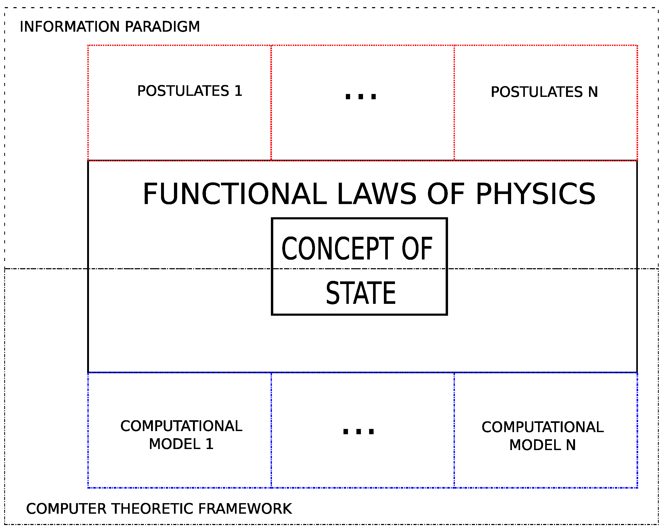
7.1. The Computer-Theoretic Framework: A New Paradigm for Fundamental Physics

When we assume the principle of computability, theoretical computer science appears as a mathematical framework to formulate and discuss theories of fundamental physics. When both elements are combined, a paradigm emerges for the formulation of fundamental physics theories that we have named the computer-theoretic framework (CTF). The CTF involves assuming the principle of computability, using the mathematical framework of theoretical computer science, and giving a physical meaning to its mathematical concepts. In the CTF, a theory to describe the machinery that rules the universe is a computational model, but we address this later on in the paper.
Frameworks are a key element in physics that allow for formulating different theories for a phenomenon. For example, quantum physics [288] and gravitation [289] have been addressed by using frameworks. They also allow us to carry out theoretical calculations to see how the universe would be if the laws of physics were different [290]. A framework defines a set of theories in which the task is finding the theory that better describes the researched phenomena.
Including computational power and computational complexity hierarchy as physical fundamental constants implies a paradigm shift in our view of the universe, and a paradigm shift involves new theories that completely replace the previous ones because the previous paradigm’s concepts are completely substituted by new ones. A reader might therefore ask how accepting the CTF would affect the standard theories of physics. The answer is that the CTF does not conflict with standard theories of physics for two reasons. First, the CTF does not demolish the current paradigms for developing fundamental theories of physics but expands them; it does not propose that computational power and computational complexity hierarchy must substitute other fundamental physical constants but instead adds them to the list of fundamental physical constants. Second, as explained in Section 7, each physical theory can be interpreted as a set of computational functions from a computational space. Thus, all standard theories can be interpreted as computational theories. For example, let us imagine we want to address in the CTF some physical phenomena that require the special theory of relativity. We only need to add the two postulates of the special theory of relativity to the principle of computability because, in set theory, one way to describe a set is stating the properties that its members must satisfy. Therefore, the list of the three statements describes the set of computational models that can explain special relativity. In this kind of definition, the principles or laws of the theory that is combined with the principle of computability function as a filter so that only those computational models whose transition functions fulfil the principles’ or laws’ stipulations belong to the set.
In this way, all physical theories that have been developed until now could be located in this paradigm just by providing a computational interpretation of them. For example, Toffoli provided a computational interpretation of the variational principles [229], so variational principles can be grounded on the principle of computability. To those who wonder what difference this makes, we say that the importance lies in the interpretation of the results obtained when a theory is studied computationally. From the non-computational view, the results of computationally studying a theory are totally independent of the phenomenon because the theory is only a mathematical method to obtain predictions. However, under the CTF, there are two kinds of theories: predictive and descriptive. Predictive theories do not describe the phenomena because the computational features are different from the physical phenomena. Descriptive theories are a precise description of the physical phenomena because the computational features of the theory are considered physical features that the physical phenomena possess. Thus, in the CTF, the computational features of the theory determine what kind of theory it is.
According to these reasons, the paradigm shift that the CTF involves is not the known kind of paradigm shift in which new theories completely replace the previous ones. The paradigm shift that the CTF involves consists only of incorporating new concepts to achieve a more complete description of the universe and adding a computational dimension to existing ones. Also, the paradigm shift that the CTF implies provides a context in which ideas that seem under the current paradigm are merely a random mathematical coincidence, such as the discovery that error-correcting codes are related to supersymmetry [276,291], but those ideas take on a whole new dimension because they cease to be a mere mathematical coincidence and can be interpreted with a physical meaning. Thus, whereas the current paradigm in fundamental physics allows us to understand that the fundamental physical constants associated with our universe's laws of physics must have a specific value to make the life we know emerge, the CTF raises the possibility that certain computational features might also be necessary for a universe to have the laws of physics that allow the kind of life we know.
Considering the previous fact, one may also ask whether the CTF is just a reformulation of standard physics in a computational language without any new contributions. The answer is that it is not a reformulation because the CTF proposes that the computational power and a specific computational complexity hierarchy are physical properties of the universe, requiring their values to be considered in the verification of the theories and therefore studied experimentally. In other words, a theory about a physical phenomenon not only predicts a future state it generates but also describes the computational features of the physical phenomenon. Thus, under the CTF there must be a coherence between the computational power associated with the theory of a physical phenomenon and the computational power that we can find experimentally in the universe. In addition, there must be a coherence between the computational complexity associated with the theory of the physical process and the computational complexity hierarchy associated with our universe. These requirements emerge directly from assuming the principle of computability. Therefore, a theory about a physical phenomenon that does not fulfil those requirements, even when correctly calculating the future state of the physical system, cannot be accepted as a correct explanation of the physical phenomenon.
An important feature that the CTF provides is a way to confront theories of fundamental physics. In the CTF, enunciating a theory about the universe proposes a computational model as the description of the machinery that rules how the universe evolves. We know that two computational models can calculate the same function or even the same set of functions because they have the same computational power. Can we distinguish between two computational models which one better describes the machinery of the universe? Yes, we should be able to make predictions that can be tested. We know that two computational models are equivalent when they have the same computational power, and we also know that two equivalent models can each simulate the operations of the other. This feature allows the existence of virtual machines in the field of operating systems and computers with different architectures that execute the same programs. The execution of a program in a virtual machine entails an increment in the quantity of time of the execution.12 Therefore, we could know whether one computational model versus another is the real machine that rules our universe because the computational steps of the real machine have shorter durations than those of any virtual machine’s steps. If we are given a computational model in which one operation is fundamental and determines the minimum steps, and we find another process that lasts fewer steps than the previous, it shows that the computational model is not the machinery that rules the universe but instead a virtual machine. Thus, we should go deep into the hierarchy of machines to find the physical machine. It should also be taken into consideration that the experiments could show that neither of the computational models has a shorter duration than the other, which would be interpreted to mean that both are virtual machines of the same level, and we should look for a more fundamental machine. Certainly, designing an experiment that uses the hierarchy of machines is a challenge because, although the concept of the hierarchy of machines is very common in the development of commercial software, it involves resolving hard questions about the hierarchy of machines and fundamental physics. For example, it would require knowing the relation between a computational step of the computational models and the fundamental period of time, and the fundamental period of time is still a question being researched [292]. Additionally, with the exception of the theorems about universal Turing machines’ efficiency in simulating Turing machines [133] and their configurations [293], we only have a few results about the process of how asynchronous and synchronous computational systems can execute other machines [294,295,296]. However, even despite the complexity of this approach to confronting fundamental theories, it is an innovative proposal that emerges from the unique point of view that the CTC provides, and if it were developed, it would bring important insights into our understanding of the universe.

7.2. The CTF and Its Formal Formulation

At this point, the reader could be thinking how the principle of computability must be understood and what structure has the paradigm that emerges from it. The answer to this question is that the principle of computability causes a paradigm to emerge because it determines two equations that must be resolved for each physical theory to have a more complete description of the phenomena and our universe. The two equations that emerge are the following:
σ p = P ( T p )
H p = H ( T p )
Equation (1) emerges from the reasoning that if the universe is a computational device, then each physical phenomenon has an associated computational power. Therefore, the equation determines that the computational power σ p that the physical phenomena p possess must be calculated using the theory proposed for the phenomenon, T p . If T p is a theory of everything, σ p will be the computational power predicted by the theory T p for the universe, and therefore, σ p should be a limit for all computational processes that can exist in the universe. This equation presents the challenges of determining the set of values that σ p takes on and defining the function P . The set of values for σ p could be the set of Turing degrees (or degrees of unsolvability) [297]. Regarding function P , it is a challenging topic because we are still researching how to calculate the computational power for a classical computational model [298], and calculating the computational power of a phenomenon using its theory is a process far from standard, as has been shown for the phenomenon of gravity in the field of relativistic computers.
As concerns Equation (2), it emerges from the reasoning that if the universe is a computational device, then each physical phenomenon has an associated computational complexity hierarchy, so the equation determines that the computational complexity hierarchy H p associated with the physical phenomena p must be calculated using the theory proposed for the phenomenon. If T p is a theory of everything, H p will be the computational complexity hierarchy predicted by T p for the universe.
This equation is even more challenging than the previous one because a computational complexity hierarchy can be considered for each computational resource that can be analyzed in the physical phenomena, and so, a priori, we would need one for each computational resource r available in the set of computational resources R ( T p ) . Thus,
H p = r R ( T p ) H p r = r R ( T p ) H r ( T p ) = H ( T p )
It must be noted in Equation (3) that if there were equality relations among the complexity classes of different computational resources, we would need only the computational complexity hierarchy of one computational resource to characterize this aspect of the universe. However, although we know there are relations among complexity classes from different computational resources, many important claims about this topic are only conjectures. Additionally, we only know of two kinds of elements in the set of values that H p can take on: the classical complexity hierarchies and the quantum complexity hierarchies. Moreover, we do not even know whether P = N P [133].
Perhaps while reading the above sections and subsections of this article in favour of the CTF and its computational view, some readers could have the erroneous impression that the CTF is a book of answers for fundamental physics. It is quite the opposite, however, because it brings with it new challenges, as the reader has been able to note in this subsection that theoretical computer science is a field full of important open questions.

7.3. The Scientific Status of the CTF

One question that could be intriguing to the reader is whether or not the CTF has a scientific status due to how wide the paradigm is. The answer is that CTF has a scientific status, and we are going to address this issue here because although the scientific status of a theory is something widely studied, the scientific status of a paradigm has been much less discussed.
The first issue the reader should note is that the principle of computability states that two new fundamental physical constants must be used to describe the universe. That is, the concept of computation must be considered as fundamental as the concepts of energy and spacetime in physics. The second issue is that claiming the existence of a fundamental physical property establishes a paradigm and not a theory. The paradigm determines what shape the theories must have, but it does not establish a quantitative claim that can be contradicted by an observation statement. Third, establishing the fundamental physical property always takes a long time, as with the concept of energy, for example [299,300]. Even the concept of space, which could be considered an immediate concept because of our school education, required humans to do a lot of conceptualisation and abstraction [301]. The principle of computability is the consequence of almost a century of research work by brilliant scientists.
With the above three points in mind, we now look at how to determine whether a paradigm has a scientific status. From the point of view of conceptualization, a fundamental physical property is a fundamental concept in the framework that emerges from it. A framework’s fundamental concepts are independent of each other because the rest of the concepts emerge from the combination of them. Scientifically evaluating a paradigm involves testing the independence of the fundamental concepts. For example, Minkowski contributed to building a new paradigm proposing the fundamental concept of spacetime when Einstein’s theory required replacing the Newtonian paradigm and its concepts of space and time because of the understanding the constancy of the velocity of light [302].
The complexity of establishing the scientific status of a paradigm emerges from the fundamental concepts not being easily falsifiable because it involves thinking of an experiment that shows that all possible instances of the concept are wrong. Thus, devising an experiment to test a paradigm is much more difficult than devising an experiment to test a theory. In addition, because a paradigm is a tool that we use to think about the theories that describe the world, devising such experiments would involve our ability to produce an alternative fundamental concept to substitute those in the paradigm that want to be tested. For example, can the reader imagine an experiment to test the concept of energy and the paradigm that emerges from it? Fortunately, another criterion can be used to determine the scientific status of a paradigm, and this criterion is related to the theories elaborated in the paradigm. If the theories formulated in a paradigm are falsifiable, the paradigm has a scientific status. Regarding the CTC, any theory formulated makes two predictions: assigning one specific computational power and assigning one specific computational complexity hierarchy to the universe. These two predictions could be contradicted by an empirical test which implies directly that all the theories formulated in the CTF are falsifiable. For example, the prediction about the computational power could be proven false if a computational device were built that overcame the computational power assigned to the universe. The prediction about the computational complexity hierarchy could be proven false if a computational device were also built that executed a process to resolve a problem in a complexity class different from that assigned by the computational complexity hierarchy designated by the theory. According to the criterion mentioned and the fact that all the theories formulated in the CTF are falsifiable, the CTF has a scientific status.

7.4. Developing Theories of Fundamental Physics in the Computer-Theoretic Framework

The principle of computability speaks about computational power and computational complexity hierarchy as two fundamental physical constants that characterise our universe, so it must be noted that we could know the computational power and the computational complexity of the universe, but knowing both values does not tell us what kind of computational system our universe is. Although just knowing these values would be of significant value for developing a quantum theory of gravity because of the reasons Geroch and Harle explained [285], the main objective that emerges in the CTF is determining what kind of computational system the universe is. Doing so means determining what computational model describes it, so stating a fundamental theory of physics in the CTF is proposing a computational model. In the scientific literature, examples of this kind of research can be found. We already mentioned Calude et al.’s work addressing the complementarity of quantum mechanics [240,241], which is an important issue in modern physics [303]. We have also spoken about ’t Hooft’s work that attempts to describe quantum field theory using CA [57].
We think that the approach of using a computational model as a theory could be very useful for fundamental physics. For example, many issues could be researched using computational models, such as the problems of consistency discovered in quantum mechanics [304,305] and its solutions [306], the measurement problem [243], and the problem of the Copenhagen interpretation assigning a state of the universe [307,308]. The computational model we think could help in this research is the quantum game of life [309,310,311,312]. We make this claim based on the fact that, as in the classical Conway’s Game of Life, it seems that structures also emerge in the quantum game of life [313]. Thus, if we find structures that emerge in the quantum game of life and share information, studying those processes could help to understand or reveal key issues to resolve the problems mentioned.
Although we have suggested the quantum game of life for researching some topics, determining a computational model to enunciate a fundamental theory of physics is a complex endeavour. We want to show this complexity, but before we do, we need to explain what a computational model is. A computational model has three kinds of elements: the units of computing, the alphabets, and the rules of computation. We propose the following definitions of a computational model.
  • Units of computing. The units of computing are the elements that contain the information that defines the system’s state. A computational model can have different kinds of units of computing.
  • Alphabets. Each alphabet is associated with one kind or several kinds of units of computing, which means that each element of an alphabet is a value that can be contained by a unit of computing of the kind associated with that alphabet.
  • Rules of computation. The rules of computation determine how the value that contains each unit of computing changes.
When considering a computational model to be a fundamental theory of physics, the data contained in the units of stating would be what Ilachinski has called “primordial information” [54] (p. 634).
Initially, one could think that the definition of a computational model is too simple to address the development of a fundamental theory of physics. However, labelling the definition as simple would be misleading because it is general, not simple. We know this definition is general because it allows many different lines of research, and these possibilities make the research in the CTF very complex. To understand the level of complexity of determining a computational model to describe the universe, the following overview presents different research paths that must be taken into account a priori to find that computational model.
On the basis of the definition of a computational model that we have given, we show below several research paths that could be followed to develop fundamental theories in the CTF. One of the major issues that divides the research emerges from the conceptualization of space in the computational models, so we have the two following research paths:
  • The units of computing are space. This line of research considers space as the fundamental machinery, so each unit of stating is a position of space. Both CA and QCA are examples of computational models in this line of research.
  • In a computational model, the units of computing are an underlayer when they store both the particles and their spatial locations. If the units of computing are an underlayer, they cannot be identified with spatial locations. A computational model in which the units of computing are an underlayer could execute declarative programs perceived as a universe ruled by the principle of least action. Research on the holographic principle would be in this line of research.
Each of these research paths can be divided by considering the cardinality of the alphabets in the computational model. We have computational models with the following cardinalities:
  • Finite computational models. The units of computing are a finite number, and all alphabets of the computational model have a finite number of elements.
  • Countable infinite computational models. The number of the units of computing is a countable infinite number, and all alphabets of the computational model have a countable infinite number of elements.
  • Uncountable infinite computational models. The number of the units of computing is an uncountable infinite number, and all alphabets of the computational model have an uncountable infinite number of elements.
  • Hybrid computational models. The alphabets and the units of the computational model can have different cardinalities.
The research can also be divided by considering the feature of synchronicity in the units of computing. Doing so produces the following lines of research:
  • Synchronous units of computing. The computational model has a global synchronous update signal.
  • Asynchronous units of computing. The computational model does not have a global synchronous update signal, so the units of computing update their values independently of what the other units of computing do.
The last way in which the previous lines of research can be divided is by considering a feature of probability in the rules of computation.
  • Probabilistic rules of computation. The rules of computation determine how likely an element of an alphabet will be contained by the unit of stating when the units of computing update their values.
  • Deterministic rules of computation. The rules of computation determine one specific value that will be contained by the units of computing when they update their values.
Considering only the possibilities of the features mentioned, we have obtained 64 lines of research. However, we could consider even more features, such as a static or dynamic number of units of computing that would generate different kinds of computational models. In addition, considering whether the rules of computing do or do not fulfil locality generates different research paths, as was mentioned in the discussion about QCA. Moreover, the computational model of the universe could be a hybrid computational model as the result of several computational models coupled either in a manner similar to the construction that occurs in coupled cellular automata [314] or in any other kind of coupling that we have not even imagined yet.
It is important to note that in the CTF, when assuming a property is a fundamental physical property of the universe rather than another (e.g. discrete vs continuous), one kind of computational model is chosen to research. In addition, although we have an important list of different types of computational models, it does not mean that we have already formulated the type of computational model that describes the machinery of the universe. For example, Wolfram has recently presented a new type of computational model based on graphs and hypergraphs [315]. Thus, the complexity of research in the CTF emerges not only because theoretical computer science is a field full of open questions but also because of the huge landscape of computational models and the little information available to select which model to research.

8. Discussion

In the previous section, we introduced the CTF, a paradigm that uses concepts of theoretical computer science to address the development of fundamental theories of physics. While the information-theoretic paradigm has been used explicitly since information theory emerged [233] and is widely accepted in physics in the field of thermodynamics [12,13], computational models have been considered second rate in the world of physics [1,5]. Until now, computational concepts have been used in physics without an explicit paradigm that provides a context for interpreting results and possible directions. We have proposed a new paradigm, the CTF, that determines the need to incorporate computational concepts when discussing natural phenomena, and the principle of computability is its basis because this principle determines that a computational power value and a computational complexity hierarchy must be included in the description of the universe and that these values must be interpreted as fundamental physical constants of the universe. Therefore, the computational power and the computational complexity hierarchy associated with each physical theory of a physical phenomenon are also part of the description that the physical theory makes of a physical phenomenon. We have also pointed out that the term computational system in the formulation of this new principle must not be identified as any digital computational model; its meaning is more general and does not reference any specific kind of computational model. A paradigm for formulating and interpreting theories of fundamental physics does not affect only fundamental physics, because physics is the basis for the rest of the sciences, so the view and formulation of the CTF affects different issues, and we are going to discuss several of them below.

8.1. Researching the Computability of the Universe

The classical view on physics and computation is that physical processes allow computational processes when a computational process is a calculus with numbers [42]. The views Rosen and Zuse proposed on the relationship between physics and computation were so revolutionary that the scientific community did not pay attention to them until several decades later. Shifting to this new view can be compared to that which happened with geometry in the 19th century, when Gauss and Riemann proposed that geometry is a physical property and should be determined with experimental research. Initially, Euclidean geometry was thought to be the only possible geometry for space. However, we later understood that other geometries exist that generate other geometrical spaces which, from a mathematical point of view, are also correct. The modification of Euclid’s fifth postulate determines other geometries, and in computation, the modification of the domain, codomain, and list of limitations determines different computational spaces. In the same way that geometry is a feature of our universe, we claim that computational power and the computational complexity hierarchy are physical properties and must be studied through experimental research.
As we have seen in Section 4, several researchers have made claims against the idea that the universe is a computational system, arguing that non-computational physical phenomena exist. We also explained that the term non-computational (or uncomputability) cannot be used in absolute terms; it needs to reference a computational model which determines a computational space. Since the computational power of our technology is limited to the computational space generated by a Turing machine, we usually omit the computational model, but we must always be aware that the notions of computational and non-computational are not absolutes. In addition to that misunderstanding, there is a misconception regarding the issue of the existence of non-computational physics. The claim that some issues are non-computational does not mean that the phenomenon is not carried out by a computational system but that we have a limitation in our capability to predict the evolution of the phenomenon. Wolfram has already provided a physical interpretation of non-computational physical processes using the concept of computational irreducibility, but it is worth discussing this issue to clarify the matter as much as possible. To address this issue, we can turn to the halting problem, which is the problem of achieving an algorithm capable of determining whether an arbitrary Turing machine will terminate or run forever. Turing proved that there is no Turing machine that can solve the halting problem [21]. Nevertheless, we must not overlook the fact that the arbitrary Turing machine for which we want to know whether it will terminate can be defined without any problem—the issue is that we cannot calculate whether the Turing machine is going to terminate before it happens. Similarly, when it is proven that a physical system is non-computational, it means that there is no algorithm that can be implemented in a Turing machine that calculates an answer to any physical question about the future state of the system only using the initial configuration. Therefore, the existence of non-computational physics does not invalidate the principle of computability because it does not imply that there is a physical system in nature indescribable by any computational model. Non-computational physics only means that limits exist to create general methods that directly calculate the future state of some kinds of physical systems from the initial state.
The CTF proposes that the way to understand the mechanism that rules the universe is to identify it as a computational model. This is not as strange of a proposal as one might initially think because Dirac already showed us that we need to go beyond the numbers to understand the deep aspects of the rules of the universe, which is a process that requires complex mathematical objects [316]. This way of thinking continues today. For example, recently, a group of physicists led by Pierpaolo Mastrolia and Sebastian Mizera have revealed an underlying mathematical structure in the equations of particle collisions that involve the intersection numbers [317,318]. Another example is the Bell-like experiment just proposed [319] and the experiments being carried out [320,321] to determine whether the mathematical structure underlying complex numbers is more relevant than real numbers in describing the quantum world. Therefore, looking for a computational model is nothing but following the path Dirac started because a computational model is merely a complex mathematical object.
For the reasons that we explained in Section 7, when a computational model is proposed as a theory of fundamental physics in the CTF, its fundamental elements are bound to specific physical entities because it is a description at the level of fundamental physics. Regarding this fact, the CTF’s context is completely different from computer engineering’s because the computational model in computer engineering is built within a physical level that has physical sublevels. Therefore, if a computational model is proposed in the CTF, it is enunciating the fundamental entities and causalities of our universe.
According to what was explained in Section 7.2, assuming the CTF makes the following two objectives appear in the field of physics:
  • Physics must determine what computational class the universe belongs to.
  • Physics must determine what computational model the universe is.
Regarding the first objective, determining the computational class of the universe means that at least the two new fundamental physical constants stated in the principle of computability should be determined. Although most researchers are not working with that goal in mind, the research toward achieving quantum computation and other types of computation will shed light on which computational class our universe belongs to. Understanding this will allow us to know if the Tegmark–Szudzik thesis is true. If hypercomputation exists, the Tegmark–Szudzik thesis and the physical Church–Turing principle are false. In addition, it is important to note that the Tegmark–Szudzik thesis does not involve the Zuse–Fredkin thesis because the Tegmark–Szudzik thesis does not propose one specific mechanism that rules the evolution of the universe; it is only a presumed feature of the mechanism. However, the Zuse–Fredkin thesis does involve the Tegmark–Szudzik thesis because the cellular automaton model does not exceed the Church–Turing limit.
It must be noted that the Tegmark–Szudzik thesis is connected to the search for a theory of everything (TOE). If the Tegmark–Szudzik thesis is true, then the Church–Turing limit in computational power is a criterion for searching for a TOE. We can observe this in classical mechanics. We know from physical experiments that classical mechanics is not a TOE because the quantum world and high gravity systems cannot be explained by classical mechanics. In the CTF, we obtain the same conclusion: if the Tegmark–Szudzik thesis is true, classical mechanics cannot exceed the Church–Turing limit. However, different theoretical studies show that classical physics is beyond the Church–Turing limit. For example, regarding the wave equation, we know it is not Turing computable [322,323], and the results of computational analysis also show undecidability and incompleteness in classical mechanics [324]. Therefore, if the Tegmark–Szudzik thesis is true, classical mechanics cannot be a TOE because classical mechanics predicts physical objects capable of calculations beyond the Church–Turing limit, contradicting the Tegmark–Szudzik thesis. Figure 1 shows the relationships between the different claims about the computational features of the universe.
More challenging than the first objective is the second, because determining the computational model that describes which computational system our universe is requires knowing many fundamental physical features that physicists have been trying to determine for a long time. For example, to know which computational model to follow in research—the one that considers spacetime discrete or the one that considers it continuous—the nature of spacetime should be determined experimentally. Thus, experiments to determine the nature of spacetime [255,325] are fundamental to advancing the search for which class of computational model the universe belongs to. Another example is distinguishing between the research lines of CA and QCA. The perspectives of CA and QCA differ deeply in the kind of universe they propose, but to the best of our knowledge, we do not know of even one experiment that can differentiate one from the other. Assuming ’t Hooft’s hypothesis [58,60], the vacuum of CA and QCA should be different because the empty space of his computational models contains information, and every empty space of the universe can diverge. Given that this topic is outside our field, we cannot imagine an experiment to test this difference, but we have mentioned it to stimulate research on the issue.

8.2. Information and Computation

In many papers, the concepts of information and computation are mentioned together as if these two concepts were of the same paradigm. However, a different paradigm emerges from each one: the information paradigm and the CTF. These paradigms are complementary because information and computation are closely related to the concept of state; however, they are disjointed in that they address different issues with regard to the concept of state. For example, when a physical theory is studied within the CTF, the objective is knowing the computational power associated with it, whereas within the information paradigm, the objective is knowing the quantity of information the physical laws contain [326]. We already explained in Section 3 why the concept of state is important in computation, but it is worthwhile to examine why there is a close relationship among state, physics, and information. The reason resides in the fact that the theory of information establishes that the concept of state is fundamental to knowing the quantity of information because that quantity is related directly to the number of different possible states in which a system can be. Thus, a physical system whose number of possible states is greater than the number of states of another contains a quantity of information greater than the physical system with a lesser number of states. It is important to note that the quantity of information assigned to a state depends on the kind of state, so, for instance, the quantity of information stored in a classical state is different from that stored in a quantum state.
By clarifying these issues, we can better understand what can be done in each paradigm. In the case of the information paradigm, it can be used to formulate informational principles, and one can study which physical theories fulfil them [327]. Additionally, it can be also used to find a set of informational principles from which quantum theory is derived [328,329]. However, when the CTF is used to research a theory, one does not look for a set of informational principles but a computational model that describes how the physical system’s state evolves. In other words, while the information paradigm poses the problem of looking for a set of fundamental principles about the quantity of information from which the theory derives, the CTF poses the problem of finding the machinery under the theory. Figure 2 describes graphically the relationship between the information paradigm and the CTF.

8.3. Is the CTF Proposing Platonic Realism?

Tegmark connects the Tegmark–Szudzik thesis with the MUH [198], which has been interpreted as a defence of Platonist realism [330]. Given that the MUH claims that the universe is a mathematical structure and the CTF accords with that hypothesis because a computational model is a mathematical structure, one could ask whether the CTF contains a Platonic realism view of the universe. However, we do not interpret that the MUH claims that mathematics is the ultimate substance of the universe. Different views exist in the philosophy of mathematics: Platonism, semi-Platonism, Aristotelianism, and nominalism [331]. The Platonic view that mathematics is an external reality is far from our interpretation. We also disagree with the nominalistic view, which negates the existence of mathematical universals. Our view fits with Aristotelian realism, which proposes that mathematical objects do not exist in a separate world but are embodied in the material world [332]. In other words, Aristotelian realism proposes that mathematics emerges from the physical world through studying the relations of physical objects. Our brains are able to perceive and recognise the patterns of the parts of complex physical objects and build the language of mathematics on the basis of these patterns. When we interpret the MUH, we understand that the universe contains elements that behave with a regularity that can be described with the language of mathematics. Hence, we do not interpret the MUH and the CTF as defences of Platonic realism but as mathematical defences of physicalism because our interpretation denies the existence of mystic mathematical objects in a different reality connected with our universe.

8.4. The CTF and the Unreasonable Effectiveness of Mathematics

Since Eugene Wigner wrote his famous article about the unreasonable effectiveness of mathematics in the natural sciences [333], this conundrum has continued to this day. To solve this problem, Penrose proposed the triangle Matter–Mind–Math by describing the three relations among these elements [121]. However, some defend the existence of these relations and others criticise it [334]. The triangle Matter–Mind–Math expresses that matter embodies mathematics among other ideas. Those defending this idea do so on the fact that considering our universe to be intrinsically mathematical has led to many achievements; the physical world must therefore be isomorphic to any mathematical structure [198,334]. Yet, that justification does not explain how human beings can do calculations to describe a physical system radically different from them, such as a Bose–Einstein condensate. Assuming the CTF, however, sheds light on the conundrum exposed by Wigner. If the universe is a computational system, regardless of the kind of computational system, we are also part of the computations carried out by that computational system. The computability theory shows that two computational models, even those having very different structures or characters, can simulate each other or themselves if they have the same computational power. For example, a Turing machine can simulate a register machine, and universal Turing machines that can simulate any arbitrary Turing machine exist. Additionally, of course, a more powerful computational model can reproduce the calculations that a less powerful computational model carries out. Thus, the CTF explains that the effectiveness of mathematics in the natural sciences is a consequence of the fact that a computational model can simulate the computations of a different computational model. Evidence in favour of the CTF’s explanation for the unreasonable effectiveness of mathematics is the proof that Conway’s Game of Life possesses the capacity of universal computation [335]. The proof consists in building a Turing machine using different structures simpler than a Turing machine that the rules of Conway’s Game of Life allow to appear. Even though Conway’s Game of Life is a cellular automaton, a Turing machine structure can emerge in it because it is able to do universal computation. Thus, although the cellular automaton is different from a Turing machine, the mathematical concept of the Turing machine appears in Conway’s Game of Life from the Turing machine structure that emerges in the cellular automaton.

8.5. Cognitive Behaviour and Physics

From a physicalist position, physics must provide a basis for every natural phenomenon [336]. Although physics provides the foundation for chemistry and biology, it is under discussion whether physics provides a basis for the behaviour of living beings, which is one of the more natural phenomena. There have been some proposals to include the phenomenon of behaviour in physical theories [337], but the most successful theories that describe and predict behaviour have not been related to fundamental physics. Cognitive science, which was born in the 1950s, contains the most fruitful theories to explain many kinds of human behaviours [338], and it proposes that the mind is a computational process carried out by the brain. In his famous book Computation and Cognition, Zenon Pylyshyn proposed and defended that the claim that mental processing is computational is not a metaphor but a real fact [339]. Since then, a large majority of the cognitive science community consider a cognitive process to be a computational process. However, they also claim that a computational process is not a physical process. For example, Pylyshyn stated the following:
“In chapters 1 through 5, I spoke of the independence of the physical and computational, or symbolic, descriptions of a process” [339] (p. 149).
“By mapping certain classes of physical states of the environment into computationally relevant states of a device, the transducer performs a rather special conversion: converting computationally arbitrary physical events into computational events” [339] (p. 152).
By considering Pylyshyn’s ideas, we see that cognitive scientists hold the view that the computational theories of cognitive science are isolated from physics.
The current relationship between physics and cognitive science is problematic if we aspire to achieve one complete explanation of our universe. We see it as extremely difficult that any technology will allow predicting macroscopic behaviours of human beings using the fundamental laws of physics due to the huge number of calculations required. However, we can obtain this explanation if physics provides a fundamental concept linked to the basis of cognitive science, and we believe that the CTF opens the door to this link. Pylyshyn’s view differentiating physical and computational processes is based on the view that ignores the possibility that the universe is a computational system. However, the CTF assumes a computational view of the universe that provides a direct link between physics and cognitive science, opening the door to considering physics as the basis of the theories formulated by cognitive science until now. The connection emerges from the fact that the computational power of two different computational models can be evaluated by comparing the sets of functions or the sets of algorithms they can carry out. Each of the functions, or algorithms, of the set is encoded in the machinery of the computational model, and the process the computational model performs to calculate the function is obviously a computational process. Thus, assuming the principle of computability, the universe is a computational system and physical processes are computational processes, and they encode functions and algorithms. This conclusion opens a path to connecting the basis of computational cognitive science with physics.
Another issue that concerns the fields of physics, computer science, and cognitive science under the CTF is the proposal that the mind is a hypercomputational process [340,341]. The most extended scientific view of the mind considers it to be a functional state of the brain [342], so it is a physical process of a physical system. Thus, assuming the principle of computability, the mind could be only a hypercomputational process if the universe’s machinery allows hypercomputational processes, which in turn implies that the Tegmark–Szudzik thesis and the physical Church–Turing principle are false.

9. Conclusions

This article addresses different issues regarding the relationship between physics and theoretical computer science. We reviewed how computer-theoretic concepts have penetrated the field of physics. This has happened to such an extent that it has been proposed that the universe is a computer. Having examined this rapid diffusion of computational concepts in physics, we showed that it did not happen by chance but because physics and computation are deeply connected due to the concept of state. We also introduced the concept of computational space, which we consider useful for understanding different issues to deal with the computational description of nature. The first issue we addressed is the debate about the claim that the universe is a computational system; because this claim has been criticised, we reviewed and analysed several of these arguments against the claim that the universe is a computational system that we found in the literature. We showed that these arguments are not valid because they make the same mistake: they identify a computational system with one specific type of computational model, overlooking that many different computational spaces exist, each of which allows different kinds of computational models. Church and Turing found a computational limit in a specific computational space, but that finding was only the beginning of the field of theoretical computer science.
The next issue we analysed is Edis and Boundry’s proposal to solve Hempel’s dilemma using computational theory. Contrary to what they stated, we find no reason to accept that an oracle would not be a natural object if one were found. The fact that our conscious process of thinking is a finite, sequential process does not imply that a system more computationally powerful than a Turing machine would be supernatural. Applying Occam’s razor, we should not multiply entities formulating natural and supernatural entities if we found a meaningful oracle. Instead, we would have to consider that fact as proof that one or more wrong assumptions about nature exist and that oracles exist in our universe.
Another issue we reviewed is whether our universe is a computational simulation. We have determined that this claim and the claim that the universe is a computational system are stating two different facts. The first asserts that a programmable computational system executing the simulation exists, whereas the second determines only that a computational system that exists and does not involve our being is part of a simulation running in a computational system.
Analysing these issues has led us to realise that the claim that the universe is a computational system can be formulated as a principle from which emerges a new scientific paradigm that uses theoretical computer science concepts to formulate fundamental theories of physics. We have named it the computer-theoretic framework (CTF). After reviewing the literature, one can see that many ideas of the CTF have been implicit in the works of different physicists for several decades. Thus, the formulation of the CTF synthesises and integrates these ideas and shows them explicitly. The mainstay of the CTF is the principle of computability, the claim that the universe is a computational system, but this principle does not determine one specific computational model and space. Thus, the principle of computability requires physics to find the computational model and space that describe and explain the universe.
One important issue to note is that although the claim that the universe is a computer sounds radical, the CTF does not provide a new radical view about the concept of physical phenomena or the universe but a deeper and more precise view of what a physical phenomenon is and what describes its mathematical theory. This kind of deep understanding already happened in mathematics when computability theory emerged. This theory changed our view about calculations in mathematics, and its results have allowed us to understand that an advanced skill in performing operations is not enough to carry out some calculations, as limits exist that cannot be overcome with any level of skill [22]. Furthermore, let us remember that Wheeler pointed us toward Era III of physics, in which “...we have to seek nothing less than the foundation of physical law itself” [343] (p. 121). The CTF is a scientific paradigm to carry out that search, as it is not a proposal to generate new theories in fundamental physics and replace the current ones but to expand and investigate them by seeking the foundation of physical law itself in the form of a computational system.
Finally, we have discussed how the CTF’s new view on computation and the physical phenomenon affect fundamental physics and the CTF’s relationship to mathematics and the basis of cognitive science.
From the analysis and discussions carried out in this article, we conclude with the two following statements:
  • A scientific paradigm exists, called the CTF, to develop fundamental theories of physics based on the concepts of theoretical computer science.
  • The CTF highlights computational power and the computational complexity hierarchy as fundamental physical constants of the universe.
In summary, we think there are important arguments that indicate that computational power and the computational complexity hierarchy should be considered fundamental physical constants that describe the universe, and that the CTF provides a coherent interpretation that integrates them with the rest of the known fundamental physical constants to supply a description of the universe. Thus, computer science and fundamental physics can propel each other forward, as geometry and physics have already done. However, understanding the computational aspects of the universe will be difficult if foundations and scientific organisations do not create specific programs that promote fundamental physics research by applying the view proposed by the CTF because most scientists within the fields of computer science and fundamental physics are unfamiliar with the other field. We are aware that creating ambitious programs that require multidisciplinary research is not easy, but it would not be the first time a massive effort was carried out to develop a new scientific area. For example, in the 1970s, important foundations and national programs encouraged the development of cognitive science by promoting collaboration among scientists within psychology, neuroscience, linguistics, philosophy, and artificial intelligence. We believe that the CTF is the road to the future of fundamental physics, but we are also aware that without programs that encourage training in physics and theoretical computer science and collaboration between those working in these two fields, this road will remain closed.

Author Contributions

This article is based on one section of a chapter of S.M.-T.’s PhD thesis [344]. All the concepts and ideas proposed in this paper have been conceived by S.M.-T. The principle of computability, its formulation, and its consequences have been conceived by S.M.-T. S.M.-T. has written the article. Á.L.S.-L. and L.A.-R. have read and reviewed the article. All authors have read and agreed to the published version of the manuscript.

Funding

This research received no external funding.

Institutional Review Board Statement

Not applicable.

Informed Consent Statement

Not applicable.

Data Availability Statement

Not applicable.

Acknowledgments

Sergio Miguel-Tomé would like to thank Luis Alonso-Romero and Ángel Luis Sánchez-Lázaro for agreeing to supervise his doctoral thesis, allowing him to research the topic that mattered most to him, and always defending his work. Without their support, this article would not have been possible. Sergio Miguel-Tomé would also like to thank Moritz Müller, who taught him the foundations of computational complexity theory at the Kurt Gödel Research Center for Mathematical Logic at the University of Vienna with no interest other than sharing knowledge. In the end, this knowledge has been of great value in addressing the topic of this article. The authors are also grateful to Lori-Ann Tuscan for assisting with language editing.

Conflicts of Interest

The authors declare no conflict of interest.

Abbreviations

The following abbreviations are used in this manuscript:
CTCClosed Time-like Curve
CTFComputer-Theoretic Framework
MUHMathematical Universe Hypothesis
PCEPrinciple of Computational Equivalence
CUHComputable Universe Hypothesis
CACellular Automata
QCAQuantum Cellular Automata

Notes

1
A function is implemented when it can generate the correct output when given an input.
2
In his article, Deutsch called this principle the Church–Turing principle, but we consider it more appropriate to use its author’s name because, as we explain in this paper, neither Church nor Turing claimed anything in their original statements about the physical world but about a framework of mathematics, the finitary point of view.
3
Subsequently, a better definition appeared [96].
4
We have not added Deutsch’s name because he has rejected the idea that the universe is a computer in public interviews. Deutsch’s declarations can be checked in the program Closer to Truth, answering the question Is the Cosmos a Computer? [195]
5
The list of selected challenges is on the London Institute for Mathematical Sciences website: https://lims.ac.uk/23-mathematical-challenges/ (accessed on 25 August 2021).
6
To keep this explanation simple, we constrain it to the non-probabilistic formulation, but it could be formulated yet in a more general way using probabilistic functions because a non-probabilistic function can be seen as the particular case of a probabilistic function. The probabilistic function assigns to each element of the domain a subdistribution of elements of the codomain δ : Y [ 0 , 1 ] , so a non-probabilistic function can be seen as the particular case where all the subdistributions assign probability 1 to one of the elements of the codomain and 0 to the others.
7
D = C is permitted.
8
If we were using a probabilistic framework, then the machine would compute a probabilistic function if it generated each output with the same probability as the probabilistic function.
9
The term computational space has not been used in the computability theory, but we consider that introducing this term can make various ideas more understandable and facilitate discussion of them.
10
We assume that Deutsch considers that attribute and property are equivalent.
11
Digital computers are synonymous with discreteness, and they should not be identified as binary technology because it is only one of the possible digital technologies. For example, we could have a ternary technology, which would be a digital technology, and build a ternary computer with it.
12
The increment of time is a constant quantity, so it is assumed to be a minor matter compared with duplicating or triplicating the hardware.

References

  1. Svozil, K. Computational universes. Chaos Solitons Fractals 2005, 25, 845–859. [Google Scholar] [CrossRef] [Green Version]
  2. Zenil, H. FRONT MATTER. In A Computable Universe: Understanding and Exploring Nature as Computation; World Scientific Publishing Company: Singapore, 2013; pp. i–xliv. [Google Scholar]
  3. Lloyd, S. Ultimate physical limits to computation. Nature 2000, 406, 1047–1054. [Google Scholar] [CrossRef] [Green Version]
  4. Lloyd, S. Computational capacity of the universe. Phys. Rev. Lett. 2002, 88, 0110141. [Google Scholar] [CrossRef] [Green Version]
  5. Margolus, N. Looking at Nature as a Computer. Int. J. Theor. Phys. 2003, 42, 309–327. [Google Scholar] [CrossRef]
  6. Cuffaro, M.; Fletcher, S. Introduction. In Physical Perspectives on Computation, Computational Perspectives on Physics; Cambridge University Press: Cambridge, UK, 2018; pp. 1–22. [Google Scholar]
  7. Deutsch, D. What is Computation? (How) Does Nature Compute? In A Computable Universe: Understanding and Exploring Nature as Computation; World Scientific Publishing Company: Singapore, 2012; pp. 551–566. [Google Scholar]
  8. Zenil, H. (Ed.) Irreducibility and Computational Equivalence: 10 Years After Wolfram’s A New Kind of Science; Springer: Berlin/Heidelberg, Germany, 2013. [Google Scholar]
  9. Tong, D. The Unquantum Quantum. Sci. Am. 2012, 307, 46–49. [Google Scholar] [CrossRef] [PubMed]
  10. Wharton, K. The Universe is not a computer. In Questioning the Foundations of Physics; Springer: Berlin/Heidelberg, Germany, 2015; pp. 177–189. [Google Scholar]
  11. Longo, G.; Paul, T. The Mathematics of Computing between Logic and Physics. In Computability in Context: Computation and Logic in the Real World; World Scientific: Singapore, 2009; pp. 243–274. [Google Scholar]
  12. Parrondo, J.; Horowitz, J.; Sagawa, T. Thermodynamics of information. Nat. Phys. 2015, 11, 131–139. [Google Scholar] [CrossRef]
  13. Maruyama, K.; Nori, F.; Vedral, V. Colloquium: The physics of Maxwell’s demon and information. Rev. Mod. Phys. 2009, 81, 1–23. [Google Scholar] [CrossRef] [Green Version]
  14. Fidora, A.; Sierra, C. (Eds.) Ramon Llull: From the Ars Magna to Artificial Intelligence; Consejo Superior de Investigaciones Científicas: Madrid, Spain, 2011. [Google Scholar]
  15. Leibniz, G. Dissertatio de Arte Combinatoria; Sämtliche Schriften und Briefe: Berlin, Germany, 1666. [Google Scholar]
  16. Drake, S. Galileo and the First Mechanical Computing Device. Sci. Am. 1976, 234, 104–113. [Google Scholar] [CrossRef]
  17. Swade, D. Redeeming Charles Babbage’s Mechanical Computer. Sci. Am. 1993, 268, 86–91. [Google Scholar] [CrossRef]
  18. Corry, L. David Hilbert and the Axiomatization of Physics (1898–1918): From Grundlagen der Geometrie to Grundlagen der Physik; Archimedes: New Studies in the History and Philosophy of Science and Technology; Kluwer Academic Publishers: New York, NY, USA, 2004. [Google Scholar]
  19. Hilbert, D. Axiomatisches Denken. Math. Ann. 1918, 78, 405–415. [Google Scholar] [CrossRef]
  20. Gödel, K. Über formal unentscheidbare Sätze der Principia Mathematica und verwandter Systeme I. Monatshefte Math. Phys. 1931, 38, 173–198. [Google Scholar] [CrossRef]
  21. Turing, A.M. On Computable Numbers, with an Application to the Entscheidungsproblem. Proc. Lond. Math. Soc. 1936, s2-42, 230–265. [Google Scholar] [CrossRef]
  22. Davis, M. Computability and Unsolvability; Dover Publications: Mineola, NY, USA, 1982. [Google Scholar]
  23. Sipser, M. Introduction to the Theory of Computation, 3rd ed.; Cengage Learning: Boston, MA, USA, 2012. [Google Scholar]
  24. Papadimitriou, C.H. Computational Complexity; Addison Wesley Longman: Cambridge, MA, USA, 1994. [Google Scholar]
  25. Alhazov, A.; Leporati, A.; Mauri, G.; Porreca, A.E.; Zandron, C. Space complexity equivalence of P systems with active membranes and Turing machines. Theor. Comput. Sci. 2014, 529, 69–81. [Google Scholar] [CrossRef]
  26. Rosen, R. Church’s thesis and its relation to the concept of realizability in biology and physics. Bull. Math. Biophys. 1962, 24, 375–393. [Google Scholar] [CrossRef]
  27. Wiener, N.; Rosenblueth, A. The mathematical formulation of the problem of conduction of impulses in a network of connected excitable elements, specifically in cardiac muscle. Arch. Inst. Cardiol. Méx. 1946, 16, 205–265. [Google Scholar]
  28. Konrad, Z. Rechender Raum. Elektron. Datenverarb. 1967, 8, 336–344. [Google Scholar]
  29. Konrad, Z. Rechender Raum; Friedrich Vieweg & Sohn: Braunschweig, Germany, 1969. [Google Scholar]
  30. Toffoli, T. Cellular Automata Mechanics; Technical Report Tech. Rep. No. 208; The University of Michigan: Ann Arbor, MI, USA, 1977. [Google Scholar]
  31. Toffoli, T. Computation and construction universality of reversible cellular automata. J. Comput. Syst. Sci. 1977, 15, 213–231. [Google Scholar] [CrossRef] [Green Version]
  32. Fredkin, E.; Landauer, R.; Toffoli, T. Physics of Computation. Int. J. Theor. Phys. 1982, 21, 903. [Google Scholar]
  33. Feynman, R. The Character of Physical Law; MIT Press: Cambridge, MA, USA, 1965. [Google Scholar]
  34. Hopfield, J. Feynman and Computation. In Feynman and Computation; Perseus Books Publishing: New York, NY, USA, 1998; pp. 3–6. [Google Scholar]
  35. Wheeler, J. Pregeometry: Motivations and Prospects. In Quantum Theory and Gravitation; Academic Press: Cambridge, MA, USA, 1980; pp. 1–11. [Google Scholar]
  36. Wheeler, J. Information, Physics, Quantum: The Search for Links. In Complexity, Entropy, and the Physics of Information; Addison-Wesley: Boston, MA, USA, 1990; pp. 309–336. [Google Scholar]
  37. Feynman, R. Simulating Physics with Computers. Int. J. Theor. Phys. 1982, 21, 467–488. [Google Scholar] [CrossRef]
  38. Minsky, M. Cellular Vacuum. Int. J. Theor. Phys. 1982, 21, 537–551. [Google Scholar] [CrossRef]
  39. Fredkin, E. Digital Mechanics. Physica D 1990, 45, 254–270. [Google Scholar] [CrossRef]
  40. Mainzer, K.; Chua, L. The Universe as Automaton: From Simplicity and Symmetry to Complexity; Springer: Berlin/Heidelberg, Germany, 2012. [Google Scholar]
  41. Fredkin, E.; Toffoli, T. Conservative logic. Int. J. Theor. Phys. 1982, 21, 219–253. [Google Scholar] [CrossRef]
  42. Barrett, J.; de Beaudrap, N.; Hoban, M.J.; Lee, C.M. The computational landscape of general physical theories. NPJ Quantum Inf. 2019, 5, 1–10. [Google Scholar] [CrossRef]
  43. Toffoli, T. Physics and computation. Int. J. Theor. Phys. 1982, 21, 165–175. [Google Scholar] [CrossRef]
  44. Wolfram, S. Statistical mechanics of cellular automata. Rev. Mod. Phys. 1983, 55, 601–644. [Google Scholar] [CrossRef]
  45. Toffoli, T. Cellular automata as an alternative to (rather than an approximation of) differential equations in modeling physics. Phys. D Nonlinear Phenom. 1984, 10, 117–127. [Google Scholar] [CrossRef]
  46. Margolus, N. Physics-like models of computation. Physica D 1984, 10, 81–95. [Google Scholar] [CrossRef]
  47. Lee, T. Can time be a discrete dynamical variable? Phys. Lett. B 1983, 122, 217–220. [Google Scholar] [CrossRef]
  48. Lee, T.D. Difference equations as the basis of fundamental physical theories. In Old and New Problems in Fundamental Physics; Scuola Normale Superiore: Pisa, Italy, 1984; pp. 19–41. [Google Scholar]
  49. Lee, T. Discrete Mechanics. In How Far Are We from the Gauge Forces; Springer: New York, NY, USA, 1985; pp. 15–114. [Google Scholar]
  50. Svozil, K. Are quantum fields cellular automata? Phys. Lett. A 1986, 119, 153–156. [Google Scholar] [CrossRef] [Green Version]
  51. Karsten, L.H.; Smith, J. Lattice fermions: Species doubling, chiral invariance and the triangle anomaly. Nucl. Phys. B 1981, 183, 103–140. [Google Scholar] [CrossRef]
  52. Nielsen, H.; Ninomiya, M. Absence of neutrinos on a lattice: (I). Proof by homotopy theory. Nucl. Phys. B 1981, 185, 20–40. [Google Scholar] [CrossRef]
  53. Rabin, J. Perturbation theory for undoubled lattice fermions. Phys. Rev. D 1981, 24, 3218–3236. [Google Scholar] [CrossRef]
  54. Ilachinski, A. Cellular Automata: A Discrete Universe; World Scientific Publishing Co., Inc.: Singapore, 2001. [Google Scholar]
  55. Fredkin, E. A new cosmogony: On the origin of the universe. In Proceedings of the PhysComp’92: Proceedings of the Workshop on Physics and Computation, Dallas, TX, USA, 2–4 October 1992; pp. 116–121. [Google Scholar]
  56. Hooft, G.T. Equivalence relations between deterministic and quantum mechanical systems. J. Stat. Phys. 1988, 53, 323–344. [Google Scholar] [CrossRef] [Green Version]
  57. Hooft, G.T. Duality Between a Deterministic Cellular Automaton and a Bosonic Quantum Field Theory in 1+1 Dimensions. Found. Phys. 2013, 43. [Google Scholar] [CrossRef] [Green Version]
  58. Hooft, G.T. The Cellular Automaton Interpretation of Quantum Mechanics; Springer International Publishing: Berlin/Heidelberg, Germany, 2016. [Google Scholar]
  59. Hooft, G.T. Deterministic Quantum Mechanics: The Mathematical Equations. Front. Phys. 2020, 8, 253. [Google Scholar] [CrossRef]
  60. Hooft, G.T. Fast Vacuum Fluctuations and the Emergence of Quantum Mechanics. Found. Phys. 2021, 51, 1–24. [Google Scholar] [CrossRef]
  61. Hooft, G.T. The Black Hole Firewall Transformation and Realism in Quantum Mechanics. arXiv 2021, arXiv:2106.11152. [Google Scholar]
  62. Wolfram, S. A New Kind of Science; Wolfram Media: Champaign, IL, USA, 2002. [Google Scholar]
  63. Chen, K.; Bak, P. Is the universe operating at a self-organized critical state? Phys. Lett. A 1989, 140, 299–302. [Google Scholar] [CrossRef]
  64. Bak, P.; Chen, K.; Creutz, M. Self-organized criticality in the “Game of Life”. Nature 1989, 342, 780–782. [Google Scholar] [CrossRef]
  65. Guszejnov, D.; Hopkins, P.; Grudić, M. Universal scaling relations in scale-free structure formation. Mon. Not. R. Astron. Soc. 2018, 477, 5139–5149. [Google Scholar] [CrossRef]
  66. Grössing, G.; Zeilinger, A. Quantum Cellular Automata. Complex Syst. 1988, 2, 197–208. [Google Scholar]
  67. Grössing, G.; Zeilinger, A. A conservation law in quantum cellular automata. Phys. D Nonlinear Phenom. 1988, 31, 70–77. [Google Scholar] [CrossRef]
  68. Grössing, G.; Zeilinger, A. Structures in quantum cellular automata. Physica B+C 1988, 151, 366–369. [Google Scholar] [CrossRef]
  69. Fussy, S.; Grössing, G.; Schwabl, H.; Scrinzi, A. Nonlocal computation in quantum cellular automata. Phys. Rev. A 1993, 48, 3470–3477. [Google Scholar] [CrossRef] [PubMed]
  70. Meyer, D.A. From quantum cellular automata to quantum lattice gases. J. Stat. Phys. 1996, 85, 551–574. [Google Scholar] [CrossRef] [Green Version]
  71. Meyer, D. On the absence of homogeneous scalar unitary cellular automata. Phys. Lett. A 1996, 223, 337–340. [Google Scholar] [CrossRef] [Green Version]
  72. Boghosian, B.M.; Taylor, W. Quantum lattice-gas model for the many-particle Schrödinger equation in d dimensions. Phys. Rev. E 1998, 57, 54–66. [Google Scholar] [CrossRef]
  73. Love, P.J.; Boghosian, B.M. From Dirac to Diffusion: Decoherence in Quantum Lattice Gases. Quantum Inf. Process. 2005, 4, 335–354. [Google Scholar] [CrossRef] [Green Version]
  74. Watrous, J. On one-dimensional quantum cellular automata. In Proceedings of the IEEE 36th Annual Symposium on Foundations of Computer Science, Milwaukee, WI, USA, 23–25 October 1995; pp. 528–537. [Google Scholar]
  75. Durr, C.; Santha, M. A decision procedure for unitary linear quantum cellular automata. In Proceedings of the IEEE 37th Annual Symposium on Foundations of Computer Science, Burlington, VT, USA, 14–16 October 1996; pp. 38–45. [Google Scholar]
  76. Dürr, C.; LêThanh, H.; Santha, M. A decision procedure for well-formed linear quantum cellular automata. Random Struct. Algorithms 1997, 11, 381–394. [Google Scholar] [CrossRef]
  77. McGuigan, M. Quantum Cellular Automata from Lattice Field Theories. arXiv 2003, arXiv:quant-ph/0307176. [Google Scholar]
  78. Arrighi, P.; Nesme, V.; Werner, R. One-Dimensional Quantum Cellular Automata over Finite, Unbounded Configurations. In Language and Automata Theory and Applications: Second International Conference; Springer: Berlin/Heidelberg, Germany, 2008; pp. 64–75. [Google Scholar]
  79. Richter, S.; Werner, R.F. Ergodicity of quantum cellular automata. J. Stat. Phys. 1996, 82, 963–998. [Google Scholar] [CrossRef] [Green Version]
  80. Pérez-Delgado, C.; Cheung, D. Local unitary quantum cellular automata. Phys. Rev. A 2007, 76, 032320. [Google Scholar] [CrossRef] [Green Version]
  81. D’Ariano, G.; Perinotti, P. Derivation of the Dirac equation from principles of information processing. Phys. Rev. A 2014, 90, 062106. [Google Scholar] [CrossRef] [Green Version]
  82. Bravyi, S.; Kitaev, A. Fermionic Quantum Computation. Ann. Phys. 2002, 298, 210–226. [Google Scholar] [CrossRef] [Green Version]
  83. D’Ariano, G.; Mosco, N.; Perinotti, P.; Tosini, A. Path-integral solution of the one-dimensional Dirac quantum cellular automaton. Phys. Lett. A 2014, 378, 3165–3168. [Google Scholar] [CrossRef] [Green Version]
  84. Bisio, A.; D’Ariano, G.M.; Perinotti, P.; Tosini, A. Free Quantum Field Theory from Quantum Cellular Automata. Found. Phys. 2015, 45, 1137–1152. [Google Scholar] [CrossRef] [Green Version]
  85. D’Ariano, G.; Perinotti, P. Quantum cellular automata and free quantum field theory. Front. Phys. 2016, 12, 1–11. [Google Scholar] [CrossRef] [Green Version]
  86. Mosco, N. Analytical Solutions of the Dirac Quantum Cellular Automata: Path-Sum Methods for the Solution of Quantum Walk Dynamics in Position Space. Ph.D. Thesis, Universitá degli Studi di Pavia, Pavia, Italy, 2017. [Google Scholar]
  87. Perinotti, P.; Poggiali, L. Scalar fermionic cellular automata on finite Cayley graphs. Phys. Rev. A 2018, 98, 052337. [Google Scholar] [CrossRef] [Green Version]
  88. Arrighi, P. An overview of quantum cellular automata. Nat. Comput. 2019, 18, 885–899. [Google Scholar] [CrossRef] [Green Version]
  89. Kripke, S. The Church-Turing “Thesis” as a Special Corollary of Gödel’s Completeness Theorem. In Computability: Turing, Gödel, Church, and Beyond; MIT Press: Cambridge, MA, USA, 2013; pp. 77–104. [Google Scholar]
  90. Kreisel, G. A Notion of Mechanistic Theory. Synthese 1974, 29, 11–26. [Google Scholar] [CrossRef]
  91. Wolfram, S. Undecidability and Intractability in Theoretical Physics. Phys. Rev. Lett. 1985, 54, 735–738. [Google Scholar] [CrossRef]
  92. Moore, C. Unpredictability and undecidability in dynamical systems. Phys. Rev. Lett. 1990, 64, 2354–2357. [Google Scholar] [CrossRef] [PubMed] [Green Version]
  93. Cubitt, T.; Perez-Garcia, D.; Wolf, M. Undecidability of the spectral gap. Nature 2015, 28, 207–211. [Google Scholar] [CrossRef] [PubMed] [Green Version]
  94. Cardona, R.; Miranda, E.; Peralta-Salas, D.; Presas, F. Constructing Turing complete Euler flows in dimension 3. Proc. Natl. Acad. Sci. USA 2021, 118, e2026818118. [Google Scholar] [CrossRef] [PubMed]
  95. Deutsch, D. Quantum Theory, the Church-Turing Principle and the Universal Quantum Computer. Proc. R. Soc. Lond. A Math. Phys. Eng. Sci. 1985, 400, 97–117. [Google Scholar]
  96. Deutsch, D.; Jozsa, R. Rapid solution of problems by quantum computation. Proc. R. Soc. Lond. Ser. A Math. Phys. Sci. 1992, 439, 553–558. [Google Scholar]
  97. Margolus, N.; Levitin, L.B. The maximum speed of dynamical evolution. Phys. D Nonlinear Phenom. 1998, 120, 188–195. [Google Scholar] [CrossRef] [Green Version]
  98. Lloyd, S. The Universe as Quantum Computer. In A Computable Universe: Understanding and Exploring Nature as Computation; World Scientific Publishing Company: Singapore, 2012; pp. 567–581. [Google Scholar]
  99. Pitowsky, I. The physical Church–Turing thesis and physical computational complexity. Iyyun 1990, 5, 81–99. [Google Scholar]
  100. Hogarth, M. Does general relativity allow an observer to view an eternity in a finite time? Found. Phys. Lett. 1992, 5, 173–181. [Google Scholar] [CrossRef]
  101. Hogarth, M. Non-Turing Computers and Non-Turing Computability. PSA Proc. Bienn. Meet. Philos. Sci. Assoc. 1994, 1994, 126–138. [Google Scholar] [CrossRef] [Green Version]
  102. Friedman, J.; Morris, M.S.; Novikov, I.D.; Echeverria, F.; Klinkhammer, G.; Thorne, K.S.; Yurtsever, U. Cauchy problem in spacetimes with closed timelike curves. Phys. Rev. D 1990, 42, 1915–1930. [Google Scholar] [CrossRef] [Green Version]
  103. Deutsch, D. Quantum mechanics near closed timelike lines. Phys. Rev. D 1991, 44, 3197–3217. [Google Scholar] [CrossRef] [Green Version]
  104. Brun, T. Computers with Closed Timelike Curves Can Solve Hard Problems Efficiently. Found. Phys. Lett. 2003, 16, 245–253. [Google Scholar] [CrossRef]
  105. Bacon, D. Quantum computational complexity in the presence of closed timelike curves. Phys. Rev. A 2004, 70, 032309. [Google Scholar] [CrossRef] [Green Version]
  106. Aaronson, S.; Watrous, J. Closed timelike curves make quantum and classical computing equivalent. Proc. R. Soc. A Math. Phys. Eng. Sci. 2009, 465, 631–647. [Google Scholar] [CrossRef]
  107. Aaronson, S.; Bavarian, M.; Gueltrini, G. Computability Theory of Closed Timelike Curves. arXiv 2016, arXiv:1609.05507. [Google Scholar]
  108. Baumeler, Ä.; Wolf, S. Computational tameness of classical non-causal models. Proc. R. Soc. A Math. Phys. Eng. Sci. 2018, 474, 20170698. [Google Scholar] [CrossRef]
  109. Earman, J.; Norton, J.D. Forever Is a Day: Supertasks in Pitowsky and Malament-Hogarth Spacetimes. Philos. Sci. 1993, 60, 22–42. [Google Scholar] [CrossRef]
  110. Etesi, G.; Németi, I. Non-Turing Computations Via Malament–Hogarth Space-Times. Int. J. Theor. Phys. 2002, 41, 341–370. [Google Scholar] [CrossRef]
  111. Németi, I.; Dávid, G. Relativistic computers and the Turing barrier. Appl. Math. Comput. 2006, 178, 118–142. [Google Scholar] [CrossRef]
  112. Ghosh, S.; Adhikary, A.; Paul, G. Revisiting integer factorization using closed timelike curves. Quantum Inf. Process. 2019, 18, 1–10. [Google Scholar] [CrossRef] [Green Version]
  113. White, H.; Vera, J.; Han, A.; Bruccoleri, A.R.; MacArthur, J. Worldline numerics applied to custom Casimir geometry generates unanticipated intersection with Alcubierre warp metric. Eur. Phys. J. C 2021, 81, 677. [Google Scholar] [CrossRef]
  114. Moore, C. Generalized shifts: Unpredictability and undecidability in dynamical systems. Nonlinearity 1991, 4, 199–230. [Google Scholar] [CrossRef] [Green Version]
  115. Tao, T. Finite time blowup for an averaged three-dimensional Navier-Stokes equation. J. Am. Math. Soc. 2016, 29, 601–674. [Google Scholar] [CrossRef] [Green Version]
  116. Tao, T. Searching for singularities in the Navier–Stokes equations. Nat. Rev. Phys. 2019, 1, 418–419. [Google Scholar] [CrossRef]
  117. Turing, A.M. Systems of Logic Based on Ordinals. Proc. Lond. Math. Soc. 1939, s2-45, 161–228. [Google Scholar] [CrossRef] [Green Version]
  118. Copeland, B. Hypercomputation. Minds Mach. 2002, 12, 461–502. [Google Scholar] [CrossRef]
  119. Scarpellini, B. Zwei Unentscheitbare Probleme der Analysis. Z. Math. Log. Grund. Math. 1963, 265–289. [Google Scholar] [CrossRef]
  120. Penrose, R. The Emperor’s New Mind; Oxford University Press: Oxford, UK, 1989. [Google Scholar]
  121. Penrose, R. Shadows of the Mind: A Search for the Missing Science of Consciousness; Oxford University Press: Oxford, UK, 1994. [Google Scholar]
  122. Siegelmann, H. Computation Beyond the Turing Limit. Science 1995, 268, 545–548. [Google Scholar] [CrossRef] [Green Version]
  123. Copeland, B.J.; Proudfoot, D. Alan Turing’s Forgotten Ideas in Computer Science. Sci. Am. 1999, 280, 99–103. [Google Scholar] [CrossRef]
  124. Davis, M. The Myth of Hypercomputation. In Alan Turing: Life and Legacy of a Great Thinker; Springer: Berlin/Heidelberg, Germany, 2004; pp. 195–211. [Google Scholar]
  125. Davis, M. Why there is no such discipline as hypercomputation. Appl. Math. Comput. 2006, 178, 4–7. [Google Scholar] [CrossRef]
  126. Nasar, A. The history of Algorithmic complexity. Math. Enthus. 2016, 13, 4. [Google Scholar] [CrossRef]
  127. Rabin, M. Degree of Difficulty of Computing a Function, and a Partial Ordering of Recursive Sets; Technical Report 2; Hebrew University: Jerusalem, Israel, 1960. [Google Scholar]
  128. Hartmanis, J.; Stearns, R.E. On the computational complexity of algorithms. Trans. Am. Math. Soc. 1965, 117, 285–306. [Google Scholar] [CrossRef]
  129. Goldschlager, L.M. A Universal Interconnection Pattern for Parallel Computers. J. ACM 1982, 29, 1073–1086. [Google Scholar] [CrossRef]
  130. Dymond, P.; Cook, S. Hardware complexity and parallel computation. In Proceedings of the 21st Annual Symposium on Foundations of Computer Science (sfcs 1980), Syracuse, NY, USA, 13–15 October 1980; pp. 360–372. [Google Scholar]
  131. Vergis, A.; Steiglitz, K.; Dickinson, B. The complexity of analog computation. Math. Comput. Simul. 1986, 28, 91–113. [Google Scholar] [CrossRef] [Green Version]
  132. Parberry, I. Parallel Speedup of Sequential Machines: A Defense of Parallel Computation Thesis. SIGACT News 1986, 18, 54–67. [Google Scholar] [CrossRef]
  133. Arora, S.; Barak, B. Computational Complexity: A Modern Approach; Cambridge University: Cambridge, UK, 2009. [Google Scholar]
  134. Aaronson, S.; Arkhipov, A. The Computational Complexity of Linear Optics. Theory Comput. 2013, 9, 143–252. [Google Scholar] [CrossRef]
  135. Akel Abrahao, R. Frontiers of Quantum Optics: Photonics Tolls, Computational Complexity, Quantum Metrology, and Quantum Correlations. Ph.D. Thesis, School of Mathematics and Physics, The University of Queensland, St. Lucia, Australia, 2020. [Google Scholar]
  136. Bernstein, E.; Vazirani, U. Quantum Complexity Theory. In Proceedings of the Twenty-Fifth Annual ACM Symposium on Theory of Computing, San Diego, CA, USA, 16–18 May 1993; pp. 11–20. [Google Scholar]
  137. Bernstein, E.; Vazirani, U. Quantum Complexity Theory. SIAM J. Comput. 1997, 26, 1411–1473. [Google Scholar] [CrossRef]
  138. Yao, A.C.C. Classical Physics and the Church-Turing Thesis. J. ACM 2003, 50, 100–105. [Google Scholar] [CrossRef] [Green Version]
  139. Harrow, A.; Montanaro, A. Quantum computational supremacy. Nature 2017, 549, 203–209. [Google Scholar] [CrossRef] [Green Version]
  140. Alexeev, Y.; Bacon, D.; Brown, K.R.; Calderbank, R.; Carr, L.D.; Chong, F.T.; DeMarco, B.; Englund, D.; Farhi, E.; Fefferman, B.; et al. Quantum Computer Systems for Scientific Discovery. PRX Quantum 2021, 2, 017001. [Google Scholar] [CrossRef]
  141. Lloyd, S. Universal quantum simulators. Science 1996, 273, 1073–1078. [Google Scholar] [CrossRef] [PubMed]
  142. Berry, D.; Ahokas, G.; Cleve, R.; Barry, C.S. Efficient Quantum Algorithms for Simulating Sparse Hamiltonians. Commun. Math. Phys. 2007, 270, 359–371. [Google Scholar] [CrossRef] [Green Version]
  143. Childs, A.; Su, Y.; Tran, M.C.; Wiebe, N.; Zhu, S. Theory of Trotter Error with Commutator Scaling. Phys. Rev. X 2021, 11, 011020. [Google Scholar] [CrossRef]
  144. Şahinoğlu, B.; Somma, R. Hamiltonian simulation in the low-energy subspace. NPJ Quantum Inf. 2021, 7, 1–5. [Google Scholar] [CrossRef]
  145. Ji, Z.; Natarajan, A.; Vidick, T.; Wright, J.; Yuen, H. MIP*=RE. arXiv 2020, arXiv:2001.04383. [Google Scholar] [CrossRef]
  146. Ji, Z.; Natarajan, A.; Vidick, T.; Wright, J.; Yuen, H. MIP* = RE. Commun. ACM 2021, 64, 131–138. [Google Scholar] [CrossRef]
  147. Aharonov, D.; van Dam, W.; Kempe, J.; Landau, Z.; Lloyd, S.; Regev, O. Adiabatic Quantum Computation Is Equivalent to Standard Quantum Computation. SIAM Rev. 2008, 50, 755–787. [Google Scholar] [CrossRef] [Green Version]
  148. Shepherd, D.; Bremner, M. Temporally unstructured quantum computation. Proc. R. Soc. A 2009, 465, 1413–1439. [Google Scholar] [CrossRef]
  149. Hoban, M.J.; Wallman, J.J.; Anwar, H.; Usher, N.; Raussendorf, R.; Browne, D.E. Measurement-Based Classical Computation. Phys. Rev. Lett. 2014, 112, 140505. [Google Scholar] [CrossRef]
  150. King, J.; Yarkoni, S.; Raymond, J.; Ozfidan, I.; King, A.D.; Nevisi, M.M.; Hilton, J.P.; McGeoch, C.C. Quantum Annealing amid Local Ruggedness and Global Frustration. J. Phys. Soc. Jpn. 2019, 88, 061007. [Google Scholar] [CrossRef] [Green Version]
  151. Rohde, P.P.; Motes, K.R.; Knott, P.A.; Munro, W.J. Will boson-sampling ever disprove the Extended Church-Turing thesis? arXiv 2014, arXiv:1401.2199. [Google Scholar]
  152. Aaronson, S.; Chen, L. Complexity-Theoretic Foundations of Quantum Supremacy Experiments. In Proceedings of the 32nd Computational Complexity Conference—CCC’17, Riga, Latvia, 6–9 July 2017. [Google Scholar]
  153. Gyongyosi, L.; Imre, S. A Survey on quantum computing technology. Comput. Sci. Rev. 2019, 31, 51–71. [Google Scholar] [CrossRef]
  154. Gyongyosi, L.; Imre, S. Dense Quantum Measurement Theory. Sci. Rep. 2019, 9, 6755. [Google Scholar] [CrossRef] [Green Version]
  155. Gyongyosi, L.; Imre, S. Scalable distributed gate-model quantum computers. Sci. Rep. 2021, 11, 5172. [Google Scholar] [CrossRef]
  156. Foxen, B.; Neill, C.; Dunsworth, A.; Roushan, P.; Chiaro, B.; Megrant, A.; Kelly, J.; Chen, Z.; Satzinger, K.; Barends, R.; et al. Demonstrating a Continuous Set of Two-qubit Gates for Near-term Quantum Algorithms. Phys. Rev. Lett. 2020, 125, 120504. [Google Scholar] [CrossRef] [PubMed]
  157. Preskill, J. Quantum Computing in the NISQ era and beyond. Quantum 2018, 2, 79. [Google Scholar] [CrossRef]
  158. Nath, R.K.; Thapliyal, H.; Humble, T.S. A Review of Machine Learning Classification Using Quantum Annealing for Real-World Applications. arXiv 2021, arXiv:2106.02964. [Google Scholar] [CrossRef]
  159. Arute, F.; Arya, K.; Babbush, R.; Bacon, D.; Bardin, J.C.; Barends, R.; Biswas, R.; Boixo, S.; Brandao, F.G.; Buell, D.A.; et al. Quantum supremacy using a programmable superconducting processor. Nature 2019, 574, 505–510. [Google Scholar] [CrossRef] [Green Version]
  160. Pednault, E.; Gunnels, J.A.; Nannicini, G.; Horesh, L.; Wisnieff, R. Leveraging Secondary Storage to Simulate Deep 54-qubit Sycamore Circuits. arXiv 2019, arXiv:1910.09534. [Google Scholar]
  161. Zhong, H.S.; Wang, H.; Deng, Y.H.; Chen, M.C.; Peng, L.C.; Luo, Y.H.; Qin, J.; Wu, D.; Ding, X.; Hu, Y.; et al. Quantum computational advantage using photons. Science 2020, 370, 1460–1463. [Google Scholar] [CrossRef] [PubMed]
  162. Zhong, H.S.; Deng, Y.H.; Qin, J.; Wang, H.; Chen, M.C.; Peng, L.C.; Luo, Y.H.; Wu, D.; Gong, S.Q.; Su, H.; et al. Phase-Programmable Gaussian Boson Sampling Using Stimulated Squeezed Light. Phys. Rev. Lett. 2021, 127, 180502. [Google Scholar] [CrossRef]
  163. Wu, Y.; Bao, W.S.; Cao, S.; Chen, F.; Chen, M.C.; Chen, X.; Chung, T.H.; Deng, H.; Du, Y.; Fan, D.; et al. Strong Quantum Computational Advantage Using a Superconducting Quantum Processor. Phys. Rev. Lett. 2021, 127, 180501. [Google Scholar] [CrossRef]
  164. Uppu, R.; Pedersen, F.T.; Wang, Y.; Olesen, C.T.; Papon, C.; Zhou, X.; Midolo, L.; Scholz, S.; Wieck, A.D.; Ludwig, A.; et al. Scalable integrated single-photon source. Sci. Adv. 2020, 6, eabc8268. [Google Scholar] [CrossRef] [PubMed]
  165. Arrazola, J.M.; Bergholm, V.; Brádler, K.; Bromley, T.R.; Collins, M.J.; Dhand, I.; Fumagalli, A.; Gerrits, T.; Goussev, A.; Helt, L.G.; et al. Quantum circuits with many photons on a programmable nanophotonic chip. Nature 2021, 591, 54–60. [Google Scholar] [CrossRef] [PubMed]
  166. Albash, T.; Martin-Mayor, V.; Hen, I. Temperature Scaling Law for Quantum Annealing Optimizers. Phys. Rev. Lett. 2017, 119, 110502. [Google Scholar] [CrossRef]
  167. Marshall, J.; Rieffel, E.G.; Hen, I. Thermalization, Freeze-out, and Noise: Deciphering Experimental Quantum Annealers. Phys. Rev. Appl. 2017, 8, 064025. [Google Scholar] [CrossRef] [Green Version]
  168. Fang, K.; Liu, Z. No-Go Theorems for Quantum Resource Purification. Phys. Rev. Lett. 2020, 125, 060405. [Google Scholar] [CrossRef]
  169. Medvidović, M.; Carleo, G. Classical variational simulation of the Quantum Approximate Optimization Algorithm. NPJ Quantum Inf. 2021, 7, 1–7. [Google Scholar] [CrossRef]
  170. Aharonov, D.; Vazirani, U. Is Quantum Mechanics Falsifiable? A Computational Perspective on the Foundations of Quantum Mechanics. In Computability: Turing, Gödel, Church, and Beyond; MIT Press: Cambridge, MA, USA, 2013; pp. 329–349. [Google Scholar]
  171. Aharonov, D.; Ben-Or, M.; Eban, E.; Mahadev, U. Interactive Proofs for Quantum Computations. arXiv 2017, arXiv:1704.04487. [Google Scholar]
  172. Deutsch, D. Quantum Computational Networks. Proc. R. Soc. Lond. A Math. Phys. Sci. 1989, 425, 73–90. [Google Scholar]
  173. Chi-Chih Yao, A. Quantum circuit complexity. In Proceedings of the 1993 IEEE 34th Annual Foundations of Computer Science, Palo Alto, CA, USA, 3–5 November 1993; pp. 352–361. [Google Scholar]
  174. Nielsen, M. A Geometric Approach to Quantum Circuit Lower Bounds. Quantum Inf. Comput. 2006, 6, 213–262. [Google Scholar] [CrossRef]
  175. Nielsen, M.; Dowling, M.R.; Gu, M.; Doherty, A.C. Quantum Computation as Geometry. Science 2006, 311, 1133–1135. [Google Scholar] [CrossRef] [Green Version]
  176. Bremner, M.; Richard, J.; Dan, S.J. Classical simulation of commuting quantum computations implies collapse of the polynomial hierarchy. Proc. R. Soc. A Math. Phys. Eng. Sci. 2011, 467, 459–472. [Google Scholar] [CrossRef] [Green Version]
  177. Denef, F.; Douglas, M. Computational complexity of the landscape: Part I. Ann. Phys. 2007, 322, 1096–1142. [Google Scholar] [CrossRef] [Green Version]
  178. Denef, F.; Douglas, M.R.; Greene, B.; and Zukowski, C. Computational complexity of the landscape II—Cosmological considerations. Ann. Phys. 2018, 392, 93–127. [Google Scholar] [CrossRef] [Green Version]
  179. Harlow, D.; Hayden, P. Quantum computation vs. firewalls. J. High Energy Phys. 2013, 2013, 85. [Google Scholar] [CrossRef] [Green Version]
  180. Susskind, L. Three Lectures on Complexity and Black Holes; Springer: Berlin/Heidelberg, Germany, 2020. [Google Scholar]
  181. Susskind, L. Computational complexity and black hole horizons. Fortschritte Phys. 2016, 64, 24–43. [Google Scholar] [CrossRef] [Green Version]
  182. Stanford, D.; Susskind, L. Complexity and shock wave geometries. Phys. Rev. D 2014, 90, 126007. [Google Scholar] [CrossRef] [Green Version]
  183. Brown, A.; Susskind, L.; Swingle, B.; Zhao, Y.; Roberts, D.A. Complexity, action, and black holes. Phys. Rev. D 2016, 93, 086006. [Google Scholar] [CrossRef] [Green Version]
  184. Brown, A.; Roberts, D.A.; Susskind, L.; Swingle, B.; Zhao, Y. Holographic Complexity Equals Bulk Action? Phys. Rev. Lett. 2016, 116, 191301. [Google Scholar] [CrossRef]
  185. Atia, Y.; Aharonov, D. Fast-forwarding of Hamiltonians and exponentially precise measurements. Nat. Commun. 2017, 8, 1–9. [Google Scholar] [CrossRef]
  186. Brown, A.; Susskind, L. Second law of quantum complexity. Phys. Rev. D 2018, 97, 086015. [Google Scholar] [CrossRef] [Green Version]
  187. Hashimoto, K.; Iizuka, N. and Sugishita, S. Time evolution of complexity in Abelian gauge theories. Phys. Rev. D 2017, 96, 126001. [Google Scholar] [CrossRef] [Green Version]
  188. Jefferson, R.; Myers, R. Circuit complexity in quantum field theory. J. High Energy Phys. 2017, 10, 1–80. [Google Scholar] [CrossRef] [Green Version]
  189. Hackl, L.; Myers, R. Circuit complexity for free fermions. J. High Energy Phys. 2017, 7, 1–71. [Google Scholar] [CrossRef] [Green Version]
  190. Guo, M.; Hernandez, J.; Myers, R.C.; Ruan, S.M. Circuit complexity for coherent states. J. High Energy Phys. 2018, 10, 85. [Google Scholar] [CrossRef] [Green Version]
  191. Caputa, P.; Magan, J. Quantum Computation as Gravity. Phys. Rev. Lett. 2019, 122, 231302. [Google Scholar] [CrossRef] [Green Version]
  192. Yosifov, A.; Filipov, L. Quantum Complexity and Chaos in Young Black Holes. Universe 2019, 5, 93. [Google Scholar] [CrossRef] [Green Version]
  193. Bueno, P.; Magán, J.; Shahbazi, C. Complexity measures in QFT and constrained geometric actions. J. High Energ. Phys. 2021, 2021, 1–55. [Google Scholar] [CrossRef]
  194. Copeland, J.; Sprevak, M.; Shagrir, O. Zuse’s Thesis, Gandy’s Thesis, and Penrose’s Thesis. In Physical Perspectives on Computation, Computational Perspectives on Physics; Cambridge University Press: Cambridge, UK, 2018; pp. 39–59. [Google Scholar]
  195. Deutsch, D. Is the Cosmos a Computer? Closer to Truth. 2016. Available online: https://www.youtube.com/watch?v=UohR3OXzXA8 (accessed on 20 April 2020).
  196. Lloyd, S. Universe as quantum computer. Complexity 1997, 3, 32–35. [Google Scholar] [CrossRef] [Green Version]
  197. Lloyd, S. Programming the Universe: A Quantum Computer Scientist Takes on the Cosmos; KNOPF: New York, NY, USA, 2007. [Google Scholar]
  198. Tegmark, M. The Mathematical Universe. Found. Phys. 2008, 38, 101–150. [Google Scholar] [CrossRef] [Green Version]
  199. Szudzik, M. Some Applications of Recursive Functionals to the Foundations of Mathematics and Physics. Ph.D. Thesis, Carnegie Mellon University, Pittsburgh, PA, USA, 2010. [Google Scholar]
  200. Szudzik, M. The Computable Universe Hypothesis. In A Computable Universe; World Scientific: Singapore, 2012; pp. 479–523. [Google Scholar]
  201. Bournez, O.; Campagnolo, M. A Survey on Continuous Time Computations. In New Computational Paradigms: Changing Conceptions of What is Computable; Springer: New York, NY, USA, 2008; pp. 383–423. [Google Scholar]
  202. Soare, R. Turing oracle machines, online computing, and three displacements in computability theory. Ann. Pure Appl. Log. 2009, 160, 368–399. [Google Scholar] [CrossRef] [Green Version]
  203. Carl, M. Ordinal Computability: An Introduction to Infinitary Machines; de Gruyter: Berlin, Germany, 2019. [Google Scholar]
  204. Ludwig, G. Concepts of states in physics. Found. Phys. 1990, 20, 621–633. [Google Scholar] [CrossRef]
  205. Rabin, M.O. Probabilistic automata. Inf. Control 1963, 6, 230–245. [Google Scholar] [CrossRef] [Green Version]
  206. Santos, E.S. Probabilistic Turing Machines and Computability. Proc. Am. Math. Soc. 1969, 22, 704–710. [Google Scholar] [CrossRef]
  207. Evans, M. Journal of the History of Ideas. Aristotle Newton Theory Contin. Magnit. 1955, 16, 548–557. [Google Scholar]
  208. Shannon, C.E. Mathematical Theory of the Differential Analyzer. J. Math. Phys. 1941, 20, 337–354. [Google Scholar] [CrossRef]
  209. Moore, C. Recursion theory on the reals and continuous-time computation. Theor. Comput. Sci. 1996, 162, 23–44. [Google Scholar] [CrossRef] [Green Version]
  210. Costa, J.; Loff, B.; Mycka, J. A foundation for real recursive function theory. Ann. Pure Appl. Log. 2009, 160, 255–288. [Google Scholar] [CrossRef] [Green Version]
  211. Mycka, J.; Costa, J. Real recursive functions and their hierarchy. J. Complex. 2004, 20, 835–857. [Google Scholar] [CrossRef] [Green Version]
  212. Bournez, O.; Graça, D.; Pouly, A. Computing with polynomial ordinary differential equations. J. Complex. 2016, 36, 106–140. [Google Scholar] [CrossRef] [Green Version]
  213. Bournez, O.; Graça, D.; Pouly, A. Polynomial differential equations compute all real computable functions on computable compact intervals. J. Complex. 2007, 23, 317–335. [Google Scholar] [CrossRef] [Green Version]
  214. Ehrhard, T.; Regnier, L. The differential lambda-calculus. Theor. Comput. Sci. 2003, 309, 1–41. [Google Scholar] [CrossRef] [Green Version]
  215. Taylor, P. A Lambda Calculus for Real Analysis. J. Log. Anal. 2010, 2, 1–115. [Google Scholar] [CrossRef]
  216. Bournez, O.; Dershowitz, N.; Néron, P. Axiomatizing Analog Algorithms. In Pursuit of the Universal: 12th Conference on Computability in Europe; Springer: Berlin/Heidelberg, Germany, 2016; pp. 215–224. [Google Scholar]
  217. Brown, A.; Susskind, L. Complexity geometry of a single qubit. Phys. Rev. D 2019, 100, 046020. [Google Scholar] [CrossRef] [Green Version]
  218. Jackson, A.S. Analog Computation; McGraw-Hill: New York, NY, USA, 1960. [Google Scholar]
  219. Cowan, G.; Melville, R.C.; Tsividis, Y.P. A VLSI analog computer/math co-processor for a digital computer. In Proceedings of the IEEE International Conference on Solid-State Circuits 2005, San Francisco, CA, USA, 10 February 2005; Volume 1, pp. 82–586. [Google Scholar]
  220. Milios, J.; Clauvelin, N. A Programmable Analog Computer on a Chip. In Proceedings of the Embedded World Conference, Nuremberg, Germany, 26–28 February 2019. [Google Scholar]
  221. Mayr, R. Process Rewrite Systems. Inf. Comput. 2000, 156, 264–286. [Google Scholar] [CrossRef] [Green Version]
  222. Baader, F.; Nipkow, T. Term Rewriting and All That; Cambrige University Press: Cambrige, UK, 1999. [Google Scholar]
  223. Weyl, H. Quantenmechanik und Gruppentheorie. Z. Phys. 1927, 46, 1–46. [Google Scholar] [CrossRef]
  224. Santhanam, T.S.; Tekumalla, A.R. Quantum mechanics in finite dimensions. Found. Phys. 1976, 6, 583–587. [Google Scholar] [CrossRef]
  225. Santhanam, T. Quantum mechanics in a finite number of dimensions. Phys. A Stat. Mech. Its Appl. 1982, 114, 445–447. [Google Scholar] [CrossRef]
  226. Eberbach, E.; Goldin, D.; Wegner, P. Turing’s Ideas and Models of Computation. In Alan Turing: Life and Legacy of a Great Thinker; Springer: Berlin/Heidelberg, Germany, 2004; pp. 159–194. [Google Scholar]
  227. Welch, P. Discrete Transfinite Computation. In Turing’s Revolution: The Impact of His Ideas about Computability; Springer International Publishing: Berlin/Heidelberg, Germany, 2015; pp. 161–185. [Google Scholar]
  228. Magaña-Loaiza, O.S.; De Leon, I.; Mirhosseini, M.; Fickler, R.; Safari, A.; Mick, U.; McIntyre, B.; Banzer, P.; Rodenburg, B.; Leuchs, G.; et al. Exotic looped trajectories of photons in three-slit interference. Nat. Commun. 2016, 7, 13987. [Google Scholar] [CrossRef] [Green Version]
  229. Toffoli, T. Action, or the fungibility of computation. In Feynman and Computation; Perseus Books Publishing: New York, NY, USA, 1998; pp. 348–392. [Google Scholar]
  230. Apt, K.R. From Logic Programming to Prolog; Prentice-Hall, Inc.: Hoboken, NJ, USA, 1996. [Google Scholar]
  231. Maxwell, J.C. Theory of Heat; Longman: London, UK, 1871. [Google Scholar]
  232. Szilard, L. On the decrease of entropy in a thermodynamic system by the intervention of intelligent beings. Syst. Res. Behav. Sci. 1964, 9, 301–310. [Google Scholar] [CrossRef]
  233. Brillouin, L. Maxwell’s Demon Cannot Operate: Information and Entropy. I. J. Appl. Phys. 1951, 22, 334–337. [Google Scholar] [CrossRef]
  234. Rex, A. Maxwell’s Demon—A Historical Review. Entropy 2017, 19, 240. [Google Scholar] [CrossRef] [Green Version]
  235. Sipper, M. Evolution of Parallel Cellular Machines: The Cellular Programming Approach; Springer: Berlin/Heidelberg, Germany, 1997. [Google Scholar]
  236. Giacobazzi, R.; Mastroeni, I. Abstract Non-Interference: A Unifying Framework for Weakening Information-Flow. ACM Trans. Priv. Secur. 2018, 21, 1–31. [Google Scholar] [CrossRef]
  237. Heisenberg, W. Über den anschaulichen Inhalt der quantentheoretischen Kinematik und Mechanik. Z. Phys. 1927, 43, 172–198. [Google Scholar] [CrossRef]
  238. Sen, D. The uncertainty relations in quantum mechanics. Curr. Sci. 2014, 107, 203–218. [Google Scholar]
  239. Ben-Ari, M. Principles of Concurrent and Distributed Programming, 2nd ed.; Addison Wesley: Boston, MA, USA, 2015. [Google Scholar]
  240. Calude, C.; Calude, E.; Svozil, K.; Yu, S. Physical versus computational complementarity. I. Int. J. Theor. Phys. 1997, 36, 1495–1523. [Google Scholar] [CrossRef] [Green Version]
  241. Calude, C.S.; Calude, E. Automata: From Uncertainty to Quantum. In Developments in Language Theory. DLT 2001; Lecture Notes in Computer Science; Springer: Berlin/Heidelberg, Germany, 2002; Volume 2295, pp. 1–14. [Google Scholar]
  242. Bennett, C.; Brassard, G. Quantum cryptography: Public key distribution and coin tossing. Theor. Comput. Sci. 2014, 560, 7–11. [Google Scholar] [CrossRef]
  243. Wigner, E. The Problem of Measurement. Am. J. Phys. 1963, 31, 6–15. [Google Scholar] [CrossRef]
  244. Schlosshauer, M. Decoherence, the measurement problem, and interpretations of quantum mechanics. Rev. Mod. Phys. 2005, 76, 1267–1305. [Google Scholar] [CrossRef] [Green Version]
  245. Schlosshauer, M. Quantum decoherence. Phys. Rep. 2019, 831, 1–57. [Google Scholar] [CrossRef] [Green Version]
  246. Adler, S.; Bassi, A. Is Quantum Theory Exact? Science 2009, 325, 275–276. [Google Scholar] [CrossRef]
  247. Deutsch, D. Constructor theory. Synthese 2013, 190, 4331–4359. [Google Scholar] [CrossRef]
  248. Hempel, C.G. Reduction: Ontological and linguistic facets. In Philosophy, Science, and Method: Essays in Honor of Ernest Nagel; St. Martin’s Press: New York, NY, USA, 1969; pp. 179–199. [Google Scholar]
  249. Bokulich, P. Hempel’s Dilemma and domains of physics. Analysis 2011, 71, 646–651. [Google Scholar] [CrossRef]
  250. Edis, T.; Boudry, M. Beyond Physics? On the Prospects of Finding a Meaningful Oracle. Found. Sci. 2014, 19, 403–422. [Google Scholar] [CrossRef] [Green Version]
  251. Kwon, O.; Hogan, C. Interferometric tests of Planckian quantum geometry models. Class. Quantum Gravity 2016, 33, 105004. [Google Scholar] [CrossRef] [Green Version]
  252. Richardson, J.; Kwon, O.; Gustafson, R.H.; Hogan, C.; Kamai, B.L.; McCuller, L.P.; Meyer, S.S.; Stoughton, C.; Tomlin, R.E.; Weiss, R. Interferometric Constraints on Spacelike Coherent Rotational Fluctuations. Phys. Rev. Lett. 2021, 126, 241301. [Google Scholar] [CrossRef]
  253. Chou, A.; Glass, H.; Gustafson, H.R.; Hogan, C.J.; Kamai, B.L.; Kwon, O.; Lanza, R.; McCuller, L.; Meyer, S.S.; Richardson, J.W.; et al. Interferometric constraints on quantum geometrical shear noise correlations. Class. Quantum Gravity 2017, 34, 165005. [Google Scholar] [CrossRef] [Green Version]
  254. Hagar, A. Discrete or Continuous?: The Quest for Fundamental Length in Modern Physics; Cambridge University Press: Cambridge, UK, 2014. [Google Scholar]
  255. Chou, A.; Glass, H.; Gustafson, H.R.; Hogan, C.; Kamai, B.L.; Kwon, O.; Lanza, R.; McCuller, L.; Meyer, S.S.; Richardson, J.; et al. The Holometer: An instrument to probe Planckian quantum geometry. Class. Quantum Gravity 2017, 34, 065005. [Google Scholar] [CrossRef] [Green Version]
  256. Beggs, E.; Cortez, P.; Costa, J.; Tucker, J. Classifying the computational power of stochastic physical oracles. Int. J. Unconv. Comput. 2018, 14, 59–90. [Google Scholar]
  257. Beggs, E.; Costa, J.; Tucker, J. Three forms of physical measurement and their computability. Rev. Symb. Log. 2014, 7, 618–646. [Google Scholar] [CrossRef] [Green Version]
  258. Beggs, E.; Costa, J.; Tucker, J. Axiomatizing physical experiments as oracles to algorithms. Philos. Trans. R. Soc. Lond. A Math. Phys. Eng. Sci. 2012, 370, 3359–3384. [Google Scholar] [CrossRef]
  259. Beggs, E.; Costa, J.; Tucker, J. The impact of models of a physical oracle on computational power. Math. Struct. Comput. Sci. 2012, 22, 853–879. [Google Scholar] [CrossRef]
  260. Beggs, E.; Tucker, J. Experimental computation of real numbers by Newtonian machines. Proc. R. Soc. Lond. A Math. Phys. Eng. Sci. 2007, 463, 1541–1561. [Google Scholar] [CrossRef] [Green Version]
  261. Barnum, H.; Lee, C.M.; Selby, J.H. Oracles and Query Lower Bounds in Generalised Probabilistic Theories. Found. Phys. 2018, 48, 954–981. [Google Scholar] [CrossRef] [Green Version]
  262. Fogelin, R. The Intuitive Basis of Berkeley’s Immaterialism. Hist. Philos. Q. 1996, 13, 331–344. [Google Scholar]
  263. Tipler, F. The omega point as eschaton: answers to pannenberg’s questions for scientists. Zygon 1989, 24, 217–253. [Google Scholar] [CrossRef]
  264. Tipler, F. The Physics of Immortality; Macmillan: New York, NY, USA, 1995. [Google Scholar]
  265. Schmidhuber, J. A Computer Scientist’s View of Life, the Universe, and Everything. In Foundations of Computer Science: Potential—Theory—Cognition; Lecture Notes in Computer Science; Springer: Berlin/Heidelberg, Germany, 1997; Volume 1337, pp. 201–208. [Google Scholar]
  266. Bostrom, N. Are We Living in a Computer Simulation? Philos. Q. 2003, 53, 243–255. [Google Scholar] [CrossRef]
  267. McCabe, G. Universe creation on a computer. Stud. Hist. Philos. Sci. Part B Stud. Hist. Philos. Mod. Phys. 2005, 36, 591–625. [Google Scholar] [CrossRef] [Green Version]
  268. Kipping, D. A Bayesian Approach to the Simulation Argument. Universe 2020, 6, 109. [Google Scholar] [CrossRef]
  269. Bibeau-Delisle, A.; Brassard FRS, G. Probability and consequences of living inside a computer simulation. Proc. R. Soc. A Math. Phys. Eng. Sci. 2021, 477, 20200658. [Google Scholar] [CrossRef]
  270. Greene, P. The Termination Risks of Simulation Science. Erkenn 2020, 85, 489–509. [Google Scholar] [CrossRef]
  271. Beane, S.; Davoudi, Z.; Savage, M. Constraints on the universe as a numerical simulation. Eur. Phys. J. A 2014, 50, 148. [Google Scholar] [CrossRef] [Green Version]
  272. Ringel, Z.; Kovrizhin, D. Quantized gravitational responses, the sign problem, and quantum complexity. Sci. Adv. 2017, 3, e1701758. [Google Scholar] [CrossRef] [Green Version]
  273. Meshik, A. The workings of an ancient nuclear reactor. Sci. Am. 2005, 293, 82–91. [Google Scholar] [CrossRef]
  274. Miguel-Tomé, S. Towards a model-theoretic framework for describing the semantic aspects of cognitive processes. Adv. Distrib. Comput. Artif. Intell. J. 2020, 8, 83–96. [Google Scholar] [CrossRef]
  275. Khan, F. Confirmed! We Live in a Simulation: We Must Never Doubt Elon Musk Again. 2021. Available online: https://www.scientificamerican.com/article/confirmed-we-live-in-a-simulation/ (accessed on 20 July 2021).
  276. Gates, J. Symbols of Power: Adinkras and the Nature of Reality. Physics World 2010, 23, 34–39. [Google Scholar] [CrossRef]
  277. Fredkin, E. An Introduction to Digital Philosophy. Int. J. Theor. Phys. 2003, 42, 189–247. [Google Scholar] [CrossRef]
  278. Wiesner, K. Nature computes: Information processing in quantum dynamical systems. Chaos Interdiscip. J. Nonlinear Sci. 2010, 20, 037114. [Google Scholar] [CrossRef]
  279. Copeland, J.; Sprevak, M.; Shagrir, O. Is the whole universe a computer. In The Turing Guide: Life, Work, Legacy; Oxford University Press: Oxford, UK, 2017; pp. 445–462. [Google Scholar]
  280. Copeland, B. The broad conception of computation. Am. Behav. Sci. 1997, 40, 690–716. [Google Scholar] [CrossRef]
  281. Sacks, G. Higher Recursion Theory; Cambridge University Press: Cambridge, UK, 2017. [Google Scholar]
  282. Szudzik, M.P. Is Turing’s Thesis the Consequence of a More General Physical Principle. In How the World Computes; Springer: Berlin/Heidelberg, Germany, 2012; pp. 714–722. [Google Scholar]
  283. Hodges, W. VIII*—Truth in a Structure. Proc. Aristot. Soc. 2015, 86, 135–152. [Google Scholar] [CrossRef]
  284. Gandy, R. Church’s Thesis and Principles for Mechanisms. In The Kleene Symposium; Studies in Logic and the Foundations of Mathematics; Elsevier: Amsterdam, The Netherlands, 1980; Volume 101, pp. 123–148. [Google Scholar]
  285. Geroch, R.; Hartle, J. Computability and physical theories. Found. Phys. 1986, 16, 533–550. [Google Scholar] [CrossRef] [Green Version]
  286. Lloyd, S. Quantum-mechanical computers and uncomputability. Phys. Rev. Lett. 1993, 71, 943–946. [Google Scholar] [CrossRef]
  287. Garner, A. Interferometric Computation Beyond Quantum Theory. Found. Phys. 2018, 48, 886–909. [Google Scholar] [CrossRef] [Green Version]
  288. Brodsky, S.; Pauli, H.; Pinsky, S. Quantum chromodynamics and other field theories on the light cone. Phys. Rep. 1998, 301, 299–486. [Google Scholar] [CrossRef] [Green Version]
  289. Lee, D.; Lightman, A.; Ni, W.T. Conservation laws and variational principles in metric theories of gravity. Phys. Rev. D 1974, 10, 1685–1700. [Google Scholar] [CrossRef]
  290. Epelbaum, E.; Krebs, H.; Lähde, T.A.; Lee, D.; Meißner, U.G. Viability of Carbon-Based Life as a Function of the Light Quark Mass. Phys. Rev. Lett. 2013, 110, 112502. [Google Scholar] [CrossRef] [PubMed] [Green Version]
  291. Doran, C.F.; Faux, M.G.; Gates, S.J., Jr.; Hubsch, T.; Iga, K.M.; Landweber, G.D. Relating Doubly-Even Error-Correcting Codes, Graphs, and Irreducible Representations of N-Extended Supersymmetry. arXiv 2008, arXiv:0806.0051. [Google Scholar]
  292. Wendel, G.; Martínez, L.; Bojowald, M. Physical Implications of a Fundamental Period of Time. Phys. Rev. Lett. 2020, 124, 241301. [Google Scholar] [CrossRef] [PubMed]
  293. Neary, T.; Woods, D. Small fast universal Turing machines. Theor. Comput. Sci. 2006, 362, 171–195. [Google Scholar] [CrossRef] [Green Version]
  294. Lubachevsky, B. Efficient Parallel Simulations of Asynchronous Cellular Arrays. Complex Syst. 1987, 1, 1099–1123. [Google Scholar]
  295. Lubachevsky, B. Why The Results of Parallel and Serial Monte Carlo Simulations May Differ. arXiv 2011, arXiv:1104.0198. [Google Scholar]
  296. Nicol, D. Performance Bounds on Parallel Self-Initiating Discrete-Event Simulations. ACM Trans. Model. Comput. Simul. 1991, 1, 24–50. [Google Scholar] [CrossRef]
  297. Lerman, M. Degrees of Unsolvability: Local and Global Theory; Perspectives in Logic, Cambridge University Press: Cambridge, UK, 2017. [Google Scholar]
  298. Boker, U.; Dershowitz, N. Comparing Computational Power. Log. J. IGPL 2006, 14, 633–647. [Google Scholar] [CrossRef] [Green Version]
  299. Lindsay, R. The concept of energy and its early historical development. Found. Phys. Vol. 1971, 1, 383–393. [Google Scholar] [CrossRef]
  300. Oliveira, A. The Ideas of Work and Energy in Mechanics. In A History of the Work Concept; History of Mechanism and Machine Science; Springer: Berlin/Heidelberg, Germany, 2014; Volume 24, pp. 65–91. [Google Scholar]
  301. Jammer, M. Concepts of Space: The History of Theories of Space in Physics; Harvard University Press: Cambridge, MA, USA, 1954. [Google Scholar]
  302. Bros, J. From Euclid’s Geometry to Minkowski’s Spacetime. In Einstein, 1905–2005; Progress in Mathematical Physics; Birkhäuser: Basel, Switzerland, 2006; Volume 47, pp. 60–119. [Google Scholar]
  303. Kiukas, J.; Lahti, P.; Pellonpää, J.P.; Ylinen, K. Complementary Observables in Quantum Mechanics. Found. Phys. 2019, 49, 506–531. [Google Scholar] [CrossRef] [Green Version]
  304. Frauchiger, D.; Renner, R. Quantum theory cannot consistently describe the use of itself. Nat. Commun. 2018, 9, 1–10. [Google Scholar] [CrossRef] [PubMed]
  305. Bong, K.; Utreras-Alarcón, A.; Ghafari, F.; Liang, Y.C.; Tischler, N.; Cavalcanti, E.G.; Pryde, G.J.; Wiseman, H.M. A strong no-go theorem on the Wigner’s friend paradox. Nat. Phys. 2020, 16, 1199–1205. [Google Scholar] [CrossRef]
  306. Waaijer, M.; Neerven, J. Relational Analysis of the Frauchiger–Renner Paradox and Interaction-Free Detection of Records from the Past. Found. Phys. 2021, 51, 1–18. [Google Scholar] [CrossRef]
  307. Aharonov, Y.; Anandan, J.; Vaidman, L. Meaning of the wave function. Phys. Rev. A 1993, 47, 4616–4626. [Google Scholar] [CrossRef] [Green Version]
  308. Perlov, D.; Vilenkin, A. Cosmology for the Curious; Springer: Berlin/Heidelberg, Germany, 2017. [Google Scholar]
  309. Arrighi, P.; Grattage, J. A quantum game of life. In Proceedings of the Second Symposium on Cellular Automata “Journées Automates Cellulaires” (JAC 2010), Turku, Finland, 15–17 December 2010; pp. 31–42. [Google Scholar]
  310. Bleh, D.; Calarco, T.; Montangero, S. Quantum Game of Life. arXiv 2012, arXiv:1010.4666. [Google Scholar] [CrossRef]
  311. Arrighi, P.; Grattage, J. The quantum game of life. Phys. World 2012, 25, 23–26. [Google Scholar] [CrossRef]
  312. Alvarez-Rodriguez, U.; Sanz, M.; Lamata, L.; Solano, E. Quantum Artificial Life in an IBM Quantum Computer. Sci. Rep. 2018, 8, 14793. [Google Scholar] [CrossRef]
  313. Ney, P.M.; Notarnicola, S.; Montangero, S.; Morigi, G. Entanglement in the Quantum Game of Life. arXiv 2021, arXiv:2104.14924. [Google Scholar]
  314. Gann, R.; Venable, J.; Friedman, E.J.; Landsberg, A.S. Behavior of coupled automata. Phys. Rev. E 2004, 69, 046116. [Google Scholar] [CrossRef] [Green Version]
  315. Wolfram, S. A Class of Models with the Potential to Represent Fundamental Physics. arXiv 2020, arXiv:2004.08210. [Google Scholar]
  316. Dirac, P. The Quantum Theory of the Electron. Proc. R. Soc. Lond. A 1928, 117, 610–624. [Google Scholar]
  317. Mastrolia, P.; Mizera, S. Feynman integrals and intersection theory. J. High Energy Phys. 2019, 2019, 139. [Google Scholar] [CrossRef] [Green Version]
  318. Frellesvig, H.; Gasparotto, F.; Laporta, S.; Mandal, M.K.; Mastrolia, P.; Mattiazzi, L.; Mizera, S. Decomposition of Feynman integrals on the maximal cut by intersection numbers. J. High Energy Phys. 2019, 2019, 153. [Google Scholar] [CrossRef] [Green Version]
  319. Renou, M.; Trillo, D.; Weilenmann, M.; Le, T.P.; Tavakoli, A.; Gisin, N.; Acín, A.; Navascués, M. Quantum theory based on real numbers can be experimentally falsified. Nature 2021, 600, 625–629. [Google Scholar] [CrossRef]
  320. Li, Z.D.; Mao, Y.L.; Weilenmann, M.; Tavakoli, A.; Chen, H.; Feng, L.; Yang, S.J.; Renou, M.O.; Trillo, D.; Le, T.P.; et al. Testing real quantum theory in an optical quantum network. Phys. Rev. Lett. 2021; in press. [Google Scholar]
  321. Chen, M.; Wang, C.; Liu, F.; Wang, J.; Ying, C.; Shang, Z.; Wu, Y.; Gong, M.; Deng, H.; Liang, F.T.; et al. Ruling out real-valued standard formalism of quantum theory. Phys. Rev. Lett. 2021; in press. [Google Scholar]
  322. Pour-El, M.; Richards, I. The wave equation with computable initial data such that its unique solution is not computable. Adv. Math. 1981, 39, 215–239. [Google Scholar] [CrossRef] [Green Version]
  323. Pour-El, M.; Zhong, N. The Wave Equation with Computable Initial Data Whose Unique Solution Is Nowhere Computable. Math. Log. Q. 1997, 43, 499–509. [Google Scholar] [CrossRef]
  324. da Costa, N.C.A.; Doria, F.A. Undecidability and incompleteness in classical mechanics. Int. J. Theor. Phys. 1991, 30, 1041–1073. [Google Scholar] [CrossRef] [Green Version]
  325. Brun, T.; Mlodinow, L. Detecting discrete spacetime via matter interferometry. Phys. Rev. D 2019, 99, 015012. [Google Scholar] [CrossRef] [Green Version]
  326. Brillouin, L. Science and Information Theory, 2nd ed.; Dover Publication: Mineola, NY, USA, 1962. [Google Scholar]
  327. Pawłowski, M.; Paterek, T.; Kaszlikowski, D.; Scarani, V.; Winter, A.; Żukowski, M. A new physical principle: Information causality. Nature 2009, 461, 1101–1104. [Google Scholar] [CrossRef] [PubMed]
  328. Chiribella, G.; D’Ariano, G.M.; Perinotti, P. Informational derivation of quantum theory. Phys. Rev. A 2011, 84, 012311. [Google Scholar] [CrossRef] [Green Version]
  329. Masanes, L.; Müller, M.P.; Augusiak, R.; Pérez-García, D. Existence of an information unit as a postulate of quantum theory. Proc. Natl. Acad. Sci. USA 2013, 110, 16373–16377. [Google Scholar] [CrossRef] [Green Version]
  330. Jannes, G. Some Comments on “The Mathematical Universe”. Found. Phys. 2009, 39, 397–406. [Google Scholar] [CrossRef]
  331. Franklin, J. An Aristotelian Realist Philosophy of Mathematics: Mathematics as the Science of Quantity and Structure; Palgrave Macmillan: New York, NY, USA, 2014. [Google Scholar]
  332. Franklin, J. Aristotelian realism. In The Philosophy of Mathematics; North-Holland Elsevier: Amsterdam, The Netherlands, 2009; pp. 101–153. [Google Scholar]
  333. Wigner, E.P. The Unreasonable Effectiveness of Mathematics in the Natural Sciences. Commun. Pure Appl. Math. 1960, 13, 1–14. [Google Scholar] [CrossRef]
  334. Hut, P.; Alford, M.; Tegmark, M. On Math, Matter and Mind. Found. Phys. 2006, 36, 765–794. [Google Scholar] [CrossRef] [Green Version]
  335. Rendell, P. Turing Machine Universality of the Game of Life; Springer: Cham, Switzerland, 2016. [Google Scholar]
  336. Ellis, G. Physics and the Real World. Found. Phys. 2006, 36, 227–262. [Google Scholar] [CrossRef]
  337. Doyle, J. Extending Mechanics to Minds: The Mechanical Foundations of Psychology and Economics; Cambridge University Press: Cambridge, 2006. [Google Scholar]
  338. Miller, G.A. The cognitive revolution: A historical perspective. Trends Cogn. Sci. 2003, 7, 141–144. [Google Scholar] [CrossRef]
  339. Pylyshyn, Z. Computing in Cognitive Science; MIT Press: Cambridge, MA, USA, 1989. [Google Scholar]
  340. Bringsjord, S.; Kellett, O.; Shilliday, A.; Taylor, J.B.; Heuveln, V.; Yang, Y.; Baumes, J.; Ross, K. A new Gödelian argument for hypercomputing minds based on the busy beaver problem. Appl. Math. Comput. 2006, 176, 516–530. [Google Scholar] [CrossRef]
  341. Bringsjord, S.; Arkoudas, K. The modal argument for hypercomputing minds. Theor. Comput. Sci. 2004, 317, 167–190. [Google Scholar] [CrossRef]
  342. Llinás, R. Brain. In “Mindwaves” as a Functional State of the Brain; Oxford University: Oxford, UK, 1987; pp. 339–358. [Google Scholar]
  343. Wheeler, J. Bits, Quanta, Meaning. In Problems in Theoretical Physics; University of Salerno Press: Fisciano, Italy, 1984; pp. 121–141. [Google Scholar]
  344. Miguel-Tomé, S. Principios Matemáticos del Comportamiento Natural. Ph.D. Thesis, Universidad de Salamanca, Salamanca, Spain, 2017. [Google Scholar]
Figure 1. Graphical representation of the relationships between the different claims about the computational features of the universe and computational limits. The principle of computability hosts all the computational claims about the universe, but there are claims that are mutually exclusive.
Universe 08 00040 g001
Figure 2. Graphical representation of the relationship between the information paradigm and the computer-theoretic framework, addressing the study of a functional theory of physical phenomena. A relationship of complementarity is depicted because both paradigms address different issues, and both issues are directly related to the concept of state.
Universe 08 00040 g002
Publisher’s Note: MDPI stays neutral with regard to jurisdictional claims in published maps and institutional affiliations.

