Communication

Ionospheric Response along Meridian for the Certain Storm Using TEC and foF2

Institute for Physics, Southern Federal University, 344090 Rostov-on-Don, Russia
*
Author to whom correspondence should be addressed.
Universe 2021, 7(9), 342; https://doi.org/10.3390/universe7090342
Submission received: 12 August 2021 / Revised: 7 September 2021 / Accepted: 8 September 2021 / Published: 11 September 2021
(This article belongs to the Special Issue Planetary Plasma Environment)

Abstract

:
For a long time, the equivalent ionospheric slab thickness τ has remained in the shadow of ionospheric main parameters: the maximum density, NmF2 (or the critical frequency, foF2), and the total electron content. Empirical global models have been developed for these two parameters. Recently, several global models of τ have appeared concurrently. This paper compares τ of the Neustrelitz equivalent slab thickness model (NSTM), with τ(IRI-Plas) of the IRI-Plas model, and τ(Appr) of the approximation model, constructed along the 30° E meridian using data from several ionosondes. The choice of the model of the best conformity with observational data was made, which was used to study the effects of space weather during several magnetic storms in March 2012. The effects included: (1) a transition from negative disturbances at high latitudes to positive ones at low latitudes, (2) the super-fountain effect, which had been revealed and explained in previous papers, (3) a deepening of the main ionospheric trough. The efficiency of using τ(Appr) and τ(IRI-Plas) models for studying the effects of space weather has been confirmed. The advantage of the τ(Appr) model is its closeness to real data. The advantage of the τ(IRI-Plas) model is the ability to determine foF2 without ionosondes. The efficiency of the NSTM model is insufficient for a role of a global τ model due to the accuracy decreasing with the increasing latitude.

1. Introduction

Space weather affects the ionosphere, the state of which determines the operation of many communication and navigation systems. The state of the ionosphere can be described by the critical frequency foF2 and the total electron content, TEC. The critical frequency foF2 is the penetration frequency of waves passing through the ionosphere during vertical sounding (e.g., [1]). Waves of lower frequencies are reflected from the ionosphere, and this allows the measurement of the dependence of the group height ‘h’ on the frequency. This dependence is called the ionogram. The ionogram is measured by the ionosonde, and value foF2 is the maximum frequency corresponding to the maximum density NmF2 of the ionosphere, which is proportional to the square of foF2. TEC is the number of electrons in a vertical 1/m2 column that determines the ionospheric time delay of the wave (e.g., [2]). TEC is measured in TECU units, where TECU = 1016 1/m2. The ionospheric slab thickness τ (the ratio of the total electron content to the maximum electron density Nm) is a useful parameter from the point of view of satellite-to-ground radio communications [2]. A simple relationship for τ = TEC/NmF2 shows that τ is the width of the rectangular layer with a constant NmF2 density. The slab thickness is a measure of the shape of the ionospheric profile. TEC is measured, for example, by GPS receivers, using the proportionality among propagation time, wave phase and TEC. The measurement accuracy of foF2 is greater than that of TEC, but the ionosonde network is not very dense. TEC is believed to be measured with less relative accuracy, but there is a fairly dense network of GPS receivers and global maps (for example, the International GNSS Service (IGS) [3]), from which latitudinal and longitudinal patterns of changes in this parameter can be reconstructed, in particular, during different disturbances, for example, magnetic storms (MS). Long-term studies of the ionosphere have allowed for the development of a large number of global climatological models that effectively describe its average state. Models show that this state depends on the time of day, season, solar activity, and location. Such models are developed for the maximum density NmF2 (or critical frequency, foF2) (IRI [4], Plas [5], NmF2 [6] and ТЕС [7]). The importance of using the parameter τ and studying its behavior has been noted many times (e.g., [2,8]), however, a global model of τ has not been developed, although, in principle, the results of [6,7] have made it possible to obtain a good approximation of the global picture of τ. This could be achieved by dividing the ТЕС values of the model [7] into the NmF2 values of the model [6]. Recently, two global models have appeared [9,10]. In [9], the global 30-day average empirical TEC mapping capability was incorporated into the Global Assimilative Model of Bottomside Ionosphere Timeline (GAMBIT) service [11] operated by the Global Ionospheric Radio Observatory (GIRO). In [10], which also contains the most detailed review of research results related to τ, a global model of the equivalent slab thickness (Neustrelitz equivalent Slab Thickness Model—NSTM) is presented. Its algorithm is similar to the approach of a family of models described in [6,7]. On the other hand, empirical models [4,5] allow the determination of τ. The parametr τ(IRI) is traditionally used to determine foF2 using TEC (e.g., [12]). The latter approach is especially important for disturbed conditions, when foF2 may be absent from ionosonde readings. A feature of the TEC calculation in the online IRI model is the integration of the N(h)-profile up to an altitude of 2000 km. At the same time, in the IRI-Plas model, TEC is determined by integrating the N(h)-profile up to the GPS satellite altitude of 20,000 km. This suggests that τ(IRI-Plas) may better correspond to actual values than τ(IRI). One of the tasks of the presented work is to verify this assumption.
The main purpose of this paper is to compare global models of ionospheric slab thickness and determine their effectiveness in analyzing the effects of space weather by means of obtaining foF2 with the usage of observational TEC (obs). The assessment was carried out using the example of the latitudinal dependence of the behavior of foF2, obtained using the TEC and the selected τ, for the disturbed period of March 2012. This period was proposed by the Scientific Committee on Solar Terrestrial Physics (SCOSTEP) for detailed studies and called CAWSES-II (The Climate and Weather of the Sun–Earth System), and includes four magnetic storms on 7, 9, 12 and 15 March of various intensities and associated with various types of solar wind structure [13]. This period has been used for research in a number of papers, and allowed a comparison of published results with the data presented in this paper, and an assessment of the efficiency of the τ models. In [13], solar and geomagnetic conditions in this period are presented in detail. It was shown that three of the magnetic storms are associated with the southern component of the interplanetary magnetic field (IMF), and one (9 March) with the movement of the magnetic cloud. The authors of [14] identified the features of TEC behavior during the period of 7–10 March 2012, in the European zone, which included TEC enhancements and their movement to the equator. Their association with the prompt penetration of electric fields on the dayside was shown. The latitudinal variation of the TEC and its relative deviations from the monthly median, averaged between 0° E and 15° E, were investigated. TEC was calculated from the N(h)-profiles of ionosondes. The authors of [15] investigated the behavior of daily TECs using data from global JPL maps for different local times and regions on a global scale. The most significant effects were enhancements of daytime TEC in low-latitude zones and an extended recovery phase after the magnetic storm of 15 March, associated with increased auroral activity. Due to longitude dependence, the response of the ionosphere to disturbances in different regions can vary greatly. In this paper, a meridian of 30° E was chosen, near which four ionosondes of the eastern European part of Russia are located.

2. Experimental Data and Models

To obtain the values of τ in the IRI and IRI-Plas models, it was necessary to specify the coordinates of the station, the time, and the solar activity parameter. Both models provided a whole set of solar activity parameters. The online version of IRI-2016 from the website (http://omniweb.gsfc.nasa.gov/vitmo/iri2016_vitmo.html) with default options was used in that work. Parameter values of the IRI-Plas model were calculated online on the website (http://www.ionolab.org/index.php?language=en) with sunspot number (SSN2) time series [16]. In the NSTM model, τ was determined as a product of four factors τ = F1 × F2 × F3 × F4 and included diurnal, semidiurnal, terdiurnal and quadiurnal harmonic components. The model was limited to the range of 75° S < φm < 75° N of geomagnetic latitudes. The NSTM model included 12 coefficients, requiring the solar index of 10.7 cm microwave radio flux F10.7 as an input. The slab thickness values were averaged for 27-day intervals, and the 14th day was taken as the reference day. The spatial resolutions were 5° meridional (geographic latitude) and 15° zonal (geographic longitude). The local time resolution was restricted to 1 h. The driving parameter of NSTM was the daily F10.7. Models τ(IRI), τ(IRI-Plas), and τ(NSTM) were compared with the τ(Appr) model, which was constructed using a polynomial approximation (degree n) from the data of four ionosondes lying along the 30° E meridian. These were Murmansk (68.57° N, 33.2° E; 64.08° N, 125.93° E), Moscow (55.5° N, 37.2° E; 51.04° N, 121.51° E), Rostov (47.2° N, 39.7° E; 42.59° N, 120.87° E), and Athens (38° N, 23.5° E; 36.17° N, 103.22° E). To obtain the equivalent slab thickness τ, it was necessary to know the observational TEC(obs) and foF2(obs). The equivalent slab thickness τ(equiv) was calculated for each day using the formula τ(equiv) = TEC(obs)/NmF2(obs). Data of foF2 for four stations were taken from the IZMIRAN website (https://www.izmiran.ru/ionosphere/weather/foF2/indexss.shtml). The TEC values were calculated for the global JPL GIM map from the IONEX files on site (ftp://cddis.gsfc.nasa.gov/pub/gps/products/ionex/) with the period 2 h. The latitudinal diurnal variation was plotted in the range 30° N–70° N. Figure 1 provides an example of such a variation: the left panel shows the daily course of the median observational values of τ for four stations, and the right panel shows the values calculated from polynomials for several latitudes. A label and unit of measure are specified in figure headings for better representation in all figures. Local time was used in all figures. Local time for this longitude was LT = UT + 2.
A polynomial of degree, n, was constructed for each LT using four values of τ(obs) for each station. This determined the trend of the change in τ with latitude. Then, the coefficients of the polynomial were used to calculate τ(Lat) at points along the meridian. Correspondence of the trend to the observational values was determined by the confidence factor R2, which is the square of the correlation coefficient. It should be noted that, in this case, a polynomial degree, n, of 1–2 was sufficient with a confidence factor of 0.7–0.99. The latitudinal distribution τ(Lat) of the parameter τ(Appr) for several times LT is shown in Figure 2.
Daytime values are characterized by a smooth curve and constancy in a wide range of latitudes. The peak of nighttime values of τ(Lat) falls on the region of the main ionization trough.
A comparison of τ for four stations is provided in Figure 3. The coordinates of Londyearbyen station (78.2° N, 15.9° E; 74.84°, 128.14° E) lie outside the range of the NSTM model, and the results are presented to verify this fact.
Statistical characteristics of τ(obs) for the various stations, including RMSE in km and NRMSE in %, are provided in Table 1.
It can be seen from Figure 3 that, for the first three stations, the IRI model exhibits the least agreement with the experimental data. The IRI-Plas model ensures the best possible conformity as its values are the closest to the observable values. The match for the NSTM model is latitude-dependent: for low latitudes, it is high and close to the IRI-Plas model; at high latitudes, both the values themselves and the match are low, becoming close to the results for the IRI model. This corresponds to the latitudinal dependence of τ(NSTM) shown in the lower right part of Figure 14 in [10]. Unfortunately, in [10], there are no control options with specific values of the parameters to check the correctness of the calculations. For one of the options (lower left graph in Figure 9 from [10]), the mean values of τ(NSTM) for January 2000–2008 were calculated for Tromso station (69.7° N, 19.0° E; 66.71° N, 114.33° E) and compared with the corresponding observational values. The results shown in Figure 4 are close to the results of the lower left graph in Figure 3. Monthly average values of the metrics for Tromso station for January 2000–2008 (data for 2002 are absent) are close to values for Longyearbyen station.
It can be noted that large differences in the diurnal variation of τ between morning/evening and noon values reflect typical τ behavior (e.g., [8,17]). This effect is associated with the fact that the relative decrease in nighttime NmF2 compared to daytime values is greater than the relative decrease in TEC. The difference between τ(IRI) and τ(IRI-Plas) is due to the different shape of the N(h)-profile of the topside ionosphere. The smoothed nature of the behavior of τ(NSTM) can be associated with a limited range of values of τ (100–1000 km) used in the development of the model.
Thus, based on a comparison of the results presented in Figure 2, it can be seen that the best correspondence with the observational data is provided by the τ(Appr) option. The next section presents the features of foF2 behavior using τ(Appr) and TEC.

3. Results of Observations and Calculations

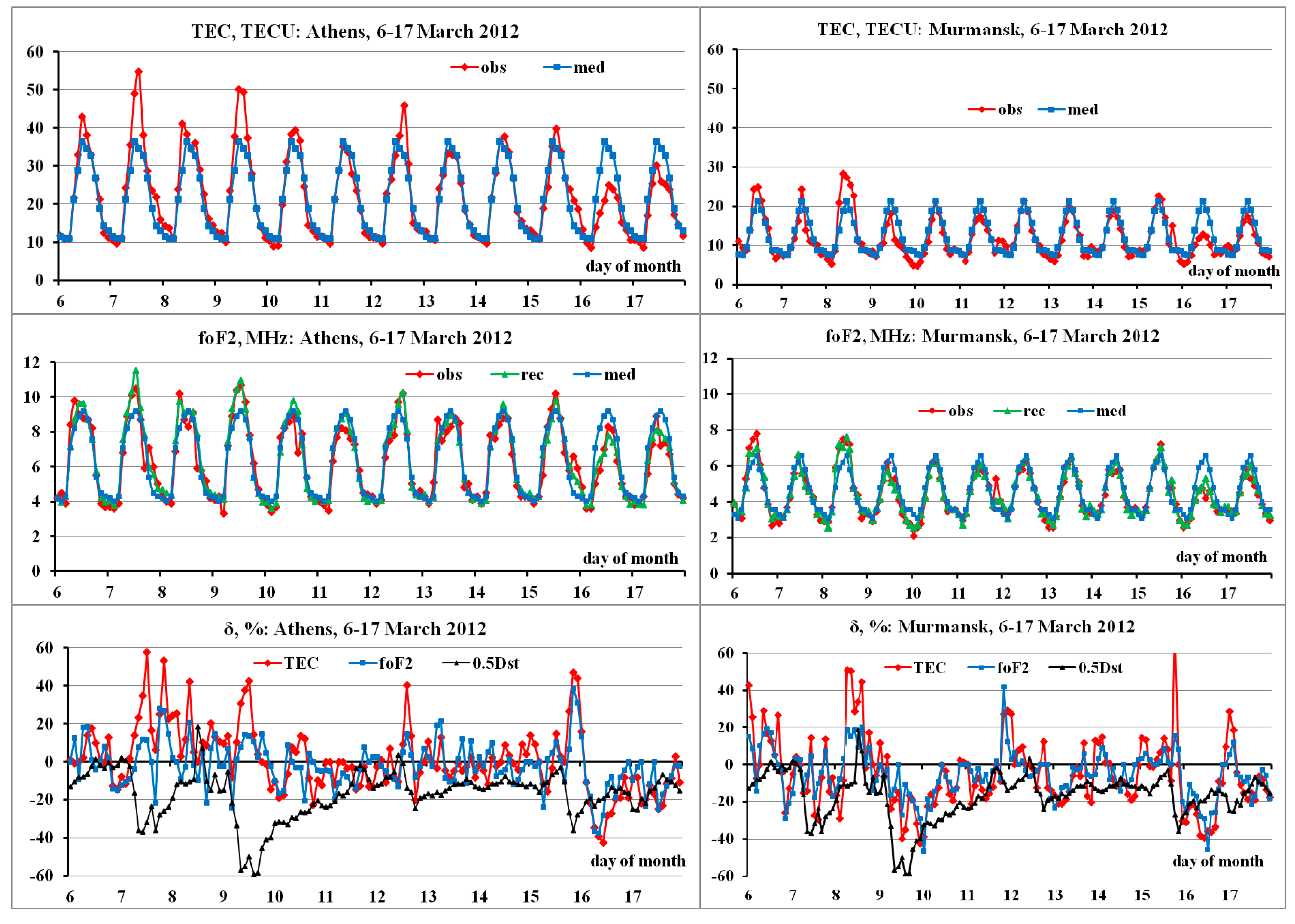
3.1. Behavior of Ionospheric Parameters According to Ionosonde Data

The behavior of TEC; foF2; and their relative deviations, δTEC and δfoF2, from the corresponding medians are shown in Figure 5 for two stations, Athens and Murmansk.
TEC behavior is shown in the upper graphs. The values increase with decreasing latitude. The disturbances are both positive and negative. The average graphs show the behavior of foF2 for three options: observational values (obs icon), medians (med icon) and foF2(rec) values calculated (reconstructed) using observational values of TEC(obs) and median τ(med). It can be seen that the values of foF2(med) are constants, and the values of foF2(rec) are much closer to the observational values than the medians, i.e., they reflect the nature of the disturbance and can be used to reconstruct the disturbance pattern along the meridian. This is confirmed by the behavior of the relative deviations, δTEC and δfoF2, presented in the lower plots along with 0.5Dst values. In this paper, the Dst (disturbance storm time) index, which was developed to study geomagnetic storms, was used to describe a disturbed ionospheric state (e.g., [18,19]). This measures the intensity of a storm and allocates storms into categories: intense (Dst ≤ −100 nT), moderate (−100 nT < Dst < −50 nT), and weak (Dst > −50 nT). We used the Kyoto Dst available at http://wdc.kugi.kyoto-u.ac.jp/dstdir/. One can observe the synchronism of variations of both parameters in response to disturbances.
Figure 5 shows that the ionospheric responses to the storm have both positive and negative phases. In [20], it was specified that magnetic storms can be positive and negative depending on increases or decreases in the electron density, respectively (ТЕС). Six mechanisms were provided for an explanation of positive storms; for negative storms, only changes in neutral composition that led to a decrease in the O/N2 density ratio were considered. In [21], the scheme, including a complicated chain of mechanisms for an explanation of positive disturbances, is presented. It is underlined that there are no insufficient measurements from which to choose a correct explanation for a positive phase.

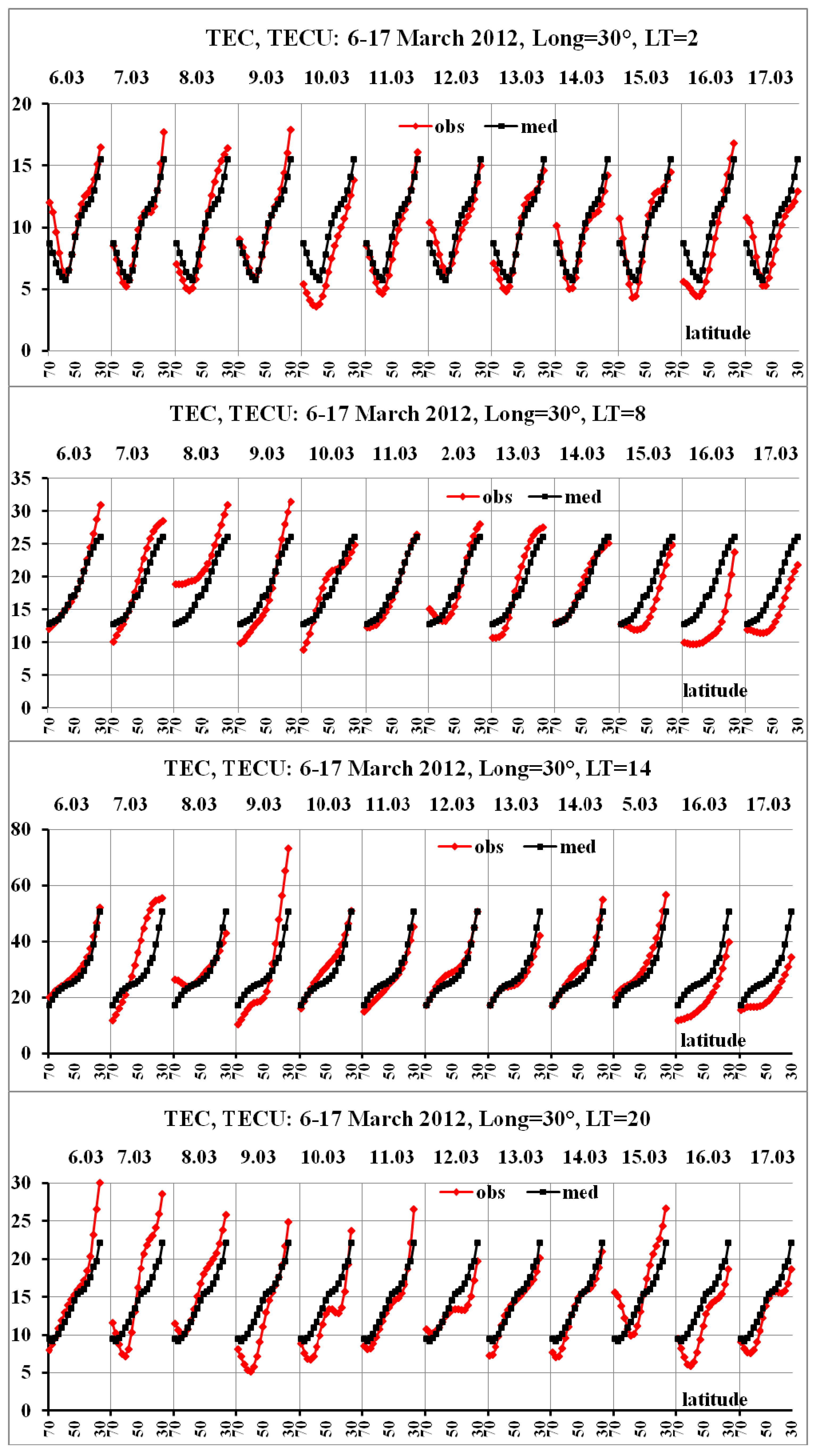
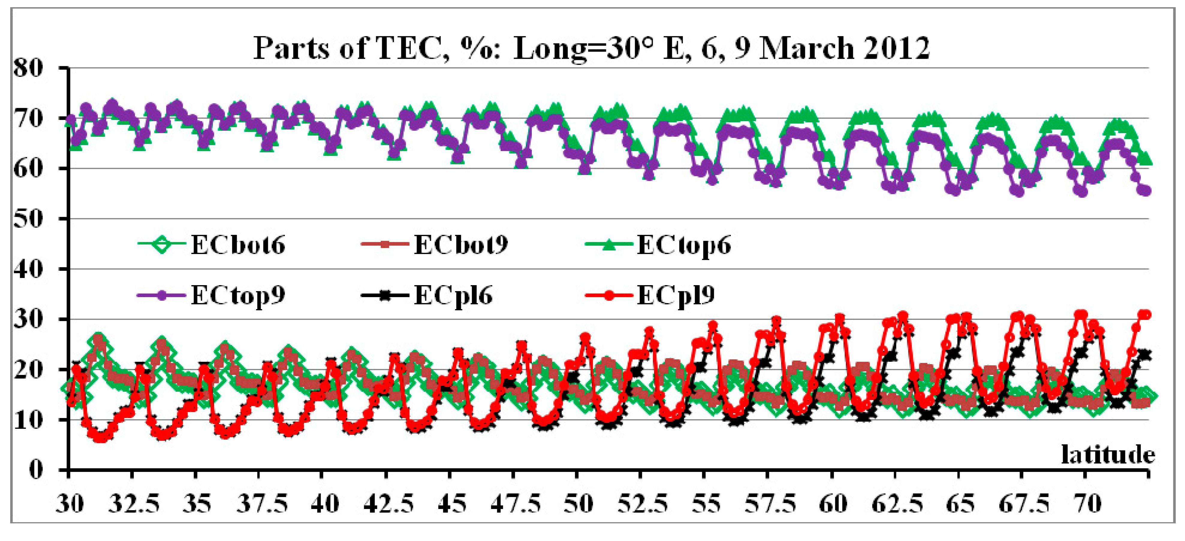
3.2. The Latitudinal Dependence of the TEC Response to Disturbances in the Period 7–17 March 2012

Figure 6 shows examples of the latitudinal dependence of TEC during disturbances along with the behavior of medians for comparison, in the range 30°–70° N, for several hours because some curves coincide. On the Х-axis, latitudes are shown in decreasing order. The longitude is 30° E. Curves are shown for various local times (LT).
Medians are shown in the upper left graph. On 7 March (the upper right panel), a magnetic storm (MS) was caused by the southern component of the interplanetary magnetic field, which led to an increase in ionization and TEC in the daytime. The 9 March magnetic storm had a different nature and a different interplanetary explanation: the speed of the magnetic cloud was high and equal to ~700–740 km/s, which led to an unusually sudden impulse SI+ at ~1130 UT on 8 March [13]. The ionosphere response was also expressed as an increase in TEC, but only at low latitudes (the lower left panel). The picture for 12 March is not shown, because, despite the double shock wave and the beginning of the super-substorm, no significant TEC response was observed. On 15 March, the MS was triggered by the southern component of the IMF, but due to the magnetic cloud and the high-speed solar wind flow, which led to an expansion of the recovery phase, on 16 March, there was a global decrease in TEC (the lower right panel). The full picture is presented in Figure 7 for several hours, at LT = 2, 8, 14 and 20. Each curve for each day represents the latitudinal dependence TEC (latitude), similar to the curves in Figure 6 for separate hours where the latitude changes from 70° N to 30° N in increments of 2.5°, i.e., each curve contains 17 points. Corresponding days are indicated in the top part of the plot, and the days are separated by vertical lines.
The effect of the first MS (increase in TEC) was already visible on the evening of 6 March and the next day; however, there was a change in the signs of disturbance, namely: at high latitudes, a negative disturbance was observed, and at low latitudes, it was positive. The same is true concerning 9 March with maximum TEC. On March 10, at night, there was a negative disturbance at all latitudes. A very minor response on 12 March and an extended recovery phase on 16–17 March after MS on 15 March with global negative disturbance, were confirmed.

3.3. The Latitudinal Dependence of the foF2 Response to Disturbances in the Period 7–17 March 2012

The foF2 values reconstructed through the TEC of the previous section are designated foF2(rec). The latitudinal dependences of the frequencies, foF2(rec), obtained from the observational values of TEC and the median τ(Appr) are shown in Figure 8.
It can be seen that the behavior of the frequencies differs from the medians, reflecting the nature of the disturbances. The nature of the disturbances differs in various zones: positive and negative disturbances, change in the signs of disturbances, testifying the change in mechanisms, are visible.
Correspondence with the previous results lies in the observation of enhancements of daytime TEC in low-latitude zones and an extended recovery phase after the magnetic storm of 15 March on this meridian. Additionally, a deepening of the main trough was obtained at almost all phases of magnetic storms (Figure 8 for LT = 18). The new result consists of a change in the signs of disturbances from high latitudes to low latitudes.

4. Conclusions

This paper specifies models that could be a candidate for the title of a global model of the equivalent ionospheric slab thickness τ. Based on data from four ionosondes located along the 30° E meridian and published sources, four options were compared: τ(IRI), τ(IRI-Plas), τ(NSTM), and τ(Appr). One important problem is the study of the disturbed behavior of the ionosphere along specific meridians; however, there are a small number of meridians along which ionosondes are located. It is shown that in this case it is possible to use a polynomial approximation of τ together with observational values TEC(obs). On meridians along which ionosondes are not present, it is possible to use the IRI-Plas model adapted to TEC(obs). Using the τ(Appr) option, the features of foF2 behavior during the disturbances on 7–17 March 2012, were obtained. Correspondence with the results of other authors at separate points has been shown, and additional new results were obtained, allowing an estimation of the difference in the response of the ionosphere at different latitudinal zones, in particular, the transition from positive to negative disturbances. In this paper, the possibilities of using global models of τ along the meridian are revealed. Even greater possibilities can be provided by using data from satellites, such as DEMETER, Swarm and others, allowing an estimation of the differences in the distribution of parameters in the northern and southern hemispheres at satellite heights, and with the adaptation of the IRI-Plas model to plasma frequencies fne(sat) measured on a satellite, to obtain foF2, if there is TEC, with a high temporal resolution. An additional advantage of the IRI-Plas model is that it allows an estimation of the contribution of different parts of the N(h)-profiles to the TEC value: ECbot—bottomside part (from the beginning of the ionosphere to the height of the maximum hmF2); ECtop—topside part (from the height hmF2 to h ~1300–1500 km); ECpl—plasmaspheric part (from this boundary to the GPS satellite altitude). Figure 9 shows these contributions for 6 March, which is a quiet day, and 9 March with traces of the ionospheric response to the disturbance. Curves for 6 March are very close to a monthly median, i.e., are typical for the whole month. Curves for 9 March show the influence of disturbance. It is necessary to underline that such distribution of contributions is characteristic for all ranges of latitudes.
One can see a significant difference in the structure of the ionosphere depending on latitude. The largest part falls on the topside, but its contribution can decrease during a disturbance. An important result is a large influence of the plasmaspheric part of TEC: the contribution of the plasmaspheric part ECpl can be comparable and even exceed the contribution of ECbot by a factor of 2–3, reaching 30%, which contradicts the tacit assumption about its small size when comparing models that do not take into account the plasmaspheric part with TEC measurements on GPS satellites.
In conclusion, it is necessary to note the emergence of a tendency to diminish the role of the foF2 frequency in the study of the disturbed state of the ionosphere, and switch to using only TEC, since there are many more GPS receivers than ionosondes. The necessity to know foF2 does not decrease because foF2 contributes to the filling of missing periods in long-term statistics. For example, in [22], the authors had to reconstruct the TEC values at the Kokabunji point in the years when there were no TEC measurements. For this, they used two databases, (1) simultaneous measurements of foF2 and TEC over 22 years, and (2) measurements of foF2 over the previous 62 years, when there were no TEC measurements. Based on the data of the first base, a model τ was built, which was used to determine the TEC from the data of the second base. Other examples are shown in the approaches used in [23,24,25].

Author Contributions

Conceptualization, O.M.; methodology, O.M. and A.K.; calculations, O.M., A.K. and T.N.; validation, O.M., A.K. and T.N.; data curation, T.N.; writing—original draft preparation, O.M.; writing—review and editing, O.M. and A.K. All authors have read and agreed to the published version of the manuscript.

Funding

Research was financially supported by the Ministry of Science and Higher Education of the Russian Federation (State assignment in the field of scientific activity, Southern Federal University, No 0852-2020-0015).

Data Availability Statement

GIM TEC values were obtained from IONEX-files, freely available by following the link ftp://cddis.gsfc.nasa.gov/pub/gps/products/ionex. Dst data available on the website http://wdc.kugi.kyoto-u.ac.jp/wdc/Sec3.html.

Acknowledgments

The authors thank the International GNSS Service (IGS) for GPS data and products, groups of scientists providing online IRI-2016 and IRI-Plas models. foF2 data for four stations were taken from the IZMIRAN website https://www.izmiran.ru/ionosphere/weather/foF2/indexss.shtml. Dst data were obtained from http://wdc.kugi.kyoto-u.ac.jp/wdc/Sec3.html. The authors express gratitude to the three reviewers whose comprehensive comments have allowed us to improve the paper significantly.

Conflicts of Interest

The authors declare no conflict of interest.

References

  1. Davies, K. Ionospheric Radio Propagation. National Bureau of Standards Monograph 80; NIST Publications: Gaithersburg, MD, USA, 1 April 1965; 487p. [Google Scholar]
  2. Davies, K.; Liu, X.M. Ionospheric slab thickness in middle and low latitudes. Radio Sci. 1991, 26, 997–1005. [Google Scholar] [CrossRef]
  3. Hernández-Pajares, M.; Juan, J.M.; Sanz, J.; Orus, R.; Garcia-Rigo, A.; Feltens, J.; Komjathy, A.; Schaer, S.C.; Krankowski, A. The IGS VTEC maps: A reliable source of ionospheric information since 1998. J. Geod. 2009, 83, 263–275. [Google Scholar] [CrossRef]
  4. Bilitza, D.; Altadill, D.; Truhlik, V.; Shubin, V.; Galkin, I.; Reinisch, B.; Huang, X. International Reference Ionosphere 2016: From ionospheric climate to real-time weather predictions. Space Weather 2017, 15, 418–429. [Google Scholar] [CrossRef]
  5. Gulyaeva, T. International standard model of the Earth’s ionosphere and plasmasphere. Astron. Astrophys. Trans. 2003, 22, 639–643. [Google Scholar] [CrossRef]
  6. Hoque, M.M.; Jakowski, N. A new global empirical NmF2 model for operational use in radio systems. Radio Sci. 2011, 46, RS6015. [Google Scholar] [CrossRef]
  7. Jakowski, N.; Hoque, M.M.; Mayer, C. A new global TEC model for estimating transionospheric radio wave propagation errors. J. Geod. 2011, 85, 965–974. [Google Scholar] [CrossRef]
  8. Jakowski, N.; Hoque, M.; Mielich, J.; Hall, C. Equivalent slab thickness of the ionosphere over Europe as an indicator of long-term temperature changes in the thermosphere. J. Atmos. Sol. Terr. Phys. 2017, 163, 91–102. [Google Scholar] [CrossRef]
  9. Fron, A.; Galkin, I.; Krankowski, A.; Bilitza, D.; Hernández-Pajares, M.; Reinisch, B.; Li, Z.; Kotulak, K.; Zakharenkova, I.; Cherniak, I.; et al. Towards Cooperative Global Mapping of the Ionosphere: Fusion Feasibility for IGS and IRI with Global Climate VTEC Maps. Remote Sens. 2020, 12, 3531. [Google Scholar] [CrossRef]
  10. Jakowski, N.; Hoque, M.M. Global equivalent slab thickness model of the Earth’s ionosphere. J. Space Weather Space Clim. 2021, 11, 1–18. [Google Scholar] [CrossRef]
  11. Galkin, I.A.; Reinisch, B.W.; Bilitza, D. Realistic Ionosphere: Real-time ionosonde service for ISWI. SunGe 2018, 13, 173–178. [Google Scholar]
  12. Gulyaeva, T.L.; Arikan, F.; Hernandez-Pajares, M.; Stanislawska, I. GIM-TEC adaptive ionospheric weather assessment and forecast system. J. Atmos. Sol. Terr. Phys. 2013, 102, 329–340. [Google Scholar] [CrossRef] [Green Version]
  13. Tsurutani, B.; Echer, E.; Shibata, K.; Verkhoglyadova, O.; Mannucci, A.; Gonzalez, W.D.; Kozyra, J.U.; Pätzold, M. The interplanetary causes of geomagnetic activity during the 7–17 March 2012 interval: A CAWSES II overview. J. Space Weather Space Clim. 2014, 4, A02. [Google Scholar] [CrossRef] [Green Version]
  14. Belehaki, A.; Kutiev, I.; Marinov, P.; Tsagouri, I.; Koutroumbas, K.; Elias, P. Ionospheric electron density perturbations during the 7–10 March 2012 geomagnetic storm period. Adv. Space Res. 2017, 59, 1041–1056. [Google Scholar] [CrossRef]
  15. Verkhoglyadova, O.P.; Tsurutani, B.T.; Mannucci, A.J.; Mlynczak, M.G.; Hunt, L.A.; Paxton, L.J. Ionospheric TEC, thermospheric cooling and Σ[O/N2] compositional changes during the 6–17 March 2012 magnetic storm interval (CAWSES II). J. Atmos. Sol. Terr. Phys. 2014, 115–116, 41–51. [Google Scholar] [CrossRef]
  16. Gulyaeva, T.L. Modification of solar activity indices in the international reference ionosphere IRI and IRI-Plas models due to recent revision of sunspot number time series. Sol. Terr. Phys. 2016, 2, 87–98. [Google Scholar] [CrossRef]
  17. Huang, H.; Liu, L.; Chen, Y.; Le, H.; Wan, W. A global picture of ionospheric slab thickness derived from GIM TEC and COSMIC radio occultation observations. J. Geophys. Res. Space Phys. 2016, 121, 867–880. [Google Scholar] [CrossRef]
  18. Anh, V.V.; Yu, Z.; Wanliss, J.A.; Watson, S.M. Prediction of magnetic storm events using the Dst index. Nonlinear Process. Geophys. 2005, 12, 799–806. [Google Scholar] [CrossRef] [Green Version]
  19. Balan, N.; Tulasiram, S.; Kamide, Y.; Batista, I.S.; Souza, J.R.; Shiokawa, K.; Rajesh, P.K.; Victor, N.J. Automatic selection of Dst storms and their seasonal variations in two versions of Dst in 50 years. Earth Planets Space 2017, 69, 59. [Google Scholar] [CrossRef] [Green Version]
  20. Fagundes, P.R.; Cardoso, F.A.; Fejer, B.G.; Venkatesh, K.; Ribeiro, B.A.G.; Pillat, V.G. Positive and negative GPS-TEC ionospheric storm effects during the extreme space weather event of March 2015 over the Brazilian sector. J. Geophys. Res Space Phys. 2016, 121, 5613–5625. [Google Scholar] [CrossRef] [Green Version]
  21. Prölss, G.W. Ionospheric F-region Storms: Unsolved Problems. In Characterising the Ionosphere (10-1–10-20). Meeting Proceedings RTO-MP-IST-056; RTO: Neuilly-sur-Seine, France, 2006; p. 10. Available online: http://www.rto.nato.int/abstracts.asp (accessed on 7 September 2021).
  22. Nishioka, M.; Saito, S.; Tao, C.; Shiota, D.; Tsugawa, T.; Ishii, M. Statistical analysis of ionospheric total electron content (TEC): Long-term estimation of extreme TEC in Japan. Earth Planets Space 2021, 73, 52. [Google Scholar] [CrossRef]
  23. Gerzen, T.; Jakowski, N.; Wilken, V.; Hoque, M.M. Reconstruction of F2 layer peak electron density based on operational vertical total electron content maps. Ann. Geophys. 2013, 31, 1241–1249. [Google Scholar] [CrossRef] [Green Version]
  24. Krankowski, A.; Shagimuratov, I.I.; Baran, L.W. Mapping of foF2 over Europe based on GPS-derived TEC data. Adv. Space Res. 2007, 39, 651–660. [Google Scholar] [CrossRef]
  25. Pignalberi, A.; Habarulema, J.B.; Pezzopane, M.; Rizzi, R. On the development of a method for updating an empirical climatological ionospheric model by means of assimilated vTEC measurements from a GNSS receiver network. Space Weather 2019, 17, 1131–1164. [Google Scholar] [CrossRef] [Green Version]
Figure 1. The diurnal variation of the initial medians of the equivalent slab thickness (the left panel) and an example of dependencies calculated for three latitudes in accordance with the polynomial approximation (the right panel).
Universe 07 00342 g001
Figure 2. Latitudinal dependence of the median of the equivalent slab thickness, calculated according to the data of four ionosondes lying near the longitude of 30° E.
Universe 07 00342 g002
Figure 3. Comparison of τ for different models.
Universe 07 00342 g003
Figure 4. Diurnal variation of the observed and modeled τ over Tromsø for January 2000–2008.
Universe 07 00342 g004
Figure 5. Statistics of the disturbed state according to the data of two stations, including changes in the parameters TEC and foF2 and their relative deviations, δTEC and δfoF2.
Universe 07 00342 g005
Figure 6. Examples of the ionosphere response to disturbances along the 30° E meridian.
Universe 07 00342 g006
Figure 7. The response of the TEC parameter to the disturbances of 7–17 March 2012, at various hours of the day.
Universe 07 00342 g007
Figure 8. Response of frequency foF2(rec) to disturbances on 7–17 March 2012, at various hours of the day.
Universe 07 00342 g008
Figure 9. Contributions of bottomside, topside and plasmaspheric parts to the total TEC value.
Universe 07 00342 g009
Table 1. τ metrics for four stations.
0246810121416182022
AthRSME81.464.0105.385.862.753.049.459.790.3111.6140.067.8
NRSME15.511.622.125.218.114.315.017.124.021.524.612.0
MosRSME273.5257.193.590.198.268.747.253.3144.5171.6186.8292.8
NRSME37.530.227.027.831.719.514.015.136.737.127.135.8
MurRSME136.191.7106.050.450.563.056.544.8175.5152.2125.9115.2
NRSME23.914.618.110.411.514.116.111.944.434.323.021.8
LonRSME223156137207205249159129225198133215
NRSME352722444753352851432838
Publisher’s Note: MDPI stays neutral with regard to jurisdictional claims in published maps and institutional affiliations.

