Constraining the Swiss-Cheese IR-Fixed Point Cosmology with Cosmic Expansion

Abstract

A recent work proposed that the recent cosmic passage to a cosmic acceleration era is the result of the existence of small anti-gravity sources in each galaxy and clusters of galaxies. In particular, a Swiss-cheese cosmology model, which relativistically integrates the contribution of all these anti-gravity sources on a galactic scale has been constructed assuming the presence of an infrared fixed point for a scale dependent cosmological constant. The derived cosmological expansion provides an explanation for both the fine tuning and the coincidence problem. The present work relaxes the previous assumption on the running of the cosmological constant and allows for a generic scaling around the infrared fixed point. Our analysis reveals that, in order to produce a cosmic evolution consistent with the best $\Lambda$CDM model, the IR-running of the cosmological constant is consistent with the presence of an IR-fixed point.

1. Introduction

The cosmological constant problem of quantum field theory, first emphasized by Zeldovich, is one of the greatest problems of modern theoretical physics. Even if one would expect quantum gravity to offer an explanation as to why the vacuum does not gravitate (due to non perturbative effects), the natural thing is to have, for the present cosmic time, a zero (negligible) cosmological constant; otherwise, a fine tuning problem emerges as in the $\Lambda$CDM phenomenological model.

However, the recent cosmic acceleration [1,2,3,4] adds more mystery to the problem. This missing amount of dark energy (DE) [5], is possibly the result of a time varying cosmological constant $\Lambda \left(z\right)$. There are many papers that have attempted to explain this recent low redshift cosmic acceleration. Among them, there are two proposed solutions without the fine tuning problem, [6,7]. They remove the coincidence and fine tuning problem connecting the recent large scale structure and its characteristics with the recent cosmic acceleration.

The present study concerns a further elaboration of the second work [7], connecting it and testing it with the cosmological observational data. There are also some other works [8,9,10,11,12,13] that attempted to resolve (partially or fully) the recent cosmic acceleration and coincidence problem using the recent large scale structure formation; however, these works associate inhomogeneities with the change of the expansion rate. In [7], local antigravity sources are the reason for the solution, and no inhomogeneities play any role. We expect that the inclusion of inhomogeneities will further help with generation of the cosmic acceleration.

In [7], the proposed solution was based on the infrared quantum gravity modifications at the astrophysical scales. These corrections result in a non-zero positive cosmological constant that is related to astrophysical configurations of matter and energy, such as galaxies or clusters of galaxies. Thus, antigravity sources are effectively generated. Such quantum gravity corrections are, perhaps, possible in the framework of the Asymptotic Safety (AS) program for quantum gravity [14,15,16].

Summing, relativistically, all homogeneously distributed anti-gravity sources from every galaxy or cluster of galaxies, we obtain a net effect on the cosmic expansion. This “sum” can be performed adapting a Swiss-cheese model in which matching between the local and the cosmic patches generates the observed recent passage from deceleration to acceleration.

In the last ten years, many cosmological models have been developed to explain DE. Some of them are of a more geometric origin using geometric modifications of general relativity, while some of them consider quantum effects and/or particle physics phenomena and exotic fields. Several are mainly phenomenological solutions, while others are more close to theoretical concrete models. Therefore, it is vital to evaluate all of them using observational data [17,18].

The relevant criteria are how well they agree with the characteristics of the late expansion of the universe. The features of the cosmic history can be revealed using supernovae, SNIa [19], Gamma Ray Bursts (GRB) [20,21,22,23], or HII galaxies [24,25], as luminosity distance estimators. An alternative method of testing is in using the angular diameter distance coming from clusters or CMB sound horizon via Baryon Acoustic Oscillations (BAO) [26,27], or in utilizing the CMB angular power spectrum [28]. Other probes of the characteristics of the cosmic expansion are measures of the growth rate of matter perturbations. Galaxies are also very good cosmic chronometers [17], and the observations of their growth rates [29] provide knowledge that is independent of the implied cosmological model for the the integral of the Hubble parameter $H\left(z\right)$.

In [30,31], the cosmological model proposed in [7] was tested against observational data sets: (1) measurements of the Hubble rate $H\left(z\right)$, (2) Supernovae Ia (Pantheon data set, (3) Quasi-Stellar-Objects (QSO), (4) Baryonic Acoustic Oscillations, and (5) direct measurements of the CMB shift parameters. The result was that the model was in very good agreement with the observations.

In the present work, we instead test the possibility of a more general scaling law for the cosmological constant consistent with the presence of a deviation from the canonical scaling, which we parametrize by means of an anomalous dimension $\eta$. In particular, we tested the consistency of our model against the backdrop of LCDM cosmology with fiducial values taken from the current observational best fits solutions.

There are two novelties in the present work. In [7], the authors used a phenomenological term for $\Lambda$, while, here, we point out for the first time that this term can be interpreted as an anomalous dimension due to quantum non-perturbative corrections. Furthermore, in the present work, we analyze how sensitive the correct phenomenology of the late cosmology is to the value of b. In [7], the authors claimed that there is no fine tuning in dimensionless parameters. This, indeed, is true. The present paper proves thoroughly that we do not have such fine tuning. We do not need a very precise value of b to obtain correct behavior.

The structure of the article is as follows: in Section 2, we present the theoretical aspects of the Asymptotically Safe Swiss-cheese gravity. In Section 3, we discuss the observational data sets that we employ along with our method and the corresponding results. Finally, we summarize our conclusions in Section 4.

2. Swiss-Cheese Model and IR-Fixed Point Cosmology

2.1. Asymptotic Safety in UV and IR

In the Asymptotic Safety scenario, the UV behavior of gravity is ruled by a non-perturbative fixed point of the renormalization group for quantum gravity [32,33]. The essential ingredient of this approach is the Effective Average Action, a Wilsonian coarse-grained free energy dependent on an infrared momentum scale k, which defines an effective field theory appropriate for the scale k. By construction, when evaluated at the tree level, the Effective Average Action correctly describes all gravitational phenomena, including all loop effects, if the typical momentum involved are of the order of k. When applied to the Einstein–Hilbert action, the ERG yields renormalization group flow equations, which have made possible detailed investigations of the scaling behavior of Newtons constant at high energies.

The scenario emerging from these studies (see [34] for a recent discussion on the AS scenario and its potential application) suggests that the theory could be consistently defined in $d=4$ at a nontrivial UV fixed point where the dimensionless Newton constant, $g\left(k\right)=G\left(k\right)k^2$ does not vanish in the $k\to \infty$ limit. As a consequence, the dimensionful Newton constant $G\left(k\right)$ is antiscreened at high energies, as one would expect based on the intuitive picture that the larger is the cloud of virtual particles, and the greater is the effective mass seen by a distant observer [35].

Albeit, in the original formulation of the AS approach, the UV non-Gaussian fixed point emerging in the UV at transplanckian energies to recover the continuum limit, it has been realized that a non-perturbative IR fixed point at small k could solve the singular behavior of the $\beta$-functions assuming that a sort of tree level renormalization could take place at large distances, so that

$$\begin{array}{c}\hfill G\left(k\right)=g_{\ast }/k^2\Lambda \left(k\right)={\lambda }_{\ast }{k}^2\end{array}$$

(1)

for $k\to 0$. Clearly, k should be considered not as a momentum flowing into a loop, but as an inverse of a typical distance over which the averaging of the field variables is performed. From this point of view, several works have discussed the possibility of interpreting astrophysical data as an infrared effect of quantum gravity, relating k to a cosmic time [36], or cosmic distance. In particular, in [7], the running scale k is connected with the typical size of a galaxy or of a cluster of galaxies embedded in a Swiss-cheese cosmological model. For this reason, this approach is closer in spirit to the scale identification proposed in [37,38,39].

In this work, we assume that there is no significant running of G at cosmological scale [40]; however, we allow for the possibility of deviation from the canonical scaling in the running of $\Lambda$. In particular, we set $g_{\ast }/k^2\sim constant$ and $\Lambda \left(k\right)={\lambda }_{\ast }{k}^{2-\eta }$ where $\eta$ is the anomalous dimension [41]. As explained in [41], the varying behavior of the cosmological constant is based on the instability induced renormalization triggered by the low energy quantum fluctuations in a Universe with a positive cosmological constant. For $\eta =0$, the canonical (mean-field) scaling is recovered.

In the following, we write $b\equiv 2-\eta$, and b has to be determined by assuming an underling best-fit $\Lambda$CDM cosmology.

2.2. AS Swiss-Cheese

This section provides a summary of the mathematical description of the AS inspired Swiss-cheese cosmological model presented in [7]. The Swiss-cheese model or otherwise called Einstein–Strauss model [42] describes a global homogeneous and isotropic metric, the Universe, with many local Schwarzschild black hole metrics homogeneously distributed. The geometrical covariant matching of the global metric as the exterior solution with a local interior spherical solution happens across a spherical boundary that is proven to be at a constant coordinate radius of the cosmological metric but at a spherical solution’s radius evolving in time.

In more detail, we geometrically match the exterior background spacetime described by a Friedmann-Lemaître-Robertson-Walker (FLRW) metric to an interior local black hole metric. This happens on a spherical 3-surface, $\Sigma$, of constant coordinate radius in the FLRW frame but time evolving in the Schwarzschild frame. The matching of the two solutions makes use of the first fundamental form (intrinsic metric) and the second fundamental form (extrinsic curvature), calculated in terms of the coordinates on $\Sigma$, on both sides [43].

In our case, we use, as a local solution, the AS-inspired corrected Schwarzschild–de Sitter metric. This quantum improved Schwarzschild-de Sitter metric contains energy dependent cosmological and Newton constants with the hope to describe fairly astrophysical objects, such as clusters of galaxies. Thus, in the metric, there are energy dependent $G_k=G\left(k\right)\sim G_N,{\Lambda }_k=\Lambda \left(k\right)={\lambda }_{\ast }^{IR}{k}^b$. So

$$d{s}^2=-\left(1-\frac{2G_{k}M}{R}-\frac{1}{3}{\Lambda }_k{R}^2\right)d{T}^2+\frac{d{R}^2}{1-\frac{2G_{k}M}{R}-\frac{1}{3}{\Lambda }_k{R}^2}+R^{2}d{\Omega }^2,$$

(2)

where, now, both Newton’s constant $G_k$ and the cosmological constant ${\Lambda }_k$ are functions of a characteristic scale k of the system determined by the quantum gravity theory in use.

The previous metric should be matched with a homogeneous and isotropic metric. The cosmological metric is of the form

$$d{s}^2=-d{t}^2+a^2\left(t\right)\left[\frac{d{r}^2}{1-\kappa r^2}+r^{2}d{\Omega }^2\right],$$

(3)

where $a\left(t\right)$ is the scale factor and $\kappa =0,\pm 1$ characterizes the spatial curvature and $d{\Omega }^2=\left(d{\theta }^2+{sin}^2\theta d{\phi }^2\right)$ characterizes the metric of the two spheres.

We work on a 4-dimensional spacetime M and with a metric $g_{\mu \nu }$. There is a time-like hypersurface $\Sigma$ that divides M into two regions. The hypersurface $\Sigma$ has induced metric $h_{\mu \nu }=g_{\mu \nu }-n_{\mu }{n}_{\nu }$, with $n^{\mu }$ the unit normal vector to $\Sigma$ pointing inwards. The extrinsic curvature is given by $K_{\mu \nu }=h_{\mu }^{\kappa }{h}_{\nu }^{\lambda }{n}_{\kappa ;\lambda }$. Covariant differentiation with respect to $g_{\mu \nu }$ is denoted by the semicolon “;”. The formalism permits the use of different coordinate systems on both sides of the hypersurface in Darmois–Israel junction conditions [44,45].

Darmois–Israel junction conditions are the two conditions for smooth matching. The matching conditions require the continuity of spacetime across $\Sigma$. The latter means a continuity of the induced metric $h_{ij}$ on $\Sigma$. The Darmois–Israel matching conditions also demand the sum of the two extrinsic curvatures computed on the two sides of $\Sigma$ to be zero.

The first fundamental form is the induced metric on $\Sigma$ and is equal to

$${\gamma }_{\alpha \beta }=g_{ij}\frac{\partial x^i}{\partial u^{\alpha }}\frac{\partial x^j}{\partial u^{\beta }},$$

(4)

with $u^{\alpha }=(u^1\equiv u,u^2\equiv v,u^3\equiv w)$ as the coordinate system on $\Sigma$ while $\alpha ,\beta$ take integer values $1,\dots ,3,$ and english indices $i,j$ run over $1,\dots ,4.$

The second fundamental form is given by

$$K_{\alpha \beta }=n_{i;j}\frac{{\gamma }_{\alpha \beta }}{g_{ij}}=({\Gamma }^p{}_{ij}{n}_p-n_{i,j})\frac{\partial x^i}{\partial u^{\alpha }}\frac{\partial x^j}{\partial u^{\beta }},$$

(5)

where ${\Gamma }^p{}_{ij}$ are the Christoffel symbols.

Note that the cosmic evolution through the Swiss-cheese is determined by the cosmic evolution of the matching surface that is happening at the sphericial radius, in the black hole frame, $R_S$ (and constant $r_{\Sigma }$ for the FLRW frame). This quantity enters the differential equations. The subscript S is after Schucking, and the radius is called the Schucking $R_S$ radius.

The matching requirements provide the following equations for $R_S$,

$$\begin{array}{ccc}\hfill R_S& =& a{r}_{\Sigma }\hfill \end{array}$$

(6)

$$\begin{array}{ccc}\hfill {\hspace{1em}\hspace{1em}\hspace{1em}\hspace{1em}\hspace{1em}\hspace{1em}\hspace{1em}\hspace{1em}\hspace{1em}\left(\frac{d{R}_S}{dt}\right)}^2& =& 1-\kappa r_{\Sigma }^2-\left(1-\frac{2G_{k}M}{R_S}-\frac{1}{3}{\Lambda }_k{R}_S^2\right)\hfill \end{array}$$

(7)

$$\begin{array}{ccc}\hfill \hspace{1em}\hspace{1em}\hspace{1em}\hspace{1em}\hspace{1em} \hspace{1em}\hspace{1em}2\frac{d^2{R}_S}{d{t}^2}& =& -\frac{d\left(1-\frac{2G_{k}M}{R}-\frac{1}{3}{\Lambda }_k{R}^2\right)}{dR}{|}_{R_S}\hfill \end{array}$$

(8)

The matching radius $r_{\Sigma }$ can be understood as the boundary of the volume of the interior solid with energy density equal to the cosmic matter density $\rho$. Thus, the interior energy content should equal the mass M of the astrophysical object, i.e.,

$$r_{\Sigma }=\frac{1}{a_0}{\left(\frac{2G_{N}M}{{\Omega }_{m0}{H}_0^2}\right)}^{\frac{1}{3}},$$

(9)

where the density parameter is ${\Omega }_m=\frac{8\pi G_N\rho }{3H^2}=\frac{2G_{N}M}{r_{\Sigma }^3{a}^3{H}^2}$ and $a_0$, in the following of the study, is set to 1.

Equations (6)–(8) for constant $G_k$ and ${\Lambda }_k$ reduce to the conventional FLRW expansion equations. However, although these equations generate the standard cosmological equations of the $\Lambda \mathrm{CDM}$ model, even in this case the interpretation is different since the $\Lambda$ term appearing in the black hole metric (2) is like an average of all anti-gravity sources inside the Schucking radius of a galaxy or cluster of galaxies. These antigravity sources may arise inside astrophysical black holes in the centers of which the presence of a quantum repulsive pressure could balance the attraction of gravity to avoid the not desired singularity, or it may arise due to IR quantum corrections of a concrete quantum gravity theory. Furthermore, for constant $G_k$ and ${\Lambda }_k$, the coincidence problem is removed since the large scale structure appeared recently.

2.3. Cosmic Acceleration and Coincidence Problem

The meaning of the quantity k is understood in a statistical-mechanical sense. The role of the cutoff k is associated with the block-spin transformation, or Kadanoff blocking, a technique used in lattice field theory and condensed matter [46]. The quantity k is not related to a momentum exchanged in a scattering process of the RG scale often used in dimensional regularization in effective field theory [47]. Assuming Fourier transformability of the block-spin transformation, k is of the order of the inverse of the lattice size. Several scaling behaviors for k have been proposed in astrophysical [48,49] and cosmological contexts [50,51,52,53].

We use the approach in [7] where k has to be associated with a characteristic astrophysical length scale L. Thus, $k=\xi /L$, with $\xi$ is a dimensionless order-one number. A first choice could be L to be the radial distance R from the center. However, this choice proved to be not successful. In [7], we demonstrated that, for $k=\xi /R$, the behavior of the coefficient of equation of dark energy state $w_{DE}$ is wrong.

There is, perhaps, a chance to obtain an acceptable behavior if one includes the redshift dependence of the cluster mass; however, this remains to be shown. Another more physically natural option and, at the same time, generating the correct phenomenology, is to set, as L, the proper distance $D>0$. With this choice, studies also showed a singularity avoidance/smoothing [54,55,56].

The proper distance of a radial curve with $dT=d\theta =d\phi =0$ from $R_0$ until R is estimated by the formula

$$D\left(R\right)={\int }_{R_0}^R\frac{d\mathcal{R}}{\sqrt{1-\frac{2G_{k}M}{\mathcal{R}}-\frac{1}{3}{\Lambda }_k{\left(\mathcal{R}\right)}^2}}.$$

(10)

As we already mentioned, the matching happens at the Schucking radius. This means that the relevant value of k is $k_S=\xi /D_S$, where $D_S\left(R_S\right)$ is the proper distance of the Schucking radius.

Using Equations (6)–(8), it was shown that [7] the Hubble evolution is given by the system

$$\begin{array}{ccc}\hfill H^2& =& -\frac{\kappa }{a^2}+\frac{2G_{N}M}{r_{\Sigma }^3{a}^3}+\frac{\gamma {\xi }^b}{3D_S^b}\hfill \end{array}$$

(11)

$$\begin{array}{ccc}\hfill {\dot{D}}_S& =& r_{\Sigma }aH{\left(1-\frac{2G_{N}M}{r_{\Sigma }a}-\frac{\gamma {\xi }^b{r}_{\Sigma }^2{a}^2}{3D_S^b}\right)}^{-1/2}\hfill \end{array}$$

(12)

where $\gamma ={\lambda }_{\ast }^{IR}$ and the variable $D_S$ is of geometrical nature with its own equation of “motion” (time evolution).

One can further prove that the expansion rate of the scale factor is given by

$$\frac{H^2\left(z\right)}{H_0^2}={\Omega }_{m0}{(1+z)}^3+{\left[{\Omega }_{DE,0}^{-\frac{1}{b}}-\frac{3^{\frac{1}{b}}}{\xi {\tilde{\gamma }}^{\frac{1}{b}}}{\left(G_N{H}_0^2\right)}^{\frac{1}{b}}\frac{r_{\Sigma }{a}_0}{\sqrt{G_N}}\frac{z}{1+z}\right]}^{-b}+{\Omega }_{\kappa 0}{(1+z)}^2,$$

(13)

where we have reparameterized $\gamma$ to the dimensionless $\tilde{\gamma }=\gamma G_N^{1-b/2}$. The acceleration is very well approximated, as before, as a function of z by the expression

$$\frac{\ddot{a}}{H_0^{2}a}=-\frac{1}{2}{\Omega }_{m0}{(1+z)}^3+\left[{\Omega }_{DE,0}^{-\frac{1}{b}}-\frac{3^{\frac{1}{b}}}{2\xi {\tilde{\gamma }}^{\frac{1}{b}}}{\left(G_N{H}_0^2\right)}^{\frac{1}{b}}\frac{r_{\Sigma }{a}_0}{\sqrt{G_N}}\frac{b+2z}{1+z}\right]{\left[{\Omega }_{DE,0}^{-\frac{1}{b}}-\frac{3^{\frac{1}{b}}}{\xi {\tilde{\gamma }}^{\frac{1}{b}}}{\left(G_N{H}_0^2\right)}^{\frac{1}{b}}\frac{r_{\Sigma }{a}_0}{\sqrt{G_N}}\frac{z}{1+z}\right]}^{-1-b}.$$

(14)

and the equation of the state parameter is

$$w_{DE}=\left[\frac{3^{\frac{1}{b}-1}}{\xi {\tilde{\gamma }}^{\frac{1}{b}}}{\left(G_N{H}_0^2\right)}^{\frac{1}{b}}\frac{r_{\Sigma }{a}_0}{\sqrt{G_N}}\frac{b+3z}{1+z}-{\Omega }_{DE,0}^{-\frac{1}{b}}\right]{\left[{\Omega }_{DE,0}^{-\frac{1}{b}}-\frac{3^{\frac{1}{b}}}{\xi {\tilde{\gamma }}^{\frac{1}{b}}}{\left(G_N{H}_0^2\right)}^{\frac{1}{b}}\frac{r_{\Sigma }{a}_0}{\sqrt{G_N}}\frac{z}{1+z}\right]}^{-1}$$

(15)

In the present study, we test Equations (13) and (15) against observations. The free parameters are b, $\xi ,$ and $\tilde{\gamma }$. The values of $\xi$, and $\tilde{\gamma }$ are not known but are expected to be of order O(1). The crucial one is b since it is related to the anomalous dimension that arises due to non-perturbative quantum corrections, and thus the analysis will focus on this. The model does not have many free parameters, and it is remarkable that it provides the correct phenomenology.

We chose the values of the free parameters as follows: One can choose any value of order one for $\xi$ and $\tilde{\gamma }$, and then b must have a value that ensures that the second term and the third term of Equation (11) are almost equal. There must be a balance between attraction and repulsion for low redshifts. Selecting other values for $\xi$ and $\tilde{\gamma }$ changes slightly the value of b for the correct phenomenology. Not only the proper distance today $D_{S,0}$ but also the whole function $D_S\left(z\right)$ remains for all observational tests for the range of redshift z of the order of $r_{\Sigma }$.

3. Methodology and Numerical Results

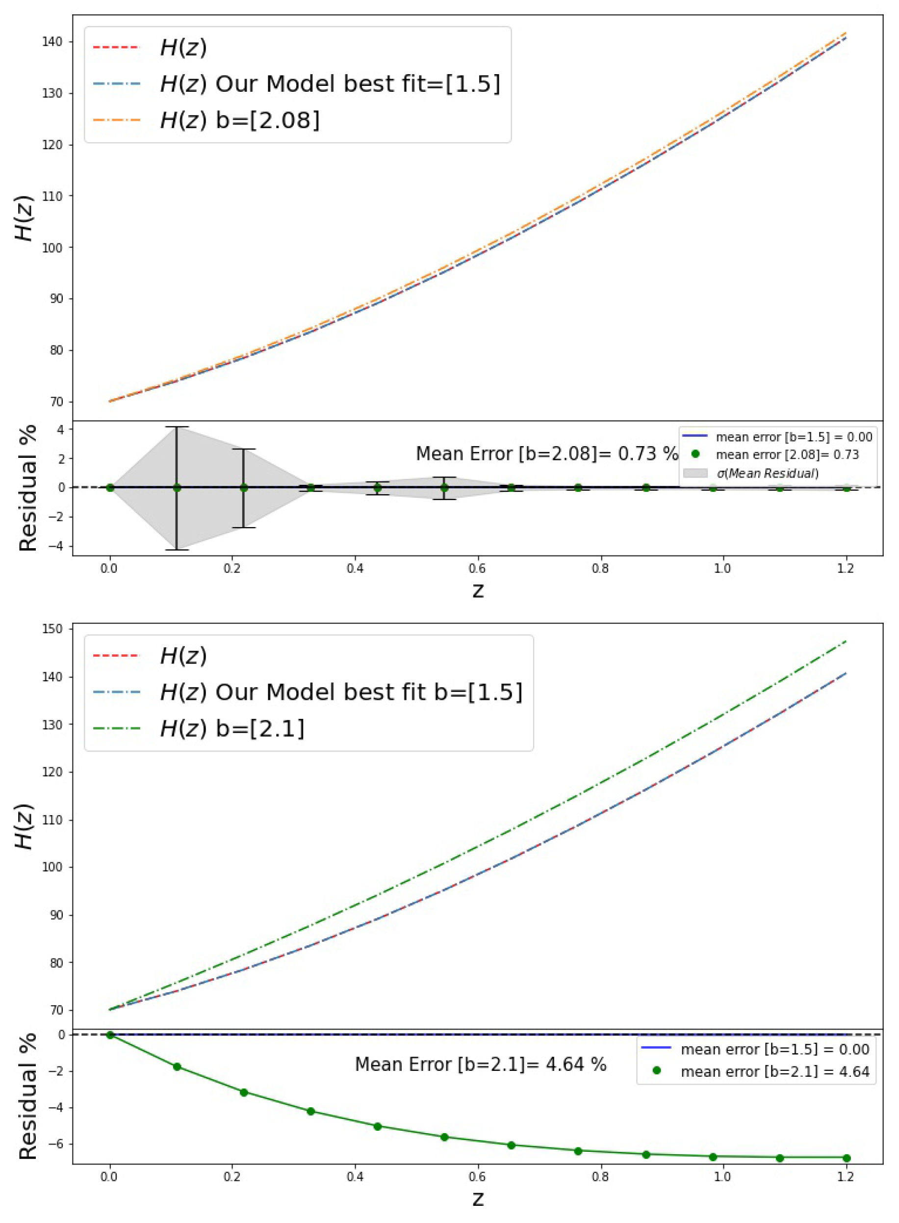
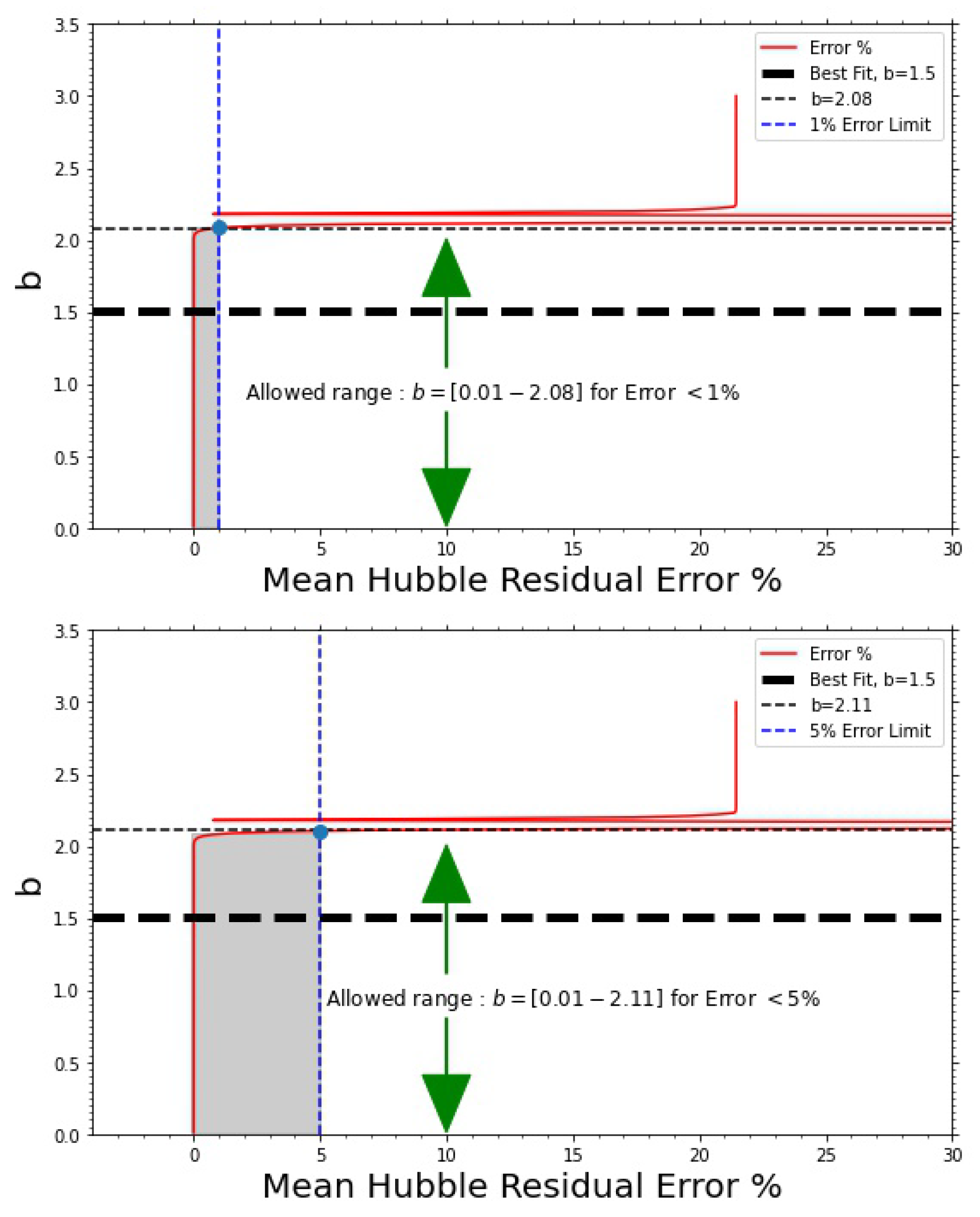
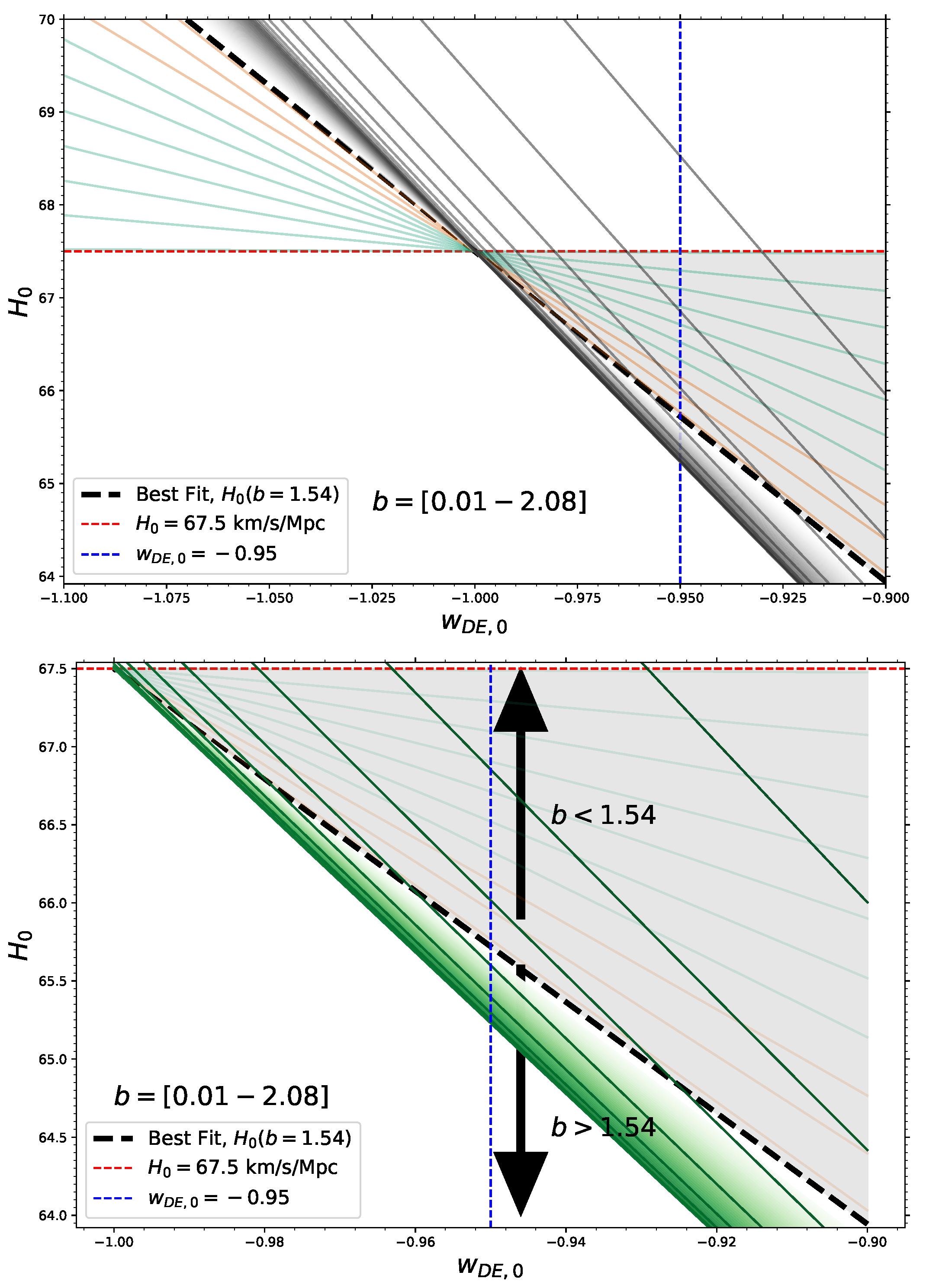
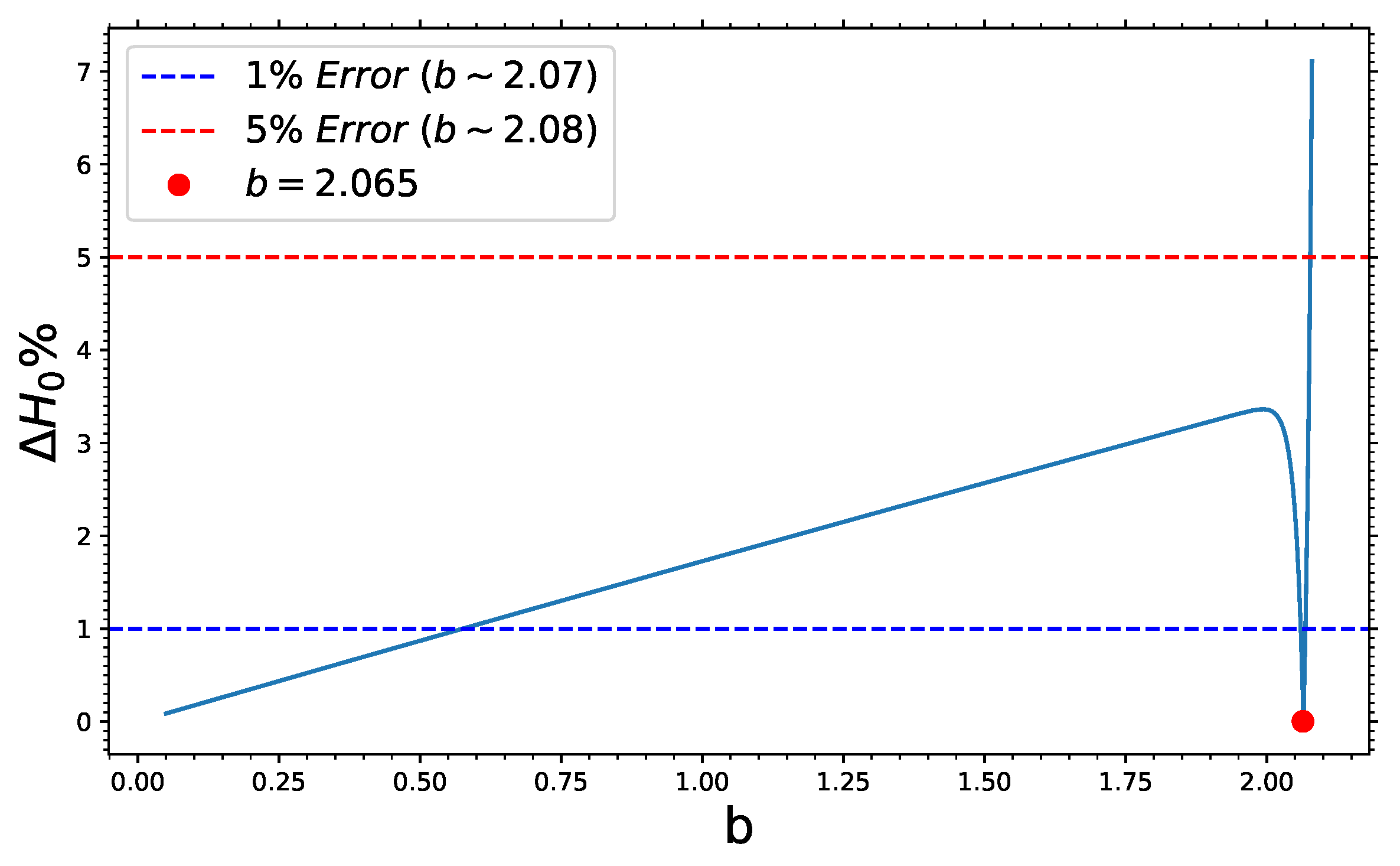
For the comparison of our model with $\Lambda$CDM cosmology, we consider a flat universe, i.e., ${\Omega }_k=0$. Therefore, the Hubble parameter in Equation (13) can be rewritten as,

$$H^2\left(z\right)=H_0^2\left[{\Omega }_{m0}{(1+z)}^3+{\left[{\Omega }_{DE,0}^{-\frac{1}{b}}-\frac{3^{\frac{1}{b}}}{\xi {\tilde{\gamma }}^{\frac{1}{b}}}{\left(G_N{H}_0^2\right)}^{\frac{1}{b}}\frac{r_{\Sigma }{a}_0}{\sqrt{G_N}}\frac{z}{1+z}\right]}^{-b}\right]$$

(16)

In our analysis for comparing and estimating the optimal range for the free parameter of our model, we assumed the best fit values of the involved parameters as fiducial values, this includes $\Theta =\{{\Omega }_m^0,H_0^{},w_{DE}^{}\}$ computed at their fiducial values ${\Theta }_{\mathrm{fid}}=\{0.315,67.4,-1\}$. The current observational best fit value of $H_0$ is $67.4$ Km s⁻¹ Mpc⁻¹ adapted from the latest CMB inferred constraints from the Planck collaboration [57] while dark energy equation of state parameters are motivated from the baseline fiducial values of SNe Ia observations.

We chose Planck collaboration data, because it has been one of the most popular cosmological probes, providing us the tightest constraints. However, there are also other data coming from local observations that suggest somewhat different values [58].

Our expression of the Hubble parameter is a function of the b parameter apart from the redshift $\left(z\right)$. We analyzed our model to evaluate the allowed range of b to match the observational results. While using Equation (16), we first designed our Swiss-cheese model to model a typical cluster of galaxies with a Schwarzschild–de Sitter black hole. After, we also comment about the matching at the galaxy scale.

Based on this assumptions, we chose the values of $\{\tilde{\gamma },\xi \}=[5.0,9.0]$. Further, the matching radius ($r_{\Sigma }$) was chosen to be 18 Mpc for the current epoch where $a_0=1$. For this, we considered a redshift range of z = [0–1.2] and computed the Hubble parameter $(H(z,b))$ for a range of b for the entire redshift range. We chose the range of $b=[0,3.0]$. We, then, computed the mean error for each b with the $\Lambda$CDM Hubble parameter. Based on the mean error values of b, we set two different cut off levels, $[1\%,5\%]$ to estimate the range of b values that we would rate as permissible for application.

Additionally, we performed a parameter fitting analysis, to estimate the best fit b value for the Hubble parameter. The best fit value obtained was b = 1.505∼1.5. We found that, for keeping the overall residual deviation error between the two Hubble parameter values to under the $1\%$ level, the maximum permissible range of b was $2.08$; whereas, if the error level considered was up to a $5\%$ margin, then the maximum $b=2.11$. This is illustrated in the two graphs that appear in Figure 1.

Figure 2 shows the allowed b range within the specified error levels of $1\%$ and $5\%$. The margin of b obtained from these results are summarized in the

Table 1. The upper limit of b for the corresponding permissible error margin computed from the Hubble parameter estimates and Hubble constant and $w_{DE,0}$ combined constraint.

Error %	b (from H(z))	b (from H0 + wDE,0)
1	2.08	2.07
5	2.11	2.08

below.

It is interesting to note that Equation (16) (i.e., for a flat universe), can be related to Equation (15), and the combined expression is as follows,

$$H^2\left(z\right)=H_0^2\left[{\Omega }_m{(1+z)}^3+{\left(\frac{w_{DE}}{\left[\frac{3^{(\frac{1}{b}-1)}}{\xi {\tilde{\gamma }}^{\frac{1}{b}}}{\left(G_N{H}_0^2\right)}^{\frac{1}{b}}\frac{r_{\Sigma }{a}_0}{\sqrt{G_N}}\frac{b+3z}{1+z}-{\Omega }_{DE,0}^{-\frac{1}{b}}\right]}\right)}^b\right]$$

(17)

As a result, this allowed us to further check the consistency of the Hubble parameter values as a function of b with the current value of the equation of the state parameter $w_{DE,0}=-0.95$ obtained from our model, as mentioned before.

Based on the value of $H\left(z\right)$, we made a best fit analysis with the $H\left(z\right)$ from $\Lambda$CDM expression, and obtained the b best fit. It is seen that, from comparing with the Hubble parameter solely, the best fit obtained was $b=1.54$. An intuitive check was performed by comparing the $H_0$ values with the $w_{DE,0}$ values for a family of b values shown in Figure 2. For $b>2.065$ the observed value of $H_0$ was closest to the current observed data of $H_0=67.5$ km s⁻¹ Mpc⁻¹. A detailed plot of the $H_0$ permissible range as a function of the b values is shown in Figure 3.

3.1. b Constraint from $w_{DE,0}$ and $H_0$ Combination

Additionally, we checked the residual error on $H_0$ with current observational value while asserting the current dark energy equation of state $w_{DE,0}$ value from our model, i.e., $w_{DE,0}=-0.95$ in Equation (17). From this analysis, the minimum residual error obtained corresponds to $b=2.065$, and this is illustrated in the Figure 4.

Thus, we found that, in applying the joint constraints of dark energy $w_{DE}$ and the Hubble constant $H\left(z\right)$, we can arrive at a tighter requirement for the acceptable range of values for b. Additionally, in Figure 5, we see that the best fit Swiss-cheese model $H\left(z\right)$ is in excellent agreement with the $\Lambda$CDM model.

3.2. Observational Hubble Data

Finally, we match our theory with observational Hubble data (OHD) obtained from two additional cosmic probe methods, the baryon acoustic oscillation (BAO) and the cosmic chronometer, coupled across the redshift range of z = [0–2.4] in 40 redshift bins. We derived the OHD data from [59], who constructed it from various BAO and cosmic chronometer observational data mentioned therein [58,60,61,62,63,64,65,66,67,68,69,70,71]. Our model, at its best fit ‘b’ value, provides agreement to the observational data collected from the BAO and the cosmic chronometers together as shown in Figure 6 across almost the entire redshift range.

3.3. Matching at the Galaxy 0 Scale

Following the same method, we also studied the Swiss-cheese model with matching at the galaxy scale. We found that the constraints were more relaxed at the galaxy level. We used the corresponding parameter values $\{\tilde{\gamma },\xi \}=[5.0,9.0]$, which are same as the cluster Swiss-cheese model configuration but with a different matching radius, $r_{\Sigma }=0.83$ Mpc.

Carrying out a similar analysis (as shown in Figure 3) showed that the permissible range for b was (0.01–2.13) for deviations with observational constraints at the <1% level, while, for the $5\%$ level, the upper limit of the constraint went up to $2.16$ when considering only Hubble constant constraints. When combined with the dark energy ($w_{DE}$) constraint, the corresponding margins for b were tightened slightly, as listed in

Table 2. The same as in Table 1 but with the galaxy-based Swiss-cheese model.

Error %	b (from H(z))	b (from H0 + wDE,0)
1	2.13	2.11
5	2.16	2.13

.

However, this second case of matching at the galactic scale is not a favorable one. The reason is that Swiss-cheese modeling at the galaxy scale is a less-realistic description since the astrophysical typical galactic length is not so close to the matching Shucking radius as in the clusters of galaxies case.

4. Conclusions

In this work, we studied the phenomenology of a recently proposed AS-inspired, IR-fixed-point Swiss-cheese model [7]. In this model, a spatially homogeneous isotropic universe is filled with a large number of quantum improved Schwarzschild–de-Sitter black holes that are uniformly distributed throughout the space. Each such sphere can be physically realized by an astrophysical object, such as a galaxy or a cluster of galaxies (with its extended spherical halo).

The tests with observations consolidated the belief that the model is extremely well behaved in terms of current observational fits when the free parameter b was set within the proper range. We showed, using results from a combination of different cosmic probe data, that, with the best fit b value, we could fit the observational data (in particular, the Hubble parameter) to a very good agreement—one that can mimic the LCDM behavior to the accuracy shown in the comparison plot in Figure 5. Fine tuning was not required.

In the future, it will be interesting to apply further constraints from upcoming future survey data [72,73] and other probes, such as clustering, FRB [74], and gravitational waves [75] and to examine the allowed range for the anomalous dimension $\eta$, which is related to the free parameter $b=2-\eta$ in the model [7].

We successfully presented a strong case for an alternate model to the traditional $\Lambda$CDM cosmology, which is consistent with our current observations and is well suited to explain the recent cosmic acceleration and its coincidence problem in a minimal way without an exotic field and without fine tuning or extra scales. The simplicity of this model and its feasibility makes it a strong candidate for upcoming future surveys to further follow up on this framework.

As a future work, it would be interesting to explore the phenomenological properties of the AS-inspired Swiss-cheese IR-point cosmological model along the lines of [76,77,78,79].

References

1. Riess, A.G.; Filippenko, A.V.; Challis, P.; Clocchiatti, A.; Diercks, A.; Garnavich, P.M.; Gilliland, R.L.; Hogan, C.J.; Jha, S.; Kirshner, R.P.; et al. Observational evidence from supernovae for an accelerating universe and a cosmological constant. Astron. J. 1998, 116, 1009. [Google Scholar] [CrossRef] [Green Version]
2. Perlmutter, S.; Aldering, G.; Goldhaber, G.; Knop, R.A.; Nugent, P.; Castro, P.G.; Deustua, S.; Fabbro, S.; Goobar, A.; Groom, D.E.; et al. Measurements of Omega and Lambda from 42 high redshift supernovae. Astrophys. J. 1999, 517, 565. [Google Scholar] [CrossRef]
3. Knop, R.A.; Aldering, G.; Amanullah, R.; Astier, P.; Blanc, G.; Burns, M.S.; Conley, A.; Deustua, S.E.; Doi, M.; Ellis, R.; et al. Supernova Cosmology Project Collaboration. New constraints on Omega(M), Omega(lambda), and w from an independent set of eleven high-redshift supernovae observed with HST. Astrophys. J. 2003, 598, 102. [Google Scholar] [CrossRef] [Green Version]
4. Spergel, D.N.; Bean, R.; Doré, O.; Nolta, M.R.; Bennett, C.L.; Dunkley, J.; Hinshaw, G.; Jarosik, N.; Komatsu, E.; WMAP Collaboration. Wilkinson Microwave Anisotropy Probe (WMAP) three year results: Implications for cosmology. Astrophys. J. Suppl. 2007, 170, 377. [Google Scholar] [CrossRef] [Green Version]
5. Li, M.; Li, X.D.; Wang, S.; Wang, Y. Dark Energy. Commun. Theor. Phys. 2011, 56, 525. [Google Scholar] [CrossRef] [Green Version]
6. Kofinas, G.; Zarikas, V. A solution of the coincidence problem based on the recent galactic core black hole energy density increase. Eur. Phys. J. C 2013, 73, 2379. [Google Scholar] [CrossRef] [Green Version]
7. Kofinas, G.; Zarikas, V. Solution of the dark energy and its coincidence problem based on local antigravity sources without fine-tuning or new scales. Phys. Rev. D 2018, 97, 123542. [Google Scholar] [CrossRef] [Green Version]
8. Ellis, G.F.R.; Stoeger, W. The ’fitting problem’ in cosmology. Class. Quantum Gravity 1987, 4, 1697. [Google Scholar] [CrossRef]
9. Green, S.R.; Wald, R.M. A new framework for analyzing the effects of small scale inhomogeneities in cosmology. Phys. Rev. D 2011, 83, 084020. [Google Scholar] [CrossRef] [Green Version]
10. Buchert, T.; France, M.J.; Steiner, F. Model-independent analyses of non-Gaussianity in Planck CMB maps using Minkowski functionals. Class. Quantum Gravity 2017, 34, 094002. [Google Scholar] [CrossRef] [Green Version]
11. Buchert, T.; Coley, A.A.; Kleinert, H.; Roukema, B.F.; Wiltshire, D.L. Observational Challenges for the Standard FLRW Model. Int. J. Mod. Phys. D 2016, 25, 1630007. [Google Scholar] [CrossRef] [Green Version]
12. Koksbang, S.M. Light propagation in Swiss-cheese models of random close-packed Szekeres structures: Effects of anisotropy and comparisons with perturbative results. Phys. Rev. D 2017, 95, 063532. [Google Scholar] [CrossRef] [Green Version]
13. Rasanen, S. Structure formation as an alternative to dark energy and modified gravity. EAS Publ. Ser. 2009, 36, 63. [Google Scholar] [CrossRef] [Green Version]
14. Niedermaier, M.; Reuter, M. The Asymptotic Safety Scenario in Quantum Gravity. Living Rev. Relativ. 2006, 9, 5. [Google Scholar] [CrossRef] [Green Version]
15. Reuter, M.; Saueressig, F. Quantum Einstein Gravity. New J. Phys. 2012, 14, 055022. [Google Scholar] [CrossRef]
16. Falls, K.; Litim, D.F.; Nikolakopoulos, K.; Rahmede, C. Further evidence for asymptotic safety of quantum gravity. Phys. Rev. D 2016, 93, 104022. [Google Scholar] [CrossRef] [Green Version]
17. Jimenez, R.; Loeb, A. Constraining cosmological parameters based on relative galaxy ages. Astrophys. J. 2002, 573, 37. [Google Scholar] [CrossRef]
18. Scolnic, D.M.; Jones, D.O.; Rest, A.; Pan, Y.C.; Chornock, R.; Foley, R.J.; Huber, M.E.; Kessler, R.; Narayan, G.; Riess, A.G.; et al. The Complete Light-curve Sample of Spectroscopically Confirmed SNe Ia from Pan-STARRS1 and Cosmological Constraints from the Combined Pantheon Sample. Astrophys. J. 2018, 859, 101. [Google Scholar] [CrossRef]
19. Suzuki, N.; Rubin, D.; Lidman, C.; Aldering, G.; Amanullah, R.; Barbary, K.; Barrientos, L.F.; Botyanszki, J.; Brodwin, M.; Connolly, N.; et al. The Hubble Space Telescope Cluster Supernova Survey: V. Improving the Dark Energy Constraints Above z > 1 and Building an Early-Type-Hosted Supernova Sample. Astrophys. J. 2012, 746, 85. [Google Scholar] [CrossRef] [Green Version]
20. Amati, L.; Frontera, F.; Tavani, M.; Antonelli, A.; Costa, E.; Feroci, M.; Guidorzi, C.; Heise, J.; Masetti, N.; Montanari, E.; et al. Intrinsic spectra and energetics of BeppoSAX gamma-ray bursts with known redshifts. Astron. Astrophys. 2002, 390, 81. [Google Scholar] [CrossRef]
21. Ghirlanda, G.; Ghisellini, G.; Firmani, C. Gamma Ray Bursts as standard candles to constrain the cosmological parameters. New J. Phys. 2006, 8, 123. [Google Scholar] [CrossRef]
22. Basilakos, S.; Perivolaropoulos, L. Testing GRBs as Standard Candles. Mon. Not. R. Astron. Soc. 2008, 391, 411. [Google Scholar] [CrossRef] [Green Version]
23. Wang, F.Y.; Dai, Z.G.; Liang, E.W. Gamma-ray Burst Cosmology. New Astron. Rev. 2015, 67, 1–17. [Google Scholar] [CrossRef] [Green Version]
24. Plionis, M.; Terlevich, R.; Basilakos, S.; Bresolin, F.; Terlevich, E.; Melnick, J.; Chavez, R. A Strategy to Measure the Dark Energy Equation of State using the HII galaxy Hubble Relation & X-ray AGN Clustering: Preliminary Results. Mon. Not. R. Astron. Soc. 2011, 416, 2981. [Google Scholar] [CrossRef] [Green Version]
25. Tsiapi, P.; Basilakos, S.; Plionis, M.; Terlevich, R.; Terlevich, E.; Moran, A.L.G.; Chavez, R.; Bresolin, F.; Arenas, D.F.; Telles, E. Cosmological Constraints Using the Newest VLT-KMOS HII Galaxies and the Full Planck CMB Spectrum. Available online: https://ui.adsabs.harvard.edu/abs/2021arXiv210701749T/abstract (accessed on 24 July 2021).
26. Blake, C.; Kazin, E.A.; Beutler, F.; Davis, T.M.; Parkinson, D.; Brough, S.; Colless, M.; Contreras, C.; Couch, W.; Croom, S.; et al. The WiggleZ Dark Energy Survey: Mapping the distance-redshift relation with baryon acoustic oscillations. Mon. Not. R. Astron. Soc. 2011, 418, 1707. [Google Scholar] [CrossRef]
27. de Mattia, A.; Ruhlmann-Kleider, V.; Raichoor, A.; Ross, A.J.; Tamone, A.; Zhao, C.; Alam, S.; Avila, S.; Burtin, E.; Bautista, J.; et al. The Completed SDSS-IV extended Baryon Oscillation Spectroscopic Survey: Measurement of the BAO and growth rate of structure of the emission line galaxy sample from the anisotropic power spectrum between redshift 0.6 and 1.1. Mon. Not. R. Astron. Soc. 2021, 501, 5616–5645. [Google Scholar] [CrossRef]
28. Ade, P.A.; Aghanim, N.; Arnaud, M.; Ashdown, M.; Aumont, J.; Baccigalupi, C.; Banday, A.J.; Barreiro, R.B.; Bartlett, J.G.; Bartolo, N.; et al. Planck 2015 results. XIII. Cosmological parameters. Astron. Astrophys. 2016, 594, A13. [Google Scholar] [CrossRef] [Green Version]
29. Basilakos, S.; Nesseris, S. Conjoined constraints on modified gravity from the expansion history and cosmic growth. Phys. Rev. D 2017, 96, 063517. [Google Scholar] [CrossRef] [Green Version]
30. Anagnostopoulos, F.K.; Basilakos, S.; Kofinas, G.; Zarikas, V. Constraining the Asymptotically Safe Cosmology: Cosmic acceleration without dark energy. J. Cosmol. Astropart. Phys. 2019, 1902, 053. [Google Scholar] [CrossRef] [Green Version]
31. Anagnostopoulos, F.K.; Kofinas, G.; Zarikas, V. IR quantum gravity solves naturally cosmic acceleration and its coincidence problem. Int. J. Mod. Phys. D 2019, 28, 14. [Google Scholar] [CrossRef] [Green Version]
32. Weinberg, S. Ultraviolet divergences in quantum theories of gravitation. In General Relativity: An Einstein Centenary Survey; Hawking, S.W., Israel, W., Eds.; Cambridge University Press: Cambridge, UK, 1979; pp. 790–831. [Google Scholar]
33. Reuter, M. Nonperturbative evolution equation for quantum gravity. Phys. Rev. 1998, D57, 971–985. [Google Scholar] [CrossRef] [Green Version]
34. Bonanno, A.; Eichhorn, A.; Gies, H.; Pawlowski, J.M.; Percacci, R.; Reuter, M.; Saueressig, F.; Vacca, G.P. Critical reflections on asymptotically safe gravity. Front. Phys. 2020, 8, 269. [Google Scholar] [CrossRef]
35. Polyakov, A.M. A Few projects in string theory. arXiv 1993, arXiv:hep-th/9304146. [Google Scholar]
36. Bonanno, A.; Kofinas, G.; Zarikas, V. Effective field equations and scale-dependent couplings in gravity. Phys. Rev. D 2021, 103, 104025. [Google Scholar] [CrossRef]
37. Reuter, M.; Weyer, H. The Role of Background Independence for Asymptotic Safety in Quantum Einstein Gravity. Gen. Relativ. Gravit. 2009, 41, 983. [Google Scholar] [CrossRef] [Green Version]
38. Reuter, M.; Weyer, H. Quantum gravity at astrophysical distances? J. Cosmol. Astropart. Phys. 2004, 0412. [Google Scholar] [CrossRef] [Green Version]
39. Reuter, M.; Weyer, H. Running Newton constant, improved gravitational actions, and galaxy rotation curves. Phys. Rev. D 2004, 70, 124028. [Google Scholar] [CrossRef] [Green Version]
40. Bonanno, A.; Fröhlich, H.E. A new helioseismic constraint on a cosmic-time variation of G. Astrophys. J. Lett. 2020, 893, L35. [Google Scholar] [CrossRef]
41. Bonanno, A.; Carloni, S. Dynamical System Analysis of Cosmologies with Running Cosmological Constant from Quantum Einstein Gravity. New J. Phys. 2012, 14, 025008. [Google Scholar] [CrossRef] [Green Version]
42. Einstein, A.; Strauss, E.G. A generalization of the relativistic theory of gravitation. Ann. Math. 1946, 47, 731. [Google Scholar] [CrossRef]
43. Israel, W. Singular hypersurfaces and thin shells in general relativity. Nuovo Cim. B 1966, 44, 1–14. [Google Scholar] [CrossRef]
44. Darmois, G. Mémorial des Sciences Mathématiques, Fascicule XXV (Gauthier-Villars, Paris, 1927), Chap. V. Available online: http://www.numdam.org/item/MSM_1927__25__1_0/ (accessed on 23 July 2021).
45. Baker, G.A. Bound Systems in an Expanding Universe. Available online: https://arxiv.org/pdf/astro-ph/0003152.pdf (accessed on 24 July 2021).
46. Wilson, K.G.; Kogut, J.B. The Renormalization group and the epsilon expansion. Phys. Rep. 1974, 12, 75–199. [Google Scholar] [CrossRef]
47. Bonanno, A.; Reuter, M. Cosmology with selfadjusting vacuum energy density from a renormalization group fixed point. Phys. Lett. B 2002, 527, 9–17. [Google Scholar] [CrossRef] [Green Version]
48. Bonanno, A.; Reuter, M. Renormalization group improved black hole space-times. Phys. Rev. D 2000, 62, 043008. [Google Scholar] [CrossRef] [Green Version]
49. Bonanno, A.; Casadio, R.; Platania, A. Gravitational antiscreening in stellar interiors. J. Cosmol. Astropart. Phys. 2020, 1, 22. [Google Scholar] [CrossRef] [Green Version]
50. Bonanno, A.; Reuter, M. Entropy signature of the running cosmological constant. J. Cosmol. Astropart. Phys. 2007, 24. [Google Scholar] [CrossRef] [Green Version]
51. Kofinas, G.; Zarikas, V. Asymptotically Safe gravity and non-singular inflationary Big Bang with vacuum birth. Phys. Rev. D 2016, 94, 103514. [Google Scholar] [CrossRef] [Green Version]
52. Bonanno, A.; Saueressig, F. Asymptotically safe cosmology—A status report. Comptes Rendus Phys. 2017, 18, 254–264. [Google Scholar] [CrossRef]
53. Platania, A. From renormalization group flows to cosmology. Front. Phys. 2020, 8, 188. [Google Scholar] [CrossRef]
54. Kofinas, G.; Zarikas, V. Avoidance of singularities in asymptotically safe Quantum Einstein Gravity. J. Cosmol. Astropart. Phys. 2015, 1510, 69. [Google Scholar] [CrossRef]
55. Bambi, C.; Malafarina, D.; Modesto, L. Non-singular quantum-inspired gravitational collapse. Phys. Rev. D 2013, 88, 044009. [Google Scholar] [CrossRef] [Green Version]
56. Malafarina, D. Classical collapse to black holes and quantum bounces: A review. Universe 2017, 3, 48. [Google Scholar] [CrossRef] [Green Version]
57. Aghanim, N.; Akrami, Y.; Ashdown, M.; Aumont, J.; Baccigalupi, C.; Ballardini, M.; Banday, A.J.; Barreiro, R.B.; Bartolo, N.; Basak, S.; et al. Planck 2018 results. XIII. Cosmological parameters. Astron. Astrophys. 2020, 641, A6. [Google Scholar] [CrossRef] [Green Version]
58. Jimenez, R.; Verde, L.; Treu, T.; Stern, D. Constraints on the equation of state of dark energy and the Hubble constant from stellar ages and the CMB. Astrophys. J. 2003, 593, 622–629. [Google Scholar] [CrossRef]
59. Cao, S.; Zhang, T.J.; Wang, X.; Zhang, T. Cosmological Constraints on the Coupling Model from Observational Hubble Parameter and Baryon Acoustic Oscillation Measurements. Universe 2021, 7, 57. [Google Scholar] [CrossRef]
60. Moresco, M.; Pozzetti, L.; Cimatti, A.; Jimenez, R.; Maraston, C.; Verde, L.; Thomas, D.; Citro, A.; Tojeiro, R.; Wilkinson, D. A 6% measurement of the Hubble parameter at z~0.45: Direct evidence of the epoch of cosmic re-acceleration. J. Cosmol. Astropart. Phys. 2016, 2016, 014. [Google Scholar] [CrossRef] [Green Version]
61. Zhang, C.; Zhang, H.; Yuan, S.; Liu, S.; Zhang, T.J.; Sun, Y.C. Research in Astronomy and Astrophysics, Four new observational H(z) data from luminous red galaxies in the Sloan Digital Sky Survey data release seven. Res. Astron. Astrophys. 2014, 1221. [Google Scholar] [CrossRef] [Green Version]
62. Moresco, M.; Verde, L.; Pozzetti, L.; Jimenez, R.; Cimatti, A. New constraints on cosmological parameters and neutrino properties using the expansion rate of the Universe to z~1.75. J. Cosmol. Astropart. Phys. 2012, 7, 53. [Google Scholar] [CrossRef] [Green Version]
63. Gaztanaga, E.; Cabré, A.; Hui, L. Clustering of luminous red galaxies—IV. Baryon acoustic peak in the line-of-sight direction and a direct measurement of H(z). Mon. Not. R. Astron. Soc. 2009, 399, 1663–1680. [Google Scholar] [CrossRef] [Green Version]
64. Xu, X.; Cuesta, A.J.; Padmanabhan, N.; Eisenstein, D.J.; McBride, C.K. McBride. Measuring DA and H at z = 0.35 from the SDSS DR7 LRGs using baryon acoustic oscillations. Mon. Not. R. Astron. Soc. 2013, 431, 2834–2860. [Google Scholar] [CrossRef] [Green Version]
65. Blake, C.; Brough, S.; Colless, M.; Contreras, C.; Couch, W.; Croom, S.; Croton, D.; Davis, T.M.; Drinkwater, M.J.; Forster, K.; et al. The WiggleZ Dark Energy Survey: Joint measurements of the expansion and growth history at z < 1. Mon. Not. R. Astron. Soc. 2012, 425, 405–414. [Google Scholar] [CrossRef] [Green Version]
66. Ratsimbazafy, A.L.; Loubser, S.I.; Crawford, S.M.; Cress, C.M.; Bassett, B.A.; Nichol, R.C.; Väisänen, P. Age-dating luminous red galaxies observed with the Southern African Large Telescope. Mon. Not. R. Astron. Soc. 2017, 467, 3239–3254. [Google Scholar] [CrossRef] [Green Version]
67. Stern, D.; Jimenez, R.; Verde, L.; Kamionkowski, M.; Stanford, S.A. Cosmic chronometers: Constraining the equation of state of dark energy. I: H (z) measurements. J. Cosmol. Astropart. Phys. 2010, 2, 8. [Google Scholar] [CrossRef] [Green Version]
68. Samushia, L.; Reid, B.A.; White, M.; Percival, W.J.; Cuesta, A.J.; Lombriser, L.; Manera, M.; Nichol, R.C.; Schneider, D.P.; Bizyaev, D.; et al. The clustering of galaxies in the SDSS-III DR9 Baryon Oscillation Spectroscopic Survey: Testing deviations from and general relativity using anisotropic clustering of galaxies. Mon. Not. R. Astron. Soc. 2013, 429, 1514–1528. [Google Scholar] [CrossRef]
69. Moresco, M. Raising the bar: New constraints on the Hubble parameter with cosmic chronometers at z~2. Mon. Not. R. Astron. Soc. Lett. 2015, 450, L16–L20. [Google Scholar] [CrossRef] [Green Version]
70. Delubac, T.; Bautista, J.E.; Busca, N.G.; Rich, J.; Kirkby, D.; Bailey, S.; Font-Ribera, A.; Slosar, A.; Lee, K.G.; Pieri, M.M.; et al. Baryon acoustic oscillations in the Lya forest of BOSS DR11 quasars. Astron. Astrophys. 2015, 574, A59. [Google Scholar] [CrossRef] [Green Version]
71. Font-Ribera, A.; Kirkby, D.; Miralda-Escudé, J.; Ross, N.P.; Slosar, A.; Rich, J.; Aubourg, É.; Bailey, S.; Bhardwaj, V.; Bautista, J.; et al. Quasar-Lyman a forest cross-correlation from BOSS DR11: Baryon Acoustic Oscillations. JCAP 2014, 5, 27. [Google Scholar] [CrossRef]
72. Linder, E.V.; Mitra, A. Photometric supernovae redshift systematics requirements. Phys. Rev. D 2019, 100, 043542. [Google Scholar] [CrossRef] [Green Version]
73. Mitra, A.; Linder, E.V. Cosmology requirements on supernova photometric redshift systematics for the Rubin LSST and Roman Space Telescop. Phys. Rev. D 2021, 103, 023524. [Google Scholar] [CrossRef]
74. Lau, A.W.K.; Mitra, A.; Shafiee, M.; Smoot, G. Constraining HeII reionization detection uncertainties via fast radio bursts. New Astron. 2021, 89, 101627. [Google Scholar] [CrossRef]
75. Mitra, A.; Mifsud, J.; Mota, D.F.; Parkinson, D. Cosmology with the Einstein telescope: No Slip Gravity model and redshift specifications. Mon. Not. R. Astron. Soc. Lett. 2021, 502, 5563–5575. [Google Scholar] [CrossRef]
76. Apostolopoulos, P.S. Szekeres models: A covariant approach. Class. Quantum Gravity 2017, 34, 095013. [Google Scholar] [CrossRef] [Green Version]
77. Barrow, J.D.; Basilakos, S.; Saridakis, E.N. Big Bang Nucleosynthesis constraints on Barrow entropy. Phys. Lett. B. 2021, 815, 136134. [Google Scholar] [CrossRef]
78. Aliferis, G.; Zarikas, V. Electroweak baryogenesis by primordial black holes in Brans-Dicke modified gravity. Phys. Rev. D. 2021, 103, 023509. [Google Scholar] [CrossRef]
79. Eroshenko, Y. Mergers of primordial black holes in extreme clusters and the H0 tension. Phys. Dark Universe 2021, 32, 100833. [Google Scholar] [CrossRef]
Figure 1. (Up): Comparison of H ( z ) between Λ CDM values and our model’s values with best fit value of b = 1.505 and for b = 2.08 , which corresponds to the maximum value of b for the residual error as ≤1%. The error bars in the residue plot panel (and the grey highlighted zone), correspond to the standard deviation in the respective redshift bin, computed from all the b values mentioned in the main text. (Down): The same comparison, but for b = 2.11 , which corresponds to the error limit of ≤5%. The bottom panel in both the plots shows the corresponding residual plot.
Universe 07 00263 g001
Figure 2. (Up): 1% error. (Down): 5% error limit. The red line shows the error percentage against the b value. The blue dashed horizontal line marks the two corresponding levels of error margin. The grey shaded region marks the allowed range of b values for which the error level will be either ≤1% or ≤5%. The horizontal black dashed line marks the maximum limit of the b value. The thick black horizontal line shows the best fit b value.
Universe 07 00263 g002
Figure 3. (Up): Value of H 0 plotted against the current day w D E values for a family of b values. The lines are demarcated into two broad groups, one b < 1.54 (coloured lines) the other b > 1.54 (grey tone lines), separated by the b = 1.54 line, shown in broad black dashed line, which corresponds to the best fit b value. (Down): A zoomed in plot of the left figure. The corresponding grey toned lines (for b > 1.54 case) are shown in green tone lines here. We observed that, for low b values, the evolution of the Hubble constant value at the present time had a minimum correlation to the current dark energy parameter constraint. As b is increased, the tilt in the H 0 w D E , 0 relation increases toward a more positive correlation. The blue vertical dashed line marks the w D E , 0 value from our model. For very low values of b or for b > 2.065 , the H 0 values come closest to the current observed H 0 = 67.5 km/s/Mpc value.
Universe 07 00263 g003
Figure 4. Residual plot of Δ H 0 computed from the difference of 67.5 km/s/Mpc and H 0 computed at z = 0 , w D E , 0 = 0.95 from Equation (17) for a family of ‘b’ values. As seen, the red dot corresponding to b 2.07 marks the point of the lowest residual. The blue and the red dashed horizontal lines mark the 1 % and 5 % error levels and their corresponding b values.
Universe 07 00263 g004
Figure 5. Plot showing the ratio between the Hubble parameter (H(z)) from our Swiss-cheese model computed at the best fit value of b = 2.065 and the Hubble parameter corresponding to the LCDM model for the redshift ranges of z = [0–2.4].
Universe 07 00263 g005
Figure 6. Plot of the best fit Hubble parameter value of our Swiss-cheese model, H ( z , b = 2.065 ) (green dashed) against the redshift binned OHD with their corresponding error bars (red) for z = [0–2.4]. The yellow margin represents the extent of the H ( z , b ) values of our model when b is varied between 0.01–3.0 across the full redshift range. The bottom plot shows the ratio of the error between the OHD data (red in top panel) and the best fit Swiss-cheese data (green in top panel), i.e., δ ( H ) and the Hubble parameter (green dots). The gray-shaded margin corresponds to the mean error level (∼0.07).
Universe 07 00263 g006