Abstract
We study various production mechanisms of sterile neutrinos in the early universe beyond and within the standard model. We obtain the quantum kinetic equations for production and the distribution function of sterile-like neutrinos at freeze-out, from which we obtain free streaming lengths, equations of state and coarse grained phase space densities. In a simple extension beyond the standard model, in which neutrinos are Yukawa coupled to a Higgs-like scalar, we derive and solve the quantum kinetic equation for sterile production and analyze the freeze-out conditions and clustering properties of this dark matter constituent. We argue that in the mass basis, standard model processes that produce active neutrinos also yield sterile-like neutrinos, leading to various possible production channels. Hence, the final distribution function of sterile-like neutrinos is a result of the various kinematically allowed production processes in the early universe. As an explicit example, we consider production of light sterile neutrinos from pion decay after the QCD phase transition, obtaining the quantum kinetic equation and the distribution function at freeze-out. A sterile-like neutrino with a mass in the keV range produced by this process is a suitable warm dark matter candidate with a free-streaming length of the order of few kpc consistent with cores in dwarf galaxies.
- Content
- 1
- Introduction 2
- 2
- Cosmological Consequences of Decoupled Particles 2
- 2.1.
- Free Streaming Length…………………………………………………………6
- 2.2.
- Coarse Grained Phase Space Densities………………………………………7
- 3
- Production from Scalar Decay 8
- 3.1.
- Quantum Kinetic Equation for Production…………………………………9
- 3.2.
- The Cutoff in the Power Spectrum: Free Streaming Length………………12
- 4
- Production from Standard Model Processes 13
- 4.1.
- Sterile Neutrinos from Pion Decay…………………………………………15
- 4.2.
- Quantum Kinetic Equation for π → lνs ……………………………………17
- 4.3.
- Cosmological Consequences…………………………………………………22
- 4.3.1.
- Bounds from Dark Matter and Dwarf Spheroidal Galaxies………22
- 4.3.2.
- Equation of State and Free Streaming………………………………24
- 5
- Conclusions 25
- References
- 26
1. Introduction
In the concordance standard cosmological model, dark matter (DM) is composed of primordial particles, which are cold and collisionless [1,2]. In this cold dark matter (CDM) scenario, structure formation proceeds in a hierarchical “bottom up” approach: small scales become non-linear and collapse first, and their merger and accretion leads to structure on larger scales. CDM particles feature negligible small velocity dispersion, leading to a power spectrum that favors small scales. In this hierarchical scenario, dense clumps that survive the merger process form satellite galaxies. A popular dark matter candidate is a weakly-interacting, cold thermal relic (WIMP) [3]; however, decades long experimental searches for this candidate have not yet provided compelling observational evidence in its favor. Alternatives to the WIMP paradigm are the focus of current studies [4,5,6,7] due to several observational shortcomings of the standard cold dark matter cosmology () at small scales. N-body simulations of cold dark matter produce dark matter profiles that generically feature cusps yet observations suggest a smooth-core profile [8,9,10] (core-cusp problem). The same type of N-body simulations also predict a large number of dark matter dominated satellites surrounding a typical galaxy, which is inconsistent with current observations [11,12,13] (missing satellites problem). Both the missing satellites and core-cusp problem can be simultaneously resolved by allowing some fraction of the dark matter to be “warm” (WDM) [14,15,16,17,18,19] with a massive “sterile” neutrino being one popular candidate [20,21,22,23,24]—other examples include Kaluza–Klein excitations from string compactification or axions [4,25], although baryonic physics may also be part of the solution. The “hotness” or “coldness” of a dark matter candidate is discussed in terms of its free streaming length, , which is the cut-off scale in the linear power spectrum of density perturbations. Cold dark matter (CDM) features small (≲ pc) that brings about cuspy profiles, whereas WDM features , which would lead to cored profiles. Recent (WDM) simulations including velocity dispersion suggest the formation of cores, but do not yet reliably constrain the mass of the (WDM) candidate in a model independent manner since the distribution function of these candidates is also an important quantity which determines the velocity dispersion and thereby the free streaming length [26,27,28].
For most treatments of sterile neutrino dark matter, a non-thermal distribution function is needed in order to evade cosmological bounds [29]. The mechanism of sterile neutrino production in the early universe through oscillations was originally studied in ref. [30,31,32,33,34,35] (see also the reviews [36,37,38]), and in [21,39,40,41,42,43,44,45,46], sterile neutrinos are argued to be a viable warm dark matter candidate produced out of local thermodynamic equilibrium (LTE) in the absence (Dodelson–Widrow, DW) or presence (Shi–Fuller, SF) of a lepton asymmetry. Models in which a standard model Higgs scalar decays into a pair of sterile neutrinos at the electroweak scale (or higher) also yield an out-of-equilibrium distribution suitable for a sterile neutrino dark matter candidate [47,48,49,50,51,52,53]. Observations of the Andromeda galaxy with Chandra led to tight constraints on the (DW) model of sterile neutrinos [54,55], and more recently the observation of a 3.5 keV signal from the XMM Newton X-ray telescope has been argued to be due to a 7 keV sterile neutrino [56,57,58], a position which has not gone unchallenged [59,60,61]. The prospect of a keV sterile DM candidate continues to motivate theoretical and observational studies [46,48,50,51,52,53,62,63,64,65,66,67,68,69,70,71].
2. Cosmological Consequences of Decoupled Particles
While the study of kinetics in the early universe is available in the literature [1,72,73], in this section we summarize the cosmological consequences of decoupled particles [74,75,76,77,78,79] highlighting several aspects relevant to the next sections.
We consider a spatially flat FRW cosmology with length element
The local dispersion relation for a particle is given by
where
and is the comoving momentum. A frozen distribution describing a particle that has been decoupled from the plasma is constant along geodesics, therefore, taking the distribution to be a function of the physical momentum and time, it obeys the Liouville equation or collisionless Boltzmann equation
Obviously, a solution of this equation is
where is the time independent comoving momentum. The physical phase space volume element is invariant, , where refer to physical and comoving volumes, respectively.
In what follows, we consider general distributions as in Equation (5) unless specifically stated.
The kinetic energy momentum tensor associated with this frozen distribution is given by
where g is the number of internal degrees of freedom, typically . Taking the distribution function to be isotropic, it follows that
where is the energy density and is the pressure. In summary,
The pressure can be written in a manner more familiar from kinetic theory as
where is the physical (group) velocity of the particles measured by an observer at rest in the expanding cosmology.
Covariant energy conservation follows from , leading to
yielding
The number of particles per unit physical volume is
and obeys
namely, the number of particles per unit comoving volume is conserved.
These are generic results for the kinetic energy momentum tensor and the particle density for any distribution function that obeys the collisionless Boltzmann Equation (4).
It is convenient to introduce the dimensionless ratios
and
Changing the integration variable in Equations (9)–(13) to , we find
leading to the equation of state:
In the ultrarelativistic and non-relativistic limits, and , respectively, we find
In the ultrarelativistic limit, the energy density and pressure become
describing radiation behavior. In the non-relativistic limit
and the equation of state becomes
corresponding to cold matter behavior. In the non-relativistic limit, it is convenient to write
where is the number of ultrarelativistic degrees of freedom at decoupling, and is the photon number.
The average squared velocity of the particle is given in the non-relativistic limit by
Therefore, the equation of state in thermal equilibrium is given by
where is the one-dimensional velocity dispersion given at redshift z by
and we used that
is the photon temperature today.
Using the relation (23) for a given species of particles with internal degrees of freedom, their relic abundance today is given by
where we used that today eV.
If this decoupled species contributes a fraction to dark matter, with and using that for non-baryonic dark matter, then:
Since we find the constraint
where, in general, depends on the mass of the particle. For a particle that decouples while non-relativistic, this is recognized as the generalization of the Lee–Weinberg lower bound [73,80,81,82,83], whereas if the particle decouples in or out of LTE when it is ultrarelativistic, does not depend on the mass. Equation (30) provides an upper bound, which is a generalization of the Cowsik–McClelland [73,84] bound.
For the particle to be a suitable dark matter candidate, the free streaming length, namely the cutoff in the dark matter power spectrum, must be much smaller than the Hubble radius, this implies that the velocity dispersion must be small, namely the particle must be non-relativistic
From Equation (24), this constraint yields
where is given by Equation (15). From Equations (16), (27) and (32), we obtain the following condition for the particle to be non-relativistic at redshift z
Taking the relevant value of the redshift for large scale structure to be the redshift at which reionization occurs , we find the following generalized constraint on the mass of the particle of species , which is a dark matter component
The left side of the inequality corresponds to the requirement that the particle be non-relativistic at reionization (taking ), namely a small velocity dispersion , corresponding to a free streaming length much smaller than the Hubble radius (), while the right hand side is the constraint from the requirement that the decoupled particle is a dark matter component, namely Equation (30) is fulfilled.
2.1. Free Streaming Length
The free streaming length gives an indication of the cut-off in the matter power spectrum.
The comoving free streaming wavevector is defined in analogy with the Jeans wavevector in the fluid description of perturbations, namely
where is given by Equation (24), which we have written as
The cutoff scale in the power spectrum is the comoving free streaming length, namely
where is the Hubble distance. This definition differs from the usual definition of the comoving free streaming distance during matter domination by factors of :
During the matter dominated era, it follows that
hence the free streaming distance from matter-radiation equality until is given by
2.2. Coarse Grained Phase Space Densities
In their seminal article, Tremaine and Gunn [85] argued that the coarse grained phase space density is always smaller than or equal to the maximum of the (fine grained) microscopic phase space density, which is the distribution function. A similar argument was presented by Dalcanton and Hogan [9,10].
However, it is straightforward to show that the resulting coarse grained phase space density is not a Liouville invariant. Instead, we define the coarse grained (dimensionless) primordial phase space density
which is Liouville invariant and where is defined in Equation (24). Since the distribution function is frozen and is a solution of the collisionless Boltzmann (Liouville) Equation (4), it is clear that is a constant, namely a Liouville invariant in the absence of self-gravity. Explicitly, is given by
When the particle becomes non-relativistic and , therefore,
where is the phase-space density introduced by Dalcanton and Hogan [9,10]
and the one-dimensional velocity dispersion is defined by Equation (25).
In the non-relativistic regime, is related to the coarse grained phase space density introduced by Tremaine and Gunn [85]
The observationally accessible quantity is the phase space density , therefore, using for a decoupled particle that is non-relativistic today and Equation (25), we define the primordial phase space density
where we found that .
During collisionless gravitational dynamics, phase mixing increases the density and velocity dispersions in such a way that the coarse grained phase space density either remains constant or diminishes, namely
where is given by Equation (42) for an arbitrary distribution function. For a particle that decouples when it is ultrarelativistic, does not depend on the mass, hence Equation (47) yields a lower bound on the mass of the particle directly from the observed phase space density and the knowledge of the distribution function.
The results obtained in this section are of paramount importance to assess the cosmological consequences of any dark matter candidate from its frozen distribution function.
3. Production from Scalar Decay
As an explicit example, in this section we study [47] the model presented in references [48,49,86,87] as a simple extension of the minimal standard model with only one sterile neutrino; however, including more species is straightforward. The Lagrangian density is given by
where is the standard model Lagrangian, are the standard model lepton doublets, is a singlet sterile neutrino with a (Majorana) mass m, a real Higgs-like scalar with Yukawa coupling Y to the sterile neutrino, which in turn is Yukawa coupled to the active neutrinos via the Higgs doublet H, thereby building a see-saw mass matrix in terms of the vacuum expectation of this doublet [48,86,87].
For a sterile neutrino in the mass range , we consider the vacuum expectation value and mass M of the singlet scalar in the range ∼ as discussed in references [48,49,86]. If the sterile neutrino mass results from the vacuum expectation value , then the Yukawa coupling . In this section, we study the production of sterile neutrinos via the decay of the gauge singlet scalar field with and , assuming that the scalar field is strongly coupled to the plasma and is in (LTE) with a Bose–Einstein distribution function
where k is a comoving wavevector and
where would be the temperature of the plasma today. During the radiation dominated era the Hubble expansion rate is given by [73]
where is the effective number of relativistic degrees of freedom. The first step is to obtain the quantum kinetic equation for production.
3.1. Quantum Kinetic Equation for Production
With the Yukawa interaction and a scalar field with mass M and either a Dirac or Majorana fermion field of mass m the quantum kinetic equation is obtained just as in Minkowski space time by obtaining the total transition probabilities per unit time of the decay and inverse decay processes.
The quantum kinetic equation for the neutrino population (and similarly for the antineutrino) is of the usual form
where the gain and loss terms are obtained from the corresponding transition probabilities .
The gain term is determined by the decay reaction corresponding to an initial state with quanta of the scalar field and quanta of neutrinos and antineutrinos, respectively, with quanta in the final state. The corresponding Fock states are
The loss term is determined by the inverse decay reaction corresponding to an initial state with quanta of the scalar field and quanta of neutrinos and antineutrinos, respectively, with quanta in the final state. The corresponding Fock states are
The calculation of the matrix elements is standard, the fields are quantized in a volume V in terms of Fock creation–annihilation operators, with the corresponding spinor solutions for the neutrino fields. To lowest order in Y we find
similarly, for the loss term we obtain,
the frequencies
Summing the over and taking the infinite volume limit, we find the total transition probability for the gain term
where is the total reaction time. For the loss term we find the same expression, but with the replacement . Carrying out the angular integral, we obtain the final expression for the neutrino production rate
where are the roots of the equations
In the limit we find these roots to be
The extension to the cosmological case replaces the momenta by the physical momenta
and for Majorana neutrinos .
For we expect that neutrinos will decouple early and their distribution function will freeze-out with , an assumption that will be confirmed self-consistently below.
Neglecting the neutrino population buildup in (59), and neglecting terms of order , taking the scalar field to be in LTE and replacing the momenta in (59) by their physical values, yields
where
in terms of the corresponding physical momenta. These values are determined by the kinematic thresholds for decay.
For , neutrinos decouple at temperatures , namely when they are still relativistic, therefore we can safely neglect terms of order . Under this assumption (to be confirmed self-consistently below), using and neglecting terms of order , the kinetic equation above simplifies. Let us introduce the variables
with
and
leading to the following form of the quantum kinetic equation,
where
and the effective number of relativistic degrees of freedom depends on time through the temperature.
Under the assumption , for example taking , the exponential in the numerator inside the logarithm can be neglected for all . Although we are interested in the small momentum region of the distribution function (small y), the phase space suppression for small momentum in the integrals of the distribution function entails that we can safely neglect the contributions of such small values, therefore neglecting the numerator inside the logarithm in (69). To integrate the rate Equation (69), we must provide . In the standard model, this function is approximately constant in large intervals and features sharp variations in the regions of temperature when relativistic degrees of freedom either decay, annihilate or become non-relativistic [73].
We will assume that is approximately constant in the region of (large) temperature before and during decoupling, replacing the value of g by its average over the range in which the rate (69) is appreciable. Therefore, we replace
With these approximations, Equation (69) is equivalent to the kinetic equation of references [48,87] and can be integrated exactly. We obtain,
where
and is the incomplete Gamma function.
The rate (69) vanishes as , reaches a maximum and falls-off exponentially as . The maximum rate is larger for smaller values of y, and this feature implies an enhancement of the distribution function at small momenta, which is important for the cosmological consequences studied in ref. [47].
The asymptotic behavior of the distribution function (72) for is given by
For , the distribution function is largest, reaching its asymptotic value for , whereas for large values , the distribution function is strongly suppressed and reaches its asymptotic form much later.
Hence, for small y, which is the region of the distribution function most relevant for small scale structure formation, decoupling occurs fairly fast at a decoupling temperature .
The dark matter transfer function depends more sensitively on the small momentum (small y) region of the distribution function. The analysis above shows that for , the distribution function freezes out on a “time” scale , hence a temperature scale , where is the “freeze-out” time. Hence, if the effective number of relativistic degrees of freedom varies smoothly within the temperature range in which the population freezes-out the approximation (71) is justified and reliable. Therefore, we take the value as the effective number of relativistic degrees of freedom at decoupling, for example, for a freeze-out temperature in the standard model .
The distribution function at freeze-out is obtained by taking the limit in Equation (72), hence we introduce the distribution function at decoupling
This is the unperturbed distribution function that enters in the Boltzmann–Vlasov equation that determines the evolution of density and gravitational perturbations, and is displayed in Figure 1.
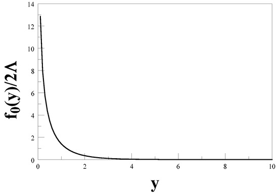
Figure 1.
The distribution function .
It is remarkable that for
in striking contrast to the thermal Fermi–Dirac distribution function. The enhancement for small y indicates that this is a cold dark matter species.
3.2. The Cutoff in the Power Spectrum: Free Streaming Length
The comoving free-streaming wavevector plays the same role as the comoving Jeans wavevector in a fluid, but with the speed of sound replaced by the velocity dispersion of the decoupled particle (see Section 2), it is given by
and its value today is
where
is the three dimensional velocity dispersion of the non-relativistic particles today and we introduced
Using the relation
where is the temperature of the cosmic microwave background today, with is the effective number of relativistic degrees of freedom at decoupling, and for non-baryonic dark matter, leads to
For the non-equilibrium normalized distribution function (75), we find
Taking the number of relativistic degrees of freedom at decoupling (see Equation (71) and preceding discussion), we find
leading to free streaming wavevector and wavelength at matter-radiation equality
For comparison, the value of for a fermion that decoupled with a thermal relativistic relativistic Fermi–Dirac distribution function is
The smaller velocity dispersion in the case of the non-equilibrium distribution function yields a ∼ increase in the free streaming wavevector, and consequently, a decrease in the free streaming length. However, just as importantly in enhancing is decoupling at high temperature for a larger value of . A sterile neutrino produced via the Dodelson–Widrow [21] mechanism at decoupling temperature [21] yields a free streaming wavevector at matter-radiation equality .
4. Production from Standard Model Processes
Sterile neutrinos are weak singlets that do not interact via standard model weak interactions, and couple to the flavor active neutrinos via an off diagonal mass matrix. Different models propose different types of (see-saw like) mass matrices. For our purposes, the only relevant aspect is that the diagonalization of the mass matrix leads to mass eigenstates, and these are ultimately the relevant degrees of freedom that describe dark matter in its various possible realizations, cold, warm or hot. Cold and warm dark matter would be described by heavier species, whereas the usual (light) active-like neutrinos could be a hot dark matter component depending on the absolute value of their masses. In this section, we focus on the production of sterile-like neutrinos from standard model couplings: in the mass basis, neutrinos couple via standard model charged and neutral current interactions, albeit with very small mixing matrix elements. If kinematically allowed, the same processes that produce active neutrinos will produce sterile-like neutrinos with much smaller branching ratios determined by the effective mixing angles.
Upon diagonalization of the mass matrix, the active (massless) flavor neutrino fields are related to the neutrino fields that create/annihilate mass eigenstates as
where , refer to the light (atmospheric, solar) mass eigenstates with massess and refer to sterile-like mass eigenstates of mass .
In the mass basis the full Lagrangian density is
where is the standard model Lagrangian augmented with a diagonal neutrino mass matrix for the active like neutrinos of masses (), in this Lagragian density the charged and neutral interaction vertices are written in terms of the neutrino mass eigenstates with the mixing matrix , is the free field Lagrangian density for the sterile-like neutrinos of masses () and to linear order in
where
with . From now on, we refer to sterile-like neutrinos instead of “sterile” neutrinos, because unlike the concept of a sterile neutrino, the sterile-like mass eigenstates neutrinos do interact with standard model degrees of freedom via charged and neutral current vertices.
In terms of the interaction vertices (90), we can obtain the quantum kinetic equations for production of massive neutrinos to order from the master equation of the form gain–loss described in the previous section, namely
where is the distribution function of the sterile neutrino. This is calculated for each process: the gain term describes the increase in the population by the creation of a sterile-like state and the loss by the annihilation. We first obtain the gain and loss terms in Minkowski space-time, and follow by replacing the respective momenta and temperatures by the physical quantities in the expanding cosmology.
There are important loop corrections at finite temperature, self-energy corrections to the incoming and outgoing external “legs” as well as vertex corrections. There are also finite temperature corrections to the mixing angles arising from self-energy loops, and these tend to suppress the mixing matrix elements [36,37,38,88,89,90]; therefore, in medium the matrix elements and typically in absence of Mikheyev-Smirnov-Wolfenstein (MSW) resonances . At high temperatures, there are hard thermal loop corrections to the self-energy of fermions and vector bosons [91,92,93,94,95,96,97,98,99,100,101,102,103] that lead to novel collective excitations with masses where g is the gauge coupling. Photons and fermion–antifermion pairs form plasmon collective excitations with mass . For , the vector bosons do not acquire a mass via the Higgs mechanism because the ensemble average of the Higgs field vanishes, but they acquire thermal masses akin to the plasmon collective excitations. Thermal masses for collective excitations of could open up kinematic windows for decay into above the electroweak transition.
The quantum kinetic equations from standard model vertices had been obtained in refs. [66,67], and the finite temperature effects on mixing angles and quantum kinetics at the electroweak scale have been studied in refs. [90,104]. Their general form is
where the gain and loss rates are obtained as in Minkowski space time replacing the momenta and energies by the local time dependent counterparts in the expanding cosmology and the (LTE) distribution functions for the various bosonic or fermionic species (with vanishing chemical potentials). As a consequence of the linearity of the quantum kinetic Equation (93), which, in turn is a consequence of keeping only terms of , the full quantum kinetic equation is a simple sum over all possible channels with total gain and loss rates
therefore the gain and loss rates in the quantum kinetic Equation (93) are the total rates (94). For a general discussion of the various standard model processes, see ref. [67], and in refs. [90,104] production from vector boson decay near the electroweak scale was studied in detail, primarily focused on heavier sterile-like neutrinos. These studies revealed novel resonances in absence of lepton asymmetries and unexpected helicity dependence on the production rates. The reader is referred to these articles for further details.
The main point of this discussion is that the final distribution function at decoupling for sterile-like neutrinos is the result of all the kinematically allowed processes that produced these species, hence such distribution function is a mixture of the various production channels.
4.1. Sterile Neutrinos from Pion Decay
It is clear from the discussion above that standard model interaction vertices that lead to the production of active neutrinos will also lead to the production of the sterile-like neutrinos as long as the processes are kinematically allowed. This implies a far broader range of production mechanisms than those that had been the focus in the literature. A reliable calculation of the production rate requires the inclusion of finite temperature corrections to masses and interaction vertices. In this section, we consider the specific example of production of sterile-like neutrinos from pion decay shortly after the QCD phase transition (crossover) into the confined phase.
The QCD phase transition occurs at a temperature scale at a time scale , below quarks and gluons are confined into hadrons, the lightest of which are -mesons (pions). Therefore, these are the degrees of freedom that feature the largest population at temperatures below . Charged pions decay via charged current weak interactions into charged leptons and neutrinos, therefore, as per the discussion in the previous section, this decay process will also contribute to the production of sterile-like neutrinos from the process via the mixing matrix element. In fact, in terrestrial accelerator experiments, charged pion decay is one of the primary sources of neutrinos.
In ref. [40,41,42,43], the authors proposed to study hadronic contributions to the production of sterile neutrinos by considering the self-energy corrections to the active (massless) neutrinos in terms of correlators of vector and axial–vector currents. While this is correct in principle, it is an impractical program: the confined phase of QCD is strongly coupled, and the description in terms of nearly free quarks is at best an uncontrolled simplification, casting doubts on the reliability of the conclusions in this reference.
Instead, in this section, we study the production from pion decay by relying on the well understood effective field theory description of weak interactions of pions, enhanced by the results of a systematic program that studied finite temperature corrections to the pion decay constant and mass implementing non-perturbative techniques from chiral perturbation theory, linear and non-linear sigma models and lattice gauge theory [105,106,107,108,109,110,111,112,113,114,115,116,117,118,119,120]. There are at least three important reasons that motivate this study: (1) it is a clear and relevant example of the quantum kinetic equation approach to production and freeze out that includes consistently finite temperature corrections. (2) Pion decay surely contributed to the production of sterile-like neutrinos in the early universe if such species of neutrinos do exist: the QCD transition to its confined phase undoubtedly happened, and the consequent hadronization resulted in baryons and low lying mesons, pions being the lightest, are the most populated degrees of freedom near the QCD scale. (3) The two leptonic decay channels feature different kinematics and thresholds, in particular the (V-A) vector–axial coupling results in chiral suppression of the e channel for vanishingly small . Since the neutrino produced in the decay is kinematically entangled with the emitted lepton [121], we expect that the distribution functions from each channel will display differences as a manifestation of this kinematic entanglement and dependence on the particular production channel.
At temperatures larger than the QCD phase transition MeV[117,118,119,120], quarks and gluons are asymptotically free. Below this temperature, QCD bound states form on strong interaction time scales, the pion being the lightest. Lattice gauge theory calculations [117,118,119,120] suggest that the confinement–deconfinement transition is not a sharp phase transition, but a smooth yet rapid crossover at a temperature MeV within a temperature range MeV. This occurs in the radiation dominated epoch at s within a time range 2–3 s. This is much larger than the typical strong and electromagnetic interaction time scales s implying that pions that form shortly after the confining cross-over are brought to LTE via strong, electromagnetic and weak interactions on time scales much shorter than . After pions are produced, they reach LTE via scattering on strong interaction time scales, then decay into leptons and maintain LTE via detailed balance with the inverse process since charged leptons and active-like neutrinos are also in LTE. In conclusion, for MeV, pions are present in the plasma in thermal/chemical equilibrium due to pions interacting on strong interaction time scales ( s) while the crossover transition occurs on the order of 2–3 s.
If the pions (slowly) decay into heavy neutrinos with very small mixing angles, detailed balance for will not be maintained if the sterile-like neutrinos are not in LTE. As the pion is the lowest lying bound state of QCD, it is a reasonable assumption that during the QCD confinement–deconfinemet crossover pions will be the most dominantly produced mesonic bound state and, during this time, pions will remain in LTE with the light active-like neutrinos and charged leptons by detailed balance . We focus on sterile-like neutrino production from , which is suppressed by the mixing matrix element with respect to the active neutrinos, and this channel does not maintain detailed balance.
A full study of sterile neutrino production through decay in the early universe requires various finite temperature corrections, and a preliminary study that focused on the production of neutrinos in the mass range [66] has provided a thorough study, the results of which suggest a suitable warm dark matter candidate with free streaming lengths on the order of several kpc. Furthermore, this production mechanism may yield a substantial (if not the dominant) contribution to DM below the QCD scale. We summarize several of these results in this section.
4.2. Quantum Kinetic Equation for
It is generally accepted that in the early universe, where temperatures and densities are larger than the QCD scale (∼155 MeV), quarks and gluons are asymptotically free forming a quark-gluon plasma. As the universe expands and cools, quarks and gluons undergo two phase transitions: deconfinement/confinement and chiral symmetry breaking. Confinement and hadronization result predominantly in the formation of baryons and mesons, the lightest of which—the pions—are dominant and are the pseudo Goldsone bosons associated with chiral symmetry breaking. A recent lattice QCD calculation [117,118,119,120] suggests that this phase transition is not first order but a rapid crossover near a critical temperature MeV. Pions thermalize in the plasma via strong, electromagnetic and weak interactions and are in local thermodynamic equilibrium. Their decay into leptons and active neutrinos is balanced by the inverse process as the leptons and active neutrinos are also in LTE, therefore pions remain in LTE with active neutrinos by detailed balance. However if the pions (slowly) decay into sterile neutrinos, detailed balance will not be maintained, as the latter are not expected to be in LTE.
We focus on sterile neutrino production from , which is suppressed by with respect to the active neutrinos and does not maintain detailed balance. We also restrict the analysis to a scenario with no lepton asymmetry, which sets the chemical potential of pions and leptons to zero. The interaction Hamiltonian responsible for this decay is
where is the pseudoscalar pion current.
The time evolution of the population of sterile-like neutrinos can be described via a quantum kinetic equation that takes the usual form of – where the gain and loss contributions are obtained from the appropriate transition matrix elements obtained from the interaction Hamiltonian (95) (for details see ref. [66]). The quantum kinetic equation is obtained in ref. [66], it is given by
where are the elements of the CKM matrix, is Fermi’s constant, the pion decay constant and are obtained from the constraint
This gives the solutions
Note that these bounds coalesce at when and the rate, Equation (96), vanishes simply because this corresponds to the kinematic threshold. As discussed in the previous section, these results are extended to an expanding cosmology by replacing the momentum with the physical momentum, and the temperature by .
Non-Thermal Sterile Neutrino Distribution Function
A body of work [107,108,109,110,111,112,114,115,116] has established that, when ’s are present in the medium in LTE, the decay constant, , and mass vary with temperature for , where is the critical temperature for the QCD phase transition. We account for these effects and make several simplifications by implementing the following:
- The finite-temperature pion decay constant has been obtained in both non-linear sigma models [108,109,110,111] and Chiral perturbation theory [107,112,114,115,116] with the result given asThis result is required in the quantum kinetic equation since production begins near MeV and continues until the distribution function freezes out. We assume prior to that there are no pions and that hadronization happens instantaneously at MeV.
- The mass of the pion varies with temperature as described in detail in refs. [107,115,116]. The finite temperature corrections to the pion mass is calculated with electromagnetic corrections in chiral perturbation theory and its variation with temperature is shown in Figure 2 of [107]. In these references, it can be seen that between 50 and 150 MeV the pion mass only varies between 140 and 144 MeV. Since this change is so small, we neglect the temperature variation in the pion mass and simply use its average value: MeV (see fig in ref. [107]).
- We assume that the lepton asymmetry in the early universe is very small so that we may neglect the chemical potential in the distribution function of the pions and charged leptons. This asymmetry is required for the Shi–Fuller mechanism, but will not be present in these calculations. We will show a similar enhancement at low moment to SF, but the enhancement found here is with zero lepton asymmetry.
- With the assumption that there is no lepton asymmetry, the contribution to thermodynamic quantities from will be equal to that of . In which case, the degrees of freedom will be set at accounting for both equal particle and antiparticle contributions in the case of Dirac fermions and the two different sources () for Majorana fermions. The different helicities have already been accounted by summing over spins in the evaluation of the matrix elements of the previous section.
- We assume that there had been no production of sterile neutrinos prior to the hadronization period from any other mechanisms (such as scalar decays or DW). This allows us to set the initial distribution of the sterile neutrinos to zero in the kinetic equation, which implies that our results for the distribution function will be a lower bound for the distribution function. Any other prior sources could only enhance the population of sterile neutrinos. By neglecting the initial population, we can neglect the Pauli blocking factor of the ’s in the production term, and we can also neglect the loss term (see discussion below).
After the QCD phase transition, there is an abundance of pions present in the plasma in thermal/chemical equilibrium. The pions will decay, predominantly via , producing sterile neutrinos which, assuming that sterile neutrinos had not been produced up to this point, will have a negligible distribution function. The reverse reaction () will not occur in any significant quantities also due to the assumption of null initial population and ; under these assumptions, we may neglect the loss terms in the kinetic equation. With these assumptions, we use the following distributions for the production terms in the quantum kinetic equation
where is a comoving momentum as discussed in Section 2.
With these replacements, neglecting the loss terms and setting , the quantum kinetic equation becomes
where the limits of integration are given by Equation (98) and we have suppressed the dependence of physical momentum on time. The integral can be done by a simple substitution with the final result given here:
where are given by Equation (98).
Making the following change of variables
where is the temperature of the plasma today since the normalization is set by . The QCD phase transition occurs during the radiation dominated era so that the Hubble factor is given by Equation (51), inserting it into Equation (102) suggests the definition
During the period shortly after hadronization when the relativistic degrees of freedom are while in the regime the degrees of freedom count is [73]. We expect the sterile neutrino decoupling to happen well above the electron mass (this will be justified later) and since the variation of is small we replace it with its average value, , so that we can neglect the time dependence of .
These substitutions and variable changes lead to a more tractable form of the kinetic equation
The population build up is obtained by integrating
where we have neglected any early population of and the value of is determined by when the pions are produced, assumed almost immediately after the hadronization transition. Our assumption is that this happens instantaneous at the QCD phase transition and the pions reach equilibrium instantaneously. This is justified by the results of [117,118,119,120], which suggest a continuous transition that allows for thermalization on strong interaction time scales.
As shown in [117,118,119,120], the continuous phase transition occurs at MeV so that . As we set below this value, we expect that the population would increase, as there will simply be more time for production to occur; this will be confirmed in a subsequent section.
The rate equation and the resulting population buildup as a function of for different values of y has been studied in detail in ref. [66]; however, an estimate of the sterile neutrino decoupling temperature can be made by considering the pion distribution. As the plasma temperature cools to well below the pion mass, the pion distribution will go as , leading to a large suppression of the production rate at MeV, which is when we expect the sterile neutrinos to freeze out. This is indeed what is found numerically in the population build up calculations of ref. [66].
The light mass limit relevant for sterile-like neutrinos with can be studied analytically. As discussed above, we expect freeze out to occur on the order of 10–15 MeV and we will consider here light sterile neutrinos with (MeV). Restricting attention to this mass range sets for the duration of sterile neutrino buildup and simplifies the kinetic equation considerably. For this particular production mechanism, it follows that and we introduce the parameter
so that, upon expanding in small parameters and lead to the following simplifications
which is relevant for a wide range of light steriles that freeze out at . Note that we are suppressing the dependence of and will do so for the remainder of this work (for MeV). In this limit, the kinetic equation simplifies to
We must ensure that the rate remains small in order to ignore the sterile’s population build up and consequent Pauli blocking. The population scales with , and if one were to compute the next order correction by including the first order buildup in the rate equation, the higher order correction would scale as and so on. Provided (discussed below), the first order correction will be sufficient and higher order perturbations will be calculated in future work.
In order to evaluate the integral analytically, several mild simplifications are made. As previously mentioned, we use the fact that varies slowly during the production process and a reasonable estimate is to instead use its average value (12.5). Additionally, if we are restricting our attention to the study of sterile neutrinos with MeV, then the first bracketed term inside of the logarithm (which is independent of ) simplifies considerably.
The remaining dependence in the logarithm is a result of the Bose–Einstein suppression of the pions’ thermal distribution and the dependence is a result of the phase space factors (with 1 MeV).
With these simplifications and by expanding the logarithms in a power series the integral can be carried out analytically. The final result is given as
where is the upper incomplete gamma function.
To get the frozen distribution, we take the long time limit, , to arrive at
Equation (112) is the decoupled distribution function of sterile neutrinos with MeV arising from pion decay near the QCD phase transition. This distribution function is valid for a wide range of sterile neutrino masses as we have only assumed for the period of production/freezeout ( 10–15 MeV), which is valid as long as we consider MeV.
The distribution function is shown for several values of in Figure 2, where it can be seen that decreasing the lower limit increases the value of the distribution function. This is interpreted quite simply: production of steriles begins sooner and so the overall population is larger. If there are pions present in the plasma prior to the hadronization transition, then this could be extended back to temperatures until the finite temperature corrections to the pion decay constant are no longer reliable: .
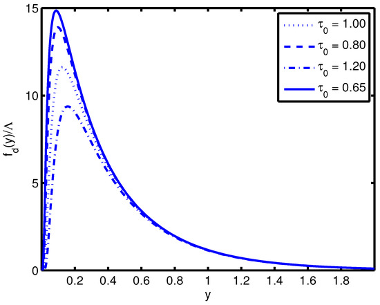
Figure 2.
The distribution function with various values of initial time. Note that an earlier initial time provides an enhancement with respect to later times.
Equation (112) is the decoupled distribution function of sterile neutrinos with 1 MeV arising from pion decay near the QCD phase transition. This distribution function is valid for a wide range of sterile neutrino masses as we have only assumed for the period of production/freezeout ( 10–15 MeV), which is valid as long as we consider 1 MeV.
4.3. Cosmological Consequences
4.3.1. Bounds from Dark Matter and Dwarf Spheroidal Galaxies
The analysis above shows that freezeout occurs between 3–5 or 10–15 MeV, so that sterile-like neutrinos are relativistic at the time of decoupling. For the light sterile neutrinos we consider here, we relate the number of relativistic species at the time of sterile decoupling to the photon temperature today by the usual relation between the plasma and photon temperatures:
For eV, we may neglect terms of , therefore the sterile neutrinos are non-relativistic today yielding
With this, the contribution to the density today is obtained using the distribution function, and we find
where
When MeV the moments, do not vary significantly and, for this mass range, they may be approximated by their value at . We work under the assumption that MeV so that we may use the limit in subsequent calculations, and the limiting values are listed in Table 1.

Table 1.
Table of limiting values for the function .
Using the results of Section 2, if we consider sterile masses with then we may neglect the sterile mass in both so that we arrive at
Considering light scalars simplifies the scales, , so that the appropriate scales in the problem are
so that
Using the values of eV and while assuming and leads to the bounds
As discussed in refs. [9,74,75,76], the dark matter phase space density decreases over the course of galactic evolution and the primordial phase space density may be used as an upper bound to obtain limits on the mass of dark matter. Using observational values for dwarf spheroidal galaxies from ref. [76] a set of bounds complementary to those from CMB measurements can be obtained. As discussed, imposing the condition gives us the constraint
Assuming, as before, that the sterile neutrino mass is much smaller than the charged lepton mass renders the phase space density independent of the sterile neutrino mass. This leads to a bound on the mass given as
Using the results from Section (Section 2), the phase space density is given as
so that the bound becomes
which can serve as a complementary bound to the limits set from . Values of the phase space density today are summarized in ref. [76] and using the data from the most compact dark matter halos leads to bounds on sterile neutrino dark matter. The halo radius (), velocity dispersion (), phase space density today and the calculated bounds are summarized in Table 2 where we chose several of the most compact dwarf spheroidal galaxies (a more thorough list is available in [76]).
Table 2.
Phase space data for compact galaxies and derived bounds on sterile neutrinos arising from pion decay.
Taking the minimum value from this data set translates into the bounds
The analysis of refs. [66,67] suggests that if sterile neutrinos are responsible for the x-ray signal, then production from is a mechanism consistent with the data within a narrow region, while sterile neutrinos produced from are not.
4.3.2. Equation of State and Free Streaming
The equation of state for an arbitrary dark matter candidate is characterized by the parameter . A light sterile neutrino ( MeV) freezes out while it is still relativistic since during production/freezeout; therefore, the results of the previous section hold. This distribution will then determine at what temperature this species becomes non relativistic, which is rewritten here explicitly in terms of :
Many fermionic dark matter candidates that freeze out at temperature are treated as being in LTE in the early universe so that their distribution functions are given by the standard form
To compare the new distribution to thermal results, assume that thermal particles with the same mass also freezeout while relativistic. The equation of state arising from thermal distributions and the non-thermal distribution we obtain are plotted as a function of in Figure 3. Note that the non-thermal distribution equation of state parameter is smaller for all times. This is a reflection of the enhancement of small momentum so that the non-thermal distribution results in a dark matter species, which is colder and becomes non-relativistic much earlier than the thermal result. In summary, the thermal distribution produces particles that become non-relativistic when , whereas the pion decay mechanism produces particles that become non-relativistic when . This non-thermal distribution function produces a dark matter candidate that is colder than those produced at LTE.
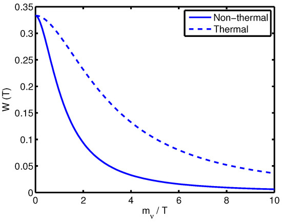
Figure 3.
Equation of state compared to thermal.
The free streaming wavevector enters when one considers a linearized collisionless Bolzmann–Vlasov equation describing the evolution of gravitational perturbations, which ultimately lead towards structure formation [74,75,76,77,78]. The free streaming wavevector leads to a cutoff in the linear power spectrum of density perturbations and is given by
Modes with lead to gravitation collapse in a manner akin to the Jeans instability. This is shown explicitly and discussed at length in refs. [74,75,76]. Assuming that a light sterile neutrino is the only dark matter (so that ) and using the results of Section 2 (for a non-relativistic species), the free streaming wave vector is given by
Using the latest values from Planck [29] sets the free streaming wave vector as
or in terms of the free streaming length, ,
For a redshift z during matter domination the free streaming length scales as and the free streaming length today for the particular processes are then given by
where we have used the notation . These values of the free-streaming length, namely the cutoff in the (DM) power spectrum, are consistent with the size of cores in dwarf galaxies.
Our focus in this study is to bring to the fore alternative production mechanisms of sterile neutrinos and to obtain their frozen distribution function from such processes, and from these their clustering properties for galaxy formation. A further assessment on whether sterile neutrinos produced by a particular mechanism are, indeed, suitable dark matter candidates would require assessing whether their mass range is consistent with the various bounds [122,123].
5. Conclusions
Sterile neutrinos are singlets that do not couple directly to other degrees of freedom, but mix with active neutrinos via a mass matrix. A sterile-like mass eigenstate with a mass scale could be a suitable warm dark matter candidate that could explain various discrepancies between N-body simulations of structure formation with (CDM) and observations of dwarf spheroidal galaxies. In this brief review, we have described alternative production mechanisms of sterile-like neutrinos beyond and within the standard model of particle physics. The main aspects discussed in this review are the following:
- We began with a description of the dynamical properties of dark matter particles described by frozen distribution functions, such as effective equation of state, phase space density and the free-streaming length, which determines the cutoff in the dark matter power spectrum.
- We considered a simple extension beyond the standard model in which sterile-like neutrinos couple to a Higgs-like scalar via a Yukawa coupling, obtaining the quantum kinetic equations for production, the distribution function at freeze out and from it the clustering properties of this (DM) candidate such as the abundance and free streaming length.
- Within the standard model, we have argued that in the basis of mass eigenstates, standard model processes that produce active neutrinos also produce sterile-like neutrinos; however, these are suppressed by the small mixing angles. We discussed several possible production channels, obtained the general form of the quantum kinetic equations to leading order in the mixing angles and analyzed the possibility of thermalization. This analysis leads us to conclude that the final distribution function of sterile-like neutrinos is a result of the various kinematically allowed production processes available during the cosmological history of the early universe.
- As specific example, we focused on the production of sterile-like mass eigenstates from the decay of pions after the QCD phase transition, including finite temperature effects. Shortly after the QCD transition at , s pions being the lightest degrees of freedom in QCD feature large populations and their main decay channels (for charged pions) produce neutrinos. In the basis of mass eigenstates, these processes produce sterile-like neutrinos. We obtained and solved the quantum kinetic equations for production and freeze-out, and from the solution we obtained the clustering properties of sterile-like neutrinos produced via this mechanism. We find that these could be a suitable warm dark matter candidate with the correct abundance if the mass is of the order of few and their free streaming length of a few consistent with the scale of cores in dwarf spheroidal galaxies.
Although direct observational evidence for sterile-like neutrinos remains elusive, these still remain, at least theoretically, as suitable warm dark matter candidates with several possible production channels beyond and within the standard model in the early universe.
Funding
This research received no external funding.
Conflicts of Interest
The author declares no conflict of interest.
References
- Dodelson, S. Modern Cosmology; Academic Press: New York, NY, USA, 2003. [Google Scholar]
- Lesgourgues, J.; Mangano, G.; Miel, G.; Pastor, S. Neutrino Cosmology; Cambridge University Press: Cambridge, MA, USA, 2013. [Google Scholar]
- Cushman, P. Snowmass Summary. arXiv 2013, arXiv:1310.8327. [Google Scholar]
- Kim, J. A review on axions and the strong CP problem. In AIP Conference Proceedings; American Institute of Physics: New York, NY, USA, 2010; Volume 1200, pp. 83–92. [Google Scholar]
- David, J.; Marsh, E. Axion cosmology. Phys. Rep. 2016, 643, 1–79. [Google Scholar]
- Boyarsky, A.; Iakubovskyi, D.; Ruchayskiy, O. Next decade of sterile neutrino studies. Phys. Dark Univ. 2012, 1, 136–154. [Google Scholar] [CrossRef]
- Boyarsky, A.; Ruchayskiy, O.; Shaposhnikov, M. The role of sterile neutrinos in cosmology and astrophysics. Ann. Rev. Nucl. Part. Sci. 2009, 59, 191–214. [Google Scholar] [CrossRef]
- de Blok, W.J.G. The core-cusp problem. Adv. Astron. 2010, 2010, 789293. [Google Scholar] [CrossRef]
- Dalcanton, J.; Hogan, C. Halo cores and phase-space densities: Observational constraints on dark matter physics and structure formation. Astrophys. J. 2001, 561, 35–45. [Google Scholar] [CrossRef]
- Hogan, C.; Dalcanton, J. New dark matter physics: Clues from halo structure. Phys. Rev. D 2000, 62, 063511. [Google Scholar] [CrossRef]
- Boylan-Kolchin, M.; Bullock, J.; Kaplinghat, M. Too big to fail? The puzzling darkness of massive Milky Way subhaloes. Mon. Not. R. Astron. Soc. 2011, 412, L40. [Google Scholar] [CrossRef]
- Garrison-Kimmel, S.; Boylan-Kolchin, M.; Bullock, J.; Kirby, E. Too big to fail in the local group. arXiv 2014, arXiv:1404.5313. [Google Scholar]
- Papastergis, E.; Giovanelli, R.; Haynes, M.; Shankar, F. Is there a “too big to fail” problem in the field? Astron. Astrophys. 2015, 574, A113. [Google Scholar] [CrossRef]
- Walker, M.G.; Penarrubia, J. A method for measuring (slopes of) the mass profiles of dwarf spheroidal galaxies. Astrophys. J. 2011, 20, 742. [Google Scholar] [CrossRef]
- Tikhonov, A.V.; Klypin, A. The emptiness of voids: Yet another overabundance problem for the cold dark matter model. Mon. Not. R. Astron. Soc. 2009, 395, 1915–1924. [Google Scholar] [CrossRef]
- Tikhonov, A.V.; Gottlöber, S.; Yepes, G.; Hoffman, Y. The sizes of minivoids in the local Universe: An argument in favour of a warm dark matter model? Mon. Not. R. Astron. Soc. 2009, 399, 1611–1621. [Google Scholar] [CrossRef]
- Moore, B.; Quinn, T.; Governato, F.; Stadel, J.; Lake, G. Cold collapse and the core catastrophe. Mon. Not. R. Astron. Soc. 1999, 310, 1147–1152. [Google Scholar] [CrossRef]
- Bode, P.; Ostriker, J.P.; Turok, N. Halo formation in warm dark matter models. Astrophys. J. 2001, 556, 93. [Google Scholar] [CrossRef]
- Avila-Reese, V.; Colín, P.; Valenzuela, O.; D’Onghia, E.; Firmani, C. Formation and structure of halos in a warm dark matter cosmology. Astrophys. J. 2001, 559, 516. [Google Scholar] [CrossRef]
- Lovell, M.R.; Frenk, C.S.; Eke, V.R.; Jenkins, A.; Gao, L.; Theuns, T. The properties of warm dark matter haloes. Mon. Not. R. Astron. Soc. 2014, 439, 300–317. [Google Scholar] [CrossRef]
- Dodelson, S.; Widrow, L.M. Sterile neutrinos as dark matter. Phys. Rev. Lett. 1994, 72, 17–20. [Google Scholar] [CrossRef]
- Simonetti, J.H.; Dennison, B.; Topasna, G.A. The Contribution Of Galactic Free-Free Emission to Anisotropies in the Cosmic Microwave Background Found by the Saskatoon Experiment. Astrophys. J. Lett. 1996, 458, L1. [Google Scholar] [CrossRef]
- Abazajian, K.; Fuller, G.M.; Patel, M. Sterile neutrino hot, warm, and cold dark matter. Phys. Rev. D 2001, 64, 023501. [Google Scholar] [CrossRef]
- Abazajian, K.N.; Acero, M.A.; Agarwalla, S.K.; Aguilar-Arevalo, A.A.; Albright, C.H.; Antusch, S.; Marfatia, D. Light sterile neutrinos: A white paper. arXiv 2012, arXiv:1204.5379. [Google Scholar]
- Chialva, D.; Dev, P.B.; Mazumdar, A. Multiple dark matter scenarios from ubiquitous stringy throats. Phys. Rev. D 2013, 87, 063522. [Google Scholar] [CrossRef]
- Paduroiu, S.; Revaz, Y.; Pfenniger, D. Structure formation in warm dark matter cosmologies: Top-Bottom Upside-Down. arXiv 2015, arXiv:1506.03789. [Google Scholar]
- Maccio, A.V.; Paduroiu, S.; Anderhalden, D.; Schneider, A.; Moore, B. Cores in warm dark matter haloes: A Catch 22 problem. Mon. Not. R. Astron. Soc. 2012, 424, 1105. [Google Scholar] [CrossRef]
- Shao, S.; Gao, L.; Theuns, T.; Frenk, C. The phase-space density of fermionic dark matter haloes. Mon. Not. R. Astron. Soc. 2013, 430, 2346. [Google Scholar] [CrossRef]
- Ade, P.A.; Aghanim, N.; Armitage-Caplan, C.; Arnaud, M.; Ashdown, M.; Atrio-Barandela, F.; Meinhold, P.R. Planck 2013 results. XVI. Cosmological parameters. Astron. Astrophys. 2014, 571, A16. [Google Scholar]
- Barbieri, R.; Dolgov, A.D. Neutrino oscillations in the early universe. Nucl. Phys. B 1991, 349, 743–753. [Google Scholar] [CrossRef]
- Barbieri, R.; Dolgov, A.D. Bounds on sterile neutrinos from nucleosynthesis. Phys. Lett. 1990, B237, 440–445. [Google Scholar] [CrossRef]
- Kainulainen, K. Light singlet neutrinos and the primordial nucleosynthesis. Phys. Lett. B 1990, 244, 191–195. [Google Scholar] [CrossRef]
- Enqvist, K.; Kainulainen, K.; Maalampi, J. Resonant neutrino transitions and nucleosynthesis. Phys. Lett. B 1990, 249, 531–534. [Google Scholar] [CrossRef]
- Enqvist, K.; Kainulainen, K.; Maalampi, J. Refraction and oscillations of neutrinos in the early universe. Nucl. Phys. B 1991, 349, 754–790. [Google Scholar] [CrossRef]
- Enqvist, K.; Kainulainen, K.; Thomson, M. Stringent cosmological bounds on inert neutrino mixing. Nucl. Phys. B 1992, 373, 498–528. [Google Scholar] [CrossRef]
- Dolgov, A.D. Neutrinos in cosmology. Phys. Rep. 2002, 370, 333. [Google Scholar] [CrossRef]
- Dolgov, A.D. Cosmology and neutrino properties. Phys. Atom. Nucl. 2008, 71, 2152. [Google Scholar] [CrossRef][Green Version]
- Dolgov, A.D. Cosmological implications of neutrinos. Surv. High Energy Phys. 2002, 17, 91. [Google Scholar] [CrossRef][Green Version]
- Shi, X.; Fuller, G.M. New dark matter candidate: Nonthermal sterile neutrinos. Phys. Rev. Lett. 1999, 82, 2832. [Google Scholar] [CrossRef]
- Asaka, T.; Laine, M.; Shaposhnikov, M. Lightest sterile neutrino abundance within the νMSM. J. High Energy Phys. 2007, 0701, 091. [Google Scholar] [CrossRef]
- Asaka, T.; Laine, M.; Shaposhnikov, M. On the hadronic contribution to sterile neutrino production. J. High Energy Phys. 2006, 0606, 053. [Google Scholar] [CrossRef]
- Asaka, T.; Shaposhnikov, M.; Kusenko, A. Opening a new window for warm dark matter. Phys. Lett. B 2006, 638, 401. [Google Scholar] [CrossRef]
- Asaka, T.; Shaposhnikov, M. The νMSM, dark matter and baryon asymmetry of the universe. Phys. Lett. B 2005, 620, 17. [Google Scholar] [CrossRef]
- Ghisoiu, I.; Laine, M. Right-handed neutrino production rate at T > 160 GeV. J. Cosmol. Astron. Phys. 2014, 1412, 032. [Google Scholar] [CrossRef]
- Laine, M.; Shaposhnikov, M. Sterile neutrino dark matter as a consequence of νMSM-induced lepton asymmetry. J. Cosmol. Astron. Phys. 2008, 0806, 031. [Google Scholar] [CrossRef]
- Venumadhav, T.; Cyr-Racine, F.Y.; Abazajian, K.N.; Hirata, C.M. Sterile neutrino dark matter: A tale of weak interactions in the strong coupling epoch. arXiv 2015, arXiv:1507.06655. [Google Scholar] [CrossRef]
- Boyanovsky, D. Clustering properties of a sterile neutrino dark matter candidate. Phys. Rev. D 2008, 78, 103505. [Google Scholar] [CrossRef]
- Petraki, K.; Kusenko, A. Dark-matter sterile neutrinos in models with a gauge singlet in the Higgs sector. Phys. Rev. D 2008, 77, 065014. [Google Scholar] [CrossRef]
- Petraki, K. Small-scale structure formation properties of chilled sterile neutrinos as dark matter. Phys. Rev. D 2008, 77, 105004. [Google Scholar] [CrossRef]
- Merle, A. keV neutrino model building. Int. J. Mod. Phys. D 2013, 22, 1330020. [Google Scholar] [CrossRef]
- Merle, A.; Schneider, A. Production of sterile neutrino dark matter and the 3.5 keV line. arXiv 2015, arXiv:1409.6311. [Google Scholar] [CrossRef]
- Merle, A.; Totzauer, M. keV sterile neutrino dark matter from singlet scalar decays: Basic concepts and subtle features. J. Cosmol. Astron. Phys. 2015, 6, 011. [Google Scholar] [CrossRef][Green Version]
- Merle, A.; Niro, V.; Schmidt, D. New production mechanism for keV sterile neutrino dark matter by decays of frozen-in scalars. J. Cosmol. Astron. Phys. 2014, 1403, 028. [Google Scholar] [CrossRef]
- Watson, C.R.; Li, Z.; Polley, N.K. Constraining sterile neutrino warm dark matter with Chandra observations of the Andromeda galaxy. J. Cosmol. Astron. Phys. 2012, 3, 018. [Google Scholar] [CrossRef]
- Yuksel, H.; Beacom, J.F.; Watson, C.R. Strong upper limits on sterile neutrino warm dark matter. Phys. Rev. Lett. 2008, 101, 121301. [Google Scholar] [CrossRef]
- Bulbul, E.; Markevitch, M.; Foster, A.; Smith, R.; Loewenstein, M.; Randall, S. Detection of an unidentified emission line in the stacked X-ray spectrum of galaxy clusters. Astrophys. J. 2014, 13, 789. [Google Scholar] [CrossRef]
- Boyarsky, A.; Ruchayskiy, O.; Iakubovskyi, D.; Franse, J. Unidentified line in X-ray spectra of the Andromeda galaxy and Perseus galaxy cluster. arXiv 2014, arXiv:1402.4119. [Google Scholar] [CrossRef]
- Boyarsky, A.; Franse, J.; Iakubovskyi, D.; Rucharyskiy, O. Checking the dark matter origin of a 3.53 keV line with the Milky Way center. Phys. Rev. Lett. 2015, 115, 161301. [Google Scholar] [CrossRef] [PubMed]
- Jeltema, T.; Profumo, S. Discovery of a 3.5 keV line in the Galactic Centre and a critical look at the origin of the line across astronomical targets. Mon. Not. R. Astron. Soc. 2015, 450, 2143. [Google Scholar] [CrossRef]
- Jeltema, T.; Profumo, S. Reply to Two Comments on “Dark matter searches going bananas the contribution of Potassium (and Chlorine) to the 3.5 keV line”. arXiv 2014, arXiv:1411.1759. [Google Scholar]
- Malyshev, D.; Neronov, A.; Eckert, D. Constraints on 3.55 keV line emission from stacked observations of dwarf spheroidal galaxies. Phys. Rev. D 2014, 90, 103506. [Google Scholar] [CrossRef]
- Abazajian, K. Resonantly produced 7 keV sterile neutrino dark matter models and the properties of Milky Way satellites. Phys. Rev. Lett. 2014, 112, 161303. [Google Scholar] [CrossRef] [PubMed]
- Abazajian, K.N.; Fuller, G.M. Bulk QCD thermodynamics and sterile neutrino dark matter. Phys. Rev. D 2002, 66, 023526. [Google Scholar] [CrossRef]
- Horiuchi, S.; Humphrey, P.J.; Onorbe, J.; Abazajian, K.N.; Kaplinghat, M.; Garrison-Kimmel, S. Sterile neutrino dark matter bounds from galaxies of the Local Group. Phys. Rev. D 2014, 89, 025017. [Google Scholar] [CrossRef]
- Kaplinghat, M.; Lopez, R.E.; Dodelson, S.; Scherrer, R.J. Improved treatment of cosmic microwave background fluctuations induced by a late-decaying massive neutrino. Phys. Rev. D 1999, 60, 123508. [Google Scholar] [CrossRef]
- Lello, L.; Boyanovsky, D. Cosmological implications of light sterile neutrinos produced after the QCD phase transition. Phys. Rev. D 2015, 91, 063502. [Google Scholar] [CrossRef]
- Lello, L.; Boyanovsky, D. The case for mixed dark matter from sterile neutrinos. J. Cosmol. Astron. Phys. 2016, 6, 011. [Google Scholar] [CrossRef][Green Version]
- Ng, K.C.; Horiuchi, S.; Gaskins, J.M.; Smith, M.; Preece, R. Improved limits on sterile neutrino dark matter using full-sky Fermi Gamma-ray Burst Monitor data. Phys. Rev. D 2015, 92, 043503. [Google Scholar] [CrossRef]
- De Vega, H.J.; Salucci, P.; Sanchez, N.G. The mass of the dark matter particle: Theory and galaxy observations. New Astron. 2012, 17, 653. [Google Scholar] [CrossRef]
- De Vega, H.J.; Sanchez, N.G. Model-independent analysis of dark matter points to a particle mass at the keV scale. Mon. Not. R. Astron. Soc. 2010, 404, 885. [Google Scholar] [CrossRef]
- Merle, A.; Schneider, A.; Totzauer, M. Dodelson-Widrow production of sterile neutrino dark matter with non-trivial initial abundance. J. Cosmol. Astron. Phys. 2016, 4, 003. [Google Scholar] [CrossRef]
- Bernstein, J. Kinetic Theory in the Expanding Universe; Cambridge University Press: Cambridge, MA, USA, 1988. [Google Scholar]
- Kolb, E.W.; Turner, M.S. The Early Universe; Addison-Wesley: Boston, MA, USA, 1990. [Google Scholar]
- Boyanovsky, D.; De Vega, H.J.; Sanchez, N.G. Constraints on dark matter particles from theory, galaxy observations, and N-body simulations. Phys. Rev. D 2008, 77, 043518. [Google Scholar] [CrossRef]
- Boyanovsky, D.; De Vega, H.J.; Sanchez, N.G. Dark matter transfer function: Free streaming, particle statistics, and memory of gravitational clustering. Phys. Rev. D 2008, 78, 063546. [Google Scholar] [CrossRef]
- Destri, C.; De Vega, H.J.; Sanchez, N.G. Warm dark matter primordial spectra and the onset of structure formation at redshift z. Phys. Rev. D 2013, 88, 083512. [Google Scholar] [CrossRef]
- De Vega, H.J.; Sanchez, N.G. Cosmological evolution of warm dark matter fluctuations. I. Efficient computational framework with Volterra integral equations. Phys. Rev. D 2012, 85, 043516. [Google Scholar] [CrossRef]
- De Vega, H.J.; Sanchez, N.G. Cosmological evolution of warm dark matter fluctuations. II. Solution from small to large scales and keV sterile neutrinos. Phys. Rev. D 2012, 85, 043517. [Google Scholar] [CrossRef]
- Boyanovsky, D.; Wu, J. Small scale aspects of warm dark matter: Power spectra and acoustic oscillations. Phys. Rev. D 2011, 83, 043524. [Google Scholar] [CrossRef]
- Lee, B.W.; Weinberg, S. Cosmological lower bound on heavy-neutrino masses. Phys. Rev. Lett. 1977, 39, 165. [Google Scholar] [CrossRef]
- Hut, P. Limits on masses and number of neutral weakly interacting particles. Phys. Lett. 1977, B69, 85. [Google Scholar] [CrossRef]
- Sato, K.; Kobayashi, H. Cosmological constraints on the mass and the number of heavy lepton neutrinos. Prog. Theor. Phys. 1977, 58, 1775. [Google Scholar] [CrossRef]
- Vysotsky, M.I.; Dolgov, A.D.; Zeldovich, Y.B. Cosmological restriction on neutral lepton masses. JETP Lett. 1977, 26, 188. [Google Scholar]
- Cowsik, R.; McClelland, J. An upper limit on the neutrino rest mass. Phys. Rev. Lett. 1972, 29, 669. [Google Scholar] [CrossRef]
- Tremaine, S.; Gunn, J.E. Dynamical role of light neutral leptons in cosmology. Phys. Rev. Lett. 1979, 42, 407. [Google Scholar] [CrossRef]
- Kusenko, A. Sterile neutrinos, dark matter, and pulsar velocities in models with a Higgs singlet. Phys. Rev. Lett. 2006, 97, 241301. [Google Scholar] [CrossRef] [PubMed]
- Shaposhnikov, M.; Tkachev, I. The vMSM, inflation, and dark matter. Phys. Lett. 2006, B639, 414. [Google Scholar] [CrossRef]
- Notzold, D.; Raffelt, G. Neutrono dispersion at finite temperature and density. Nucl. Phys. B 1988, 307, 924. [Google Scholar] [CrossRef]
- Pal, P.B.; Pham, T.N. Field-theoretic derivation of Wolfenstein’s matter-oscillation formula. Phys. Rev. D 1989, 40, 259. [Google Scholar] [CrossRef]
- Wu, J.; Ho, C.M.; Boyanovsky, D. Sterile neutrinos produced near the electroweak scale: Mixing angles, MSW resonances, and production rates. Phys. Rev. D 2009, 80, 103511. [Google Scholar] [CrossRef]
- Weldon, H.A. Covariant calculations at finite temperature: The relativistic plasma. Phys. Rev. D 1982, 26, 1394. [Google Scholar] [CrossRef]
- Braaten, E.; Pisarski, R. Soft amplitudes in hot gauge theories: A general analysis. Nucl. Phys. B 1990, 337, 569. [Google Scholar] [CrossRef]
- Braaten, E.; Pisarski, R. Deducing hard thermal loops from Ward identities. Nucl. Phys. B 1990, 339, 310. [Google Scholar] [CrossRef]
- Braaten, E.; Pisarski, R. Resummation and gauge invariance of the gluon damping rate in hot QCD. Phys. Rev. Lett. 1990, 64, 1338. [Google Scholar] [CrossRef] [PubMed]
- Braaten, E.; Pisarski, R. Calculation of the gluon damping rate in hot QCD. Phys. Rev. D 1990, 42, 2156. [Google Scholar] [CrossRef]
- Braaten, E.; Pisarski, R. Simple effective Lagrangian for hard thermal loops. Phys. Rev. D 1992, 45, 1827. [Google Scholar] [CrossRef]
- Braaten, E.; Pisarski, R. Calculation of the quark damping rate in hot QCD. Phys. Rev. D 1992, 46, 1829. [Google Scholar] [CrossRef] [PubMed]
- Pisarski, R. Effective Lagrangian at high temperature. Nucl. Phys. A 1992, 554, 527C. [Google Scholar] [CrossRef]
- Pisarski, R. Medley in finite temperature field theory. Can. J. Phys. 1993, 71, 280. [Google Scholar] [CrossRef]
- Pisarski, R. Scattering Amplitudes in Hot Gauge Theories. Phys. Rev. Lett. 1989, 63, 1129. [Google Scholar] [CrossRef] [PubMed]
- Pisarski, R. How to Compute Scattering Amplitudes in Hot Gauge Theories. Physica A 1989, 158, 246. [Google Scholar] [CrossRef]
- Frenkel, J.; Taylor, J.C. High-temperature limit of thermal QCD. Nucl. Phys. B 1990, 334, 199. [Google Scholar] [CrossRef]
- Le Bellac, M. Thermal Field Theory; Cambridge Monographs on Mathematical Physics; Cambridge University Press: Cambridge, MA, USA, 1996. [Google Scholar]
- Lello, L.; Boyanovsky, D.; Pisarski, R.D. Production of heavy sterile neutrinos from vector boson decay at electroweak temperatures. Phys. Rev. D 2017, 95, 043524. [Google Scholar] [CrossRef]
- Boyanovsky, D.; De Vega, H.J.; Wang, S.Y. Nonequilibrium pion dynamics near the critical point in a constituent quark model. Nucl. Phys. A 2004, 741, 323. [Google Scholar] [CrossRef][Green Version]
- Rajagopal, K.; Wilczek, F. Emergence of coherent long wavelength oscillations after a quench: Application to QCD. Nucl. Phys. 1993, B404, 577. [Google Scholar] [CrossRef]
- Nicola, A.G.; Andrés, R.T. Electromagnetic effects in the pion dispersion relation at finite temperature. Phys. Rev. 2014, D89, 116009. [Google Scholar]
- Pisarski, R.D.; Tytgat, M.H.G. pi0–> gamma gamma and the axial anomaly at non zero temperature. arXiv 1997, arXiv:hepph/9705316. [Google Scholar]
- Pisarski, R.D.; Tytgat, M.H.G. Scattering of soft, cool pions. Phys. Rev. Lett. 1997, 78, 3622. [Google Scholar] [CrossRef]
- Pisarski, R.D.; Tytgat, M.H.G. Propagation of cool pions. Phys. Rev. D 1996, 54, 2989–2993. [Google Scholar] [CrossRef]
- Pisarski, R.D.; Trueman, T.L.; Tytgat, M.H.G. How π0→γγ changes with temperature. Phys. Rev. D 1997, 56, 7077. [Google Scholar] [CrossRef]
- Jeon, S.; Kapusta, J. Pion decay constant at finite temperature in the nonlinear model. Phys. Rev. D 1996, 54, 6475–6478. [Google Scholar] [CrossRef] [PubMed]
- Dominguez, C.A.; Fetea, M.S.; Loewe, M. Pions at finite temperature from QCD sum rules. Phys. Lett. B 1996, 387, 151. [Google Scholar] [CrossRef]
- Harada, M.; Shibata, A. Pion decay constant and the meson mass at finite temperature in hidden local symmetry. Phys. Rev. D 1997, 55, 6716. [Google Scholar] [CrossRef]
- Nicola, A.G.; Fernandez-Fraile, D. Chiral symmetry and mesons in hot and dense matter: Recent developments. arXiv 2010, arXiv:1011.3920. [Google Scholar]
- Toublan, D. Pion dynamics at finite temperature. Phys. Rev. D 1997, 56, 5629. [Google Scholar] [CrossRef]
- Bhattacharya, T. The QCD phase transition with physical-mass, chiral quarks. Phys. Rev. Lett. 2014, 113, 082001. [Google Scholar] [CrossRef] [PubMed]
- Bazavov, A. Equation of state in (2+1)-flavor QCD. Phys. Rev. D 2014, 90, 094503. [Google Scholar] [CrossRef]
- Bazavov, A. Chiral and deconfinement aspects of the QCD transition. Phys. Rev. D 2012, 85, 054503. [Google Scholar] [CrossRef]
- Bazavov, A. Equation of state and QCD transition at finite temperature. Phys. Rev. D 2009, 80, 014504. [Google Scholar] [CrossRef]
- Lello, L.; Boyanovsky, D. Searching for sterile neutrinos from and K decays. Phys. Rev. D 2013, 87, 073017. [Google Scholar] [CrossRef]
- Aviles, A.; Banerjee, A. A Lagrangian Perturbation Theory in the presence of massive neutrinos. J. Cosmol. Astron. Phys. 2020, 10, 034. [Google Scholar] [CrossRef]
- Lesgourgues, J.; Pastor, S. Massive neutrinos and cosmology. Phys. Rep. 2006, 429, 307–379. [Google Scholar] [CrossRef]
Publisher’s Note: MDPI stays neutral with regard to jurisdictional claims in published maps and institutional affiliations. |
© 2021 by the author. Licensee MDPI, Basel, Switzerland. This article is an open access article distributed under the terms and conditions of the Creative Commons Attribution (CC BY) license (https://creativecommons.org/licenses/by/4.0/).