New Model of 4D Einstein–Gauss–Bonnet Gravity Coupled with Nonlinear Electrodynamics

Abstract

New spherically symmetric solution in 4D Einstein–Gauss–Bonnet gravity coupled with nonlinear electrodynamics is obtained. At infinity, this solution has the Reissner–Nordström behavior of the charged black hole. The black hole thermodynamics, entropy, shadow, energy emission rate, and quasinormal modes of black holes are investigated.

1. Introduction

The heterotic string theory at the low energy limit gives the action including higher order curvature terms [1,2,3,4,5]. Glavan and Lin proposed a new theory of gravity in four dimensions, 4D Einstein–Gauss–Bonnet gravity (4D EGB) [6], with higher-order curvature corrections. The action of the 4D EGB theory consists of the Einstein–Hilbert action and the Gauss–Bonnet (GB) term, which is a case of the Lovelock theory. The Lovelock gravity represents the generalization of Einstein’s general relativity in higher dimensions that leads to covariant second-order field equations. The Einstein–Gauss–Bonnet gravity in 5D and higher dimensions was studied in [7]. Recently, 4D EGB gravity has received much attention [8,9,10,11,12,13,14,15,16,17,18,19,20,21,22,23,24,25,26,27]. Glavan and Lin showed [6] that the GB term, which is a topological invariant before regularization, while rescaling the coupling constant after regularization, contributes to the equation of motion. The authors of [12,13] found a solution of the semiclassical Einstein equations with conformal anomaly, which is also a solution in the 4D EGB gravity. The approach of Glavan and Lin was recently debated in [28,29,30,31,32,33]. It was shown by [34,35] that solutions in the 4D EGB theory are different from GR solutions as they are due to extra infinitely strongly coupled scalars. The authors of [36,37,38] proposed a consistent theory of 4D EGB gravity with two dynamical degrees of freedom that breaks the temporal diffeomorphism invariance, in agreement with the Lovelock theorem. In accordance with the Lovelock theorem [11], for a novel 4D theory with two degrees of freedom, the 4D diffeomorphism invariance has to be broken. In the theory of [36,37,38], the invariance under the 3D spatial diffeomorphism holds. The authors considered EGB gravity in arbitrary D-dimensions with the Arnowitt–Deser–Misner decomposition. Then, they regularized the Hamiltonian with counterterms, where $D-1$ diffeomorphism invariance holds and taking the limit $D\to 4$. It should be noted that the theory of [36,37,38], in the spherically symmetric metrics, represents the solution that is a solution in the scheme of [6] (see [39]). In this work, we obtain a black hole (BH) solution in the 4D EGB gravity coupled with nonlinear electrodynamics (NED) proposed in [40] in the framework of [36,37,38] theory. Quasinormal modes, deflection angle, shadows of BHs, and Hawking radiation were studied in [41,42,43,44,45,46,47]. The image of the M87* BH, observed by collaboration with the Event Horizon Telescope [48], confirms the existence of BHs in the universe. The BH shadow is the closed curve that separates capture orbits and scattering orbits. For a review on BH shadows, see, for example, [49].

The paper is organized as follows. In Section 2, we find BH spherically symmetric solution in the 4D EGB gravity. It is shown that at infinity, we have the Reissner–Nordström behavior of the charged BH. We study the BH thermodynamics in Section 3. The Hawking temperature and the heat capacity are calculated showing the possibility of second-order phase transitions. The entropy of BHs is obtained, which includes the area law and the logarithmic correction. In Section 4, the BH shadow is studied. The photon sphere radii, the event horizon radii, and the shadow radii are calculated. We investigate the BH energy emission rate in Section 5. In Section 6, quasinormal modes are studied, and we obtain the complex frequencies. In Section 7, we draw our conclusions.

2. The Model

The action of the EGB gravity in D-dimensions coupled with nonlinear electrodynamics (NED) is given by

$$I=\int d^{D}x\sqrt{-g}\left[\frac{1}{16\pi G}\left(R+\alpha {\mathcal{L}}_{GB}\right)+{\mathcal{L}}_{NED}\right],$$

(1)

where $\alpha$ has the dimension of (length)${}^2$, and the Lagrangian of NED, proposed in [40], is

$${\mathcal{L}}_{NED}=-\frac{\mathcal{F}}{cosh\left(\sqrt[4]{\left|\beta \mathcal{F}\right|}\right)},$$

(2)

with the parameter $\beta$ ($\beta \ge 0$) having the dimension of (length)${}^4$, $\mathcal{F}=(1/4)F_{\mu \nu }{F}^{\mu \nu }=(B^2-E^2)/2$, $F_{\mu \nu }={\partial }_{\mu }{A}_{\nu }-{\partial }_{\nu }{A}_{\mu }$ is the field strength tensor. The GB Lagrangian reads

$${\mathcal{L}}_{GB}=R^{\mu \nu \alpha \beta }{R}_{\mu \nu \alpha \beta }-4R^{\mu \nu }{R}_{\mu \nu }+R^2.$$

(3)

The variation of action (1) with respect to the metric results in field equations

$$R_{\mu \nu }-\frac{1}{2}{g}_{\mu \nu }R+\alpha H_{\mu \nu }=-8\pi G{T}_{\mu \nu },$$

(4)

where

$$H_{\mu \nu }=2\left(R{R}_{\mu \nu }-2R_{\mu \alpha }{R}_{\nu }^{\alpha }-2R_{\mu \alpha \nu \beta }{R}^{\alpha \beta }-R_{\mu \alpha \beta \gamma }{R}_{\nu }^{\alpha \beta \gamma }\right)-\frac{1}{2}{\mathcal{L}}_{GB}{g}_{\mu \nu }.$$

(5)

In the following we consider a magnetic BH with the spherically symmetric field. The static and spherically symmetric metric in D dimension is given by

$$d{s}^2=-f\left(r\right)d{t}^2+\frac{d{r}^2}{f\left(r\right)}+r^{2}d{\Omega }_{D-2}^2,$$

(6)

where $d{\Omega }_{D-2}^2$ is the line element of the unit $(D-2)$-dimensional sphere. Equations (1) and (3)–(5) are valid in D dimensions, and we will consider rescaled $\alpha$ as $\alpha \to \alpha /(D-4)$ and then the limit $D\to 4$. Taking into account that the electric charge $q_e=0$, $\mathcal{F}=q^2/\left(2r^4\right)$ (q is a magnetic charge), one obtains the magnetic energy density [40]

$$\rho =T_0^0=-\mathcal{L}=\frac{\mathcal{F}}{cosh\left(\sqrt[4]{\left|\beta \mathcal{F}\right|}\right)}=\frac{1}{\beta x^{4}cosh\left(1/x\right)},$$

(7)

where we introduced the dimensionless variable $x=2^{1/4}r/\left({\beta }^{1/4}\sqrt{q}\right)$. We consider the limit $D\to 4$ and at $\mu =\nu =t$ field Equation (4) gives

$$r(2\alpha f\left(r\right)-r^2-2\alpha )f^{\prime }\left(r\right)-(r^2+\alpha f\left(r\right)-2\alpha )f\left(r\right)+r^2-\alpha =2r^{4}G\rho .$$

(8)

Making use of Equation (7), we obtain

$${\int }_0^r{r}^2\rho dr=m_M-\frac{2^{1/4}{q}^{3/2}}{{\beta }^{1/4}}arctan\left(tanh\left(\frac{{\beta }^{1/4}\sqrt{q}}{2^{5/4}r}\right)\right),$$

(9)

where the magnetic mass of the black hole reads

$$m_M={\int }_0^{\infty }{r}^2\rho dr=\frac{\pi q^{3/2}}{2^{7/4}{\beta }^{1/4}}.$$

(10)

Then, the solution to Equation (8) is

$$f\left(r\right)=1+\frac{r^2}{2\alpha }\left(1\pm \sqrt{1+\frac{8\alpha G}{r^3}(m+h\left(r\right))}\right),$$

$$h\left(r\right)=m_M-\frac{2^{1/4}{q}^{3/2}}{{\beta }^{1/4}}arctan\left(tanh\left(\frac{{\beta }^{1/4}\sqrt{q}}{2^{5/4}r}\right)\right),$$

(11)

where m is the Schwarzschild mass (the constant of integration), and $M=m+m_M$ is the total mass of the BH. One can verify that the Weyl tensor for the D-dimensional spatial part of the spherically symmetric D-dimensional line element (6) vanishes [39]. As a result, the new solution (11) obtained in the framework of [6] is also a solution for the consistent theory [36,37,38]. For Maxwell electrodynamics, the energy density is $\rho =q^2/\left(2r^4\right)$, and Equation (8) leads to the metric function obtained in [15]. In the dimensionless form, Equation (11) becomes

$$f\left(x\right)=1+C{x}^2\pm C\sqrt{x^4+x(A-Bg\left(x\right))},$$

(12)

where

$$A=\frac{2^{15/4}(m+m_M)\alpha G}{{\beta }^{3/4}{q}^{3/2}},B=\frac{16\alpha G}{\beta },C=\frac{\sqrt{\beta }q}{2\sqrt{2}\alpha },$$

$$g\left(x\right)=arctan\left(tanh\left(\frac{1}{2x}\right)\right),$$

(13)

We will use the sign minus of the square root in Equations (11) and (12) (the negative branch) because, in this case, the BH is stable and without ghosts [8]. The asymptotic of the metric function $f\left(r\right)$ (11) for the negative branch is given by

$$f\left(r\right)=1-\frac{2MG}{r}+\frac{G{q}^2}{r^2}+\mathcal{O}\left(r^{-3}\right)r\to \infty ,$$

(14)

where the total mass of the BH $M=m+m_M$ includes the Schwarzschild mass m and the electromagnetic mass $m_M$. According to Equation (14), the Reissner−Nordström behavior of the charged BH holds at infinity. It is worth noting that the limit $\beta \to 0$ has been in Equation (8) before the integration. In this case, the solution to Equation (8) at $\beta =0$ is given by [15]. The plot of the function (12) is given in Figure 1.

In accordance with Figure 1,we have two horizons—one (the extreme) horizon and no horizons—depending on the model parameters.

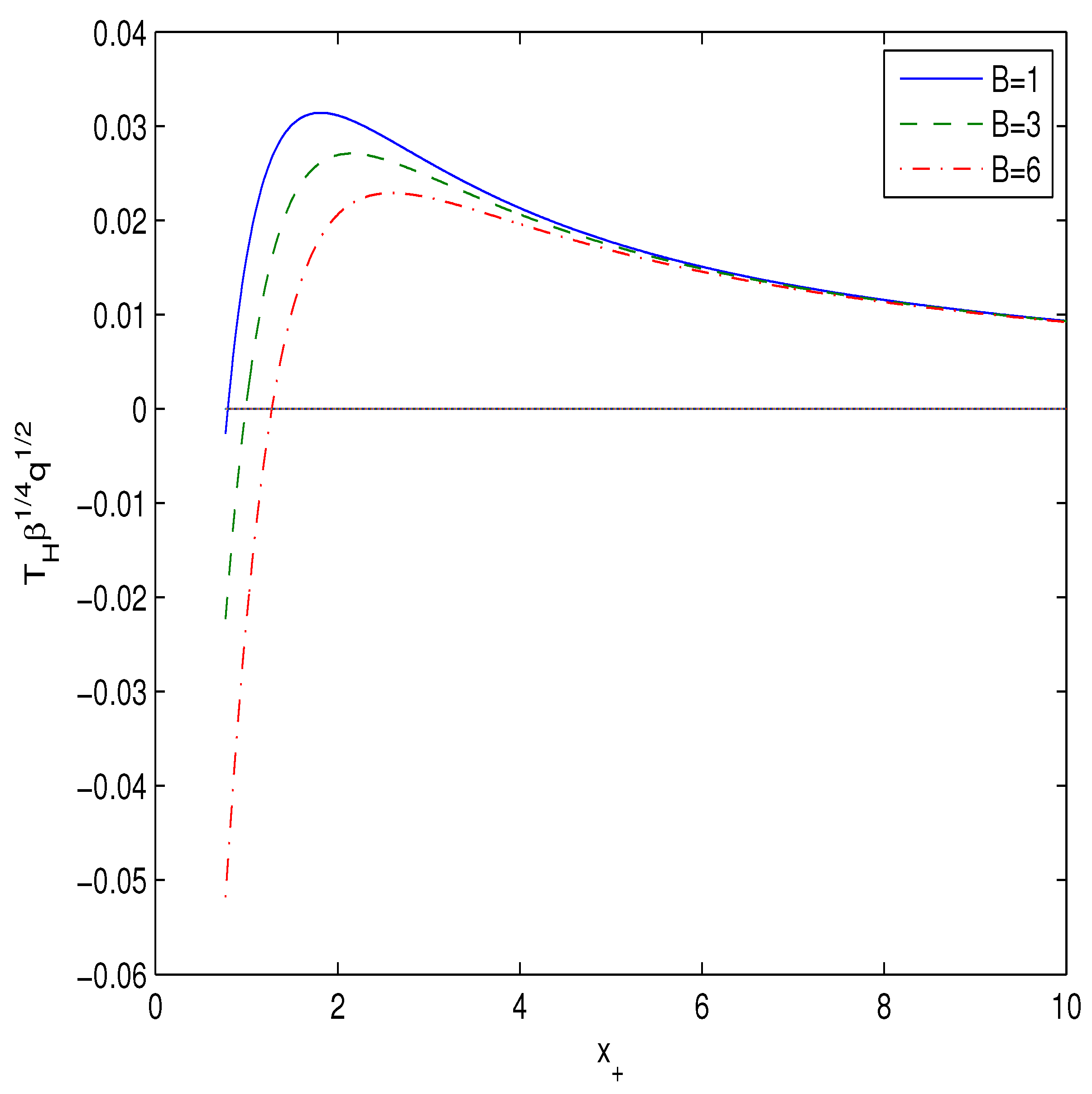
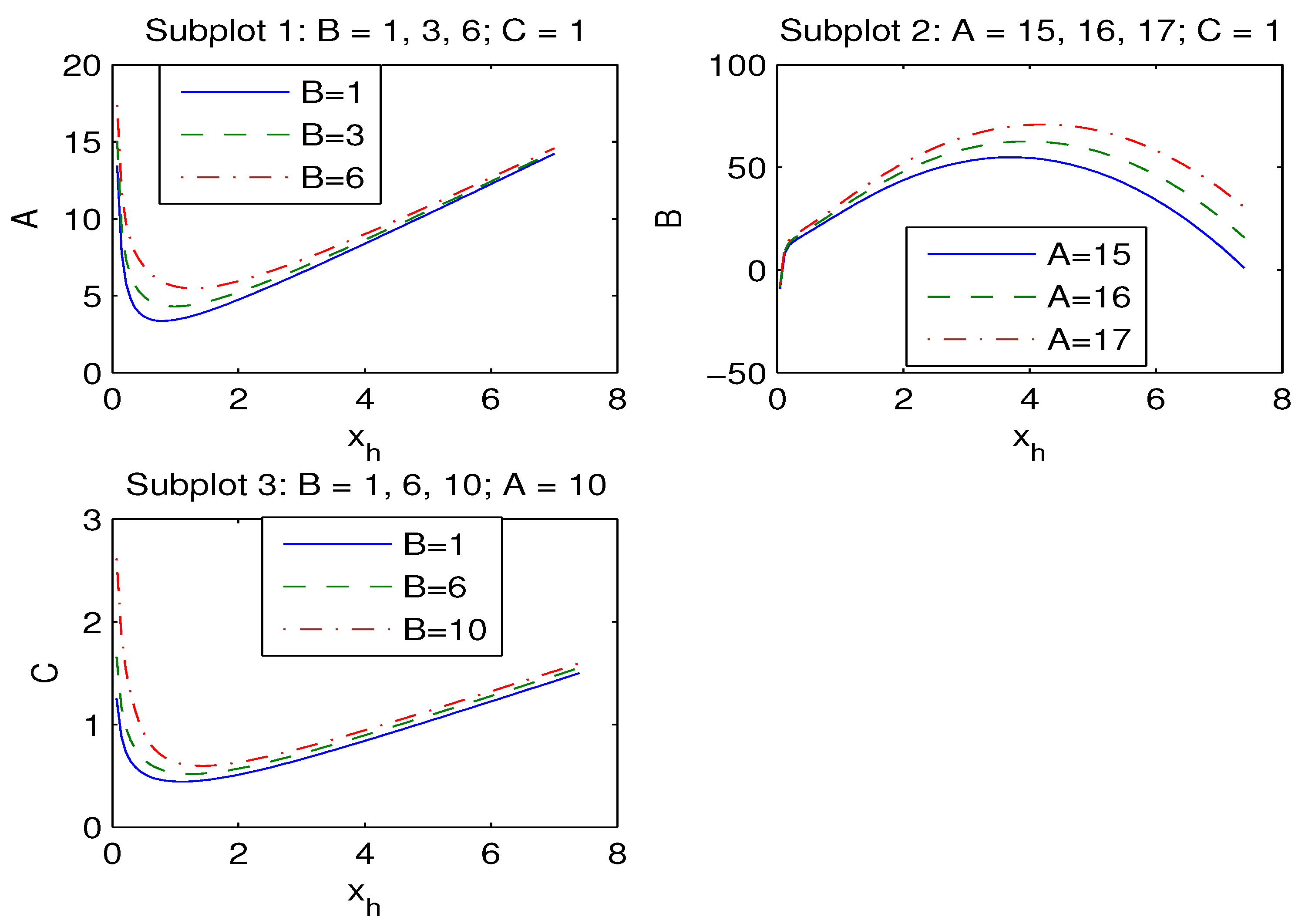
3. The BH Thermodynamics

Consider the BH thermodynamics and the thermal stability of the BH. The Hawking temperature is given by

$$T_H\left(r_{+}\right)=\frac{f^{\prime }\left(r\right){\mid }_{r=r_{+}}}{4\pi },$$

(15)

where $r_{+}$ is the event horizon radius defined by the biggest root of the equation $f\left(r_h\right)=0$. Making use of Equations (12) and (15), with the variable $x=2^{1/4}r/\sqrt[4]{\beta q^2}$, we obtain the Hawking temperature

$$T_H\left(x_{+}\right)=\frac{2^{1/4}}{4\pi \sqrt[4]{\beta q^2}}\left(\frac{2c{x}_{+}^2-1+B{C}^2{x}_{+}^2{g}^{\prime }\left(x_{+}\right)}{2x_{+}(1+c{x}_{+}^2)}\right),$$

(16)

$$g^{\prime }\left(x_{+}\right)=-\frac{1}{2x_{+}^2{cosh}^2(1/\left(2x_{+}\right))({tanh}^2(1/\left(2x_{+}\right))+1)},$$

where we substituted parameter A from equation $f\left(x_{+}\right)=0$. The plot of the dimensionless function $T_H\left(x_{+}\right)\sqrt[4]{\beta q^2}$ versus $x_{+}$ is depicted in Figure 2.

According to Figure 2, the Hawking temperature is positive in some range of $x_{+}$. To study the local stability of the BH, we calculate the heat capacity, making use of the expression

$$C_q\left(x_{+}\right)=T_H{\left(\frac{\partial S}{\partial T_H}\right)}_q=\frac{\partial M\left(x_{+}\right)}{\partial T_H\left(x_{+}\right)}=\frac{\partial M\left(x_{+}\right)/\partial x_{+}}{\partial T_H\left(x_{+}\right)/\partial x_{+}},$$

(17)

where $M\left(x_{+}\right)$ is the BH gravitational mass depending on the event horizon radius. From equation $f\left(x_{+}\right)=0$, one obtains the BH gravitational mass

$$M\left(x_{+}\right)=\frac{{\beta }^{3/4}{q}^{3/2}}{2^{15/4}\alpha G}\left(\frac{1+2C{x}_{+}^2}{C^2{x}_{+}}+Bg\left(x_{+}\right)\right).$$

(18)

With the aid of Equations (16) and (18), we find

$$\frac{\partial M\left(x_{+}\right)}{\partial x_{+}}=\frac{{\beta }^{3/4}{q}^{3/2}}{2^{15/4}\alpha G}\left(\frac{2C{x}_{+}^2-1}{C^2{x}_{+}^2}+B{g}^{\prime }\left(x_{+}\right)\right),$$

(19)

$$\frac{\partial T_H\left(x_{+}\right)}{\partial x_{+}}=\frac{1}{4\pi 2^{3/4}\sqrt[4]{\beta q^2}}(\frac{5C{x}_{+}^2-2C^2{x}_{+}^4+1}{x_{+}^2{(1+C{x}_{+}^2)}^2}$$

$$+\frac{B{C}^2[g^{\prime }\left(x_{+}\right)(1-C{x}_{+}^2)+x_{+}{g}^{″}\left(x_{+}\right)(1+C{x}_{+}^2)]}{{(1+C{x}_{+}^2)}^2}),$$

(20)

$$g^{″}\left(x_{+}\right)=\frac{({tanh}^2(1/\left(2x_{+}\right))+1)(2x_{+}-tanh(1/\left(2x_{+}\right)))}{2x_{+}^4{cosh}^2(1/\left(2x_{+}\right)){({tanh}^2(1/\left(2x_{+}\right))+1)}^2}$$

$$-\frac{tanh(1/\left(2x_{+}\right))}{2x_{+}^4{cosh}^4(1/\left(2x_{+}\right)){({tanh}^2(1/\left(2x_{+}\right))+1)}^2}.$$

According to Equation (17), the heat capacity possesses a singularity when the Hawking temperature has an extremum, $\partial T_H\left(x_{+}\right)/\partial x_{+}=0$. It follows from Equations (16) and (17) that at some point, $x_{+}=x_1$, the Hawking temperature and heat capacity are zero where a first-order phase transition occurs. In this point, $x_1$, the BH remnant with nonzero BH mass is formed, but the Hawking temperature and heat capacity become zero. In the point $x=x_2$, $\partial T_H\left(x_{+}\right)/\partial x_{+}=0$, the heat capacity has a discontinuity, and the second-order phase transition occurs. In the interval $x_2>x_{+}>x_1$, BHs are locally stable, and at $x_{+}>x_2$, the BH becomes unstable. By using Equations (17), (19) and (20), we represented the heat capacity in Figure 3.

In accordance with Figure 3, the BH is locally stable in the range $x_2>x_{+}>x_1$ with a positive Hawking temperature and heat capacity. The entropy S at the constant charge q could be calculated from the first law of BH thermodynamics $dM\left(x_{+}\right)=T_H\left(x_{+}\right)dS+\varphi dq$,

$$S=\int \frac{dM\left(x_{+}\right)}{T_H\left(x_{+}\right)}=\int \frac{1}{T_H\left(x_{+}\right)}\frac{\partial M\left(x_{+}\right)}{\partial x_{+}}d{x}_{+}.$$

(21)

It should be noted that the entropy in this expression is defined as a constant of integration. Making use of Equations (16), (19) and (21), we obtain the entropy

$$S=\frac{\pi \beta q^2}{8C^2\alpha G}\int \frac{1+C{x}_{+}^2}{x_{+}}d{x}_{+}=\frac{\pi r_{+}^2}{G}+\frac{4\pi \alpha }{G}ln\left(\frac{\sqrt[4]{2}{r}_{+}}{\sqrt[4]{\beta q^2}}\right)+ Constant,$$

(22)

where $Constant$ is the integration constant. One can see the discussion of integration constants in [50]. We choose the integration constant as

$$Constant=\frac{2\pi \alpha }{G}ln\left(\frac{\pi q\sqrt{\beta }}{\sqrt{2}G}\right).$$

(23)

From Equations (22) and (23), we find the BH entropy

$$S=S_0+\frac{2\pi \alpha }{G}ln\left(S_0\right),$$

(24)

where $S_0=\pi r_{+}^2/G$ is the Bekenstein–Hawking entropy. According to Equation (24), there is a logarithmic correction to area law. The entropy (24) does not contain the NED parameter $\beta$. The entropy (24) was obtained in 4D EGB gravity coupled with other NED models in [51,52,53]. Thus, entropy (24) does not depend on NED, which is due to the GB term in action, and the logarithmic correction vanishes when $\alpha =0$. At big $r_{+}$ (event horizon radii), the Bekenstein–Hawking entropy is dominant, and for small $r_{+}$, the logarithmic correction is important. It is worth noting that at some event horizon radius $r_0$, the entropy vanishes, and when $r_{+}<r_0$, the entropy becomes negative. The negative entropy of BHs was discussed in [7].

4. The Shadow of Black Holes

The shadow of the BH is due to the light gravitational lensing and is a black circular disk. The image of the super-massive M87* BH was observed by collaboration with the Event Horizon Telescope [48]. The shadow of a neutral Schwarzschild BH was investigated in [54]. The photons moving in the equatorial plane with $\vartheta =\pi /2$ will be considered. Making use of the Hamilton−Jacobi method, the photon motion in null curves is described by the Equation (see, for example, [55])

$$H=\frac{1}{2}{g}^{\mu \nu }{p}_{\mu }{p}_{\nu }=\frac{1}{2}\left(\frac{L^2}{r^2}-\frac{E^2}{f\left(r\right)}+\frac{{\dot{r}}^2}{f\left(r\right)}\right)=0,$$

(25)

where $p_{\mu }$ is the photon momentum, $\dot{r}=\partial H/\partial p_r$, and the energy and angular momentum of a photon, which are constants of motion, are defined by $E=-p_t$ and $L=p_{\varphi }$ . Equation (25) can be represented in the form

$$V+{\dot{r}}^2=0,V=f\left(r\right)\left(\frac{L^2}{r^2}-\frac{E^2}{f\left(r\right)}\right).$$

(26)

The radius of the photon circular orbit $r_p$ obeys the equation $V\left(r_p\right)=V^{\prime }{\left(r\right)}_{|r=r_p}=0$. From Equation (26), one obtains

$$\xi \equiv \frac{L}{E}=\frac{r_p}{\sqrt{f\left(r_p\right)}},f^{\prime }\left(r_p\right)r_p-2f\left(r_p\right)=0,$$

(27)

where $\xi$ is the impact parameter. The shadow radius $r_s$ for a distant observer, $r_0\to \infty$, reads $r_s=r_p/\sqrt{f\left(r_p\right)}$. Note that the impact parameter is $\xi =r_s$. The event horizon radius $r_{+}$ is the biggest root of the equation $f\left(r_h\right)=0$. Making use of Equation (12) and $f\left(r_h\right)=0$, one finds the parameters A, B and C versus $x_h$

$$A=\frac{1+2C{x}_h^2+C^2{x}_{h}Bg\left(x_h\right)}{C^2{x}_h},B=\frac{-1-2C{x}_h^2+C^2{x}_{h}A}{C^2{x}_{h}g\left(x_h\right)},$$

$$C=\frac{x_h^2+\sqrt{x_h^4+x_h(A-Bg\left(x_h\right))}}{x_h(A-Bg\left(x_h\right))},$$

(28)

where $x_h=r_h/\sqrt[4]{\beta q^2}$. The plots of functions (28) are given in Figure 4.

According to Figure 4 (Subplot 1), if parameter A increases, the event horizon radius $x_{+}$ also increases. Figure 4 (Subplot 2) shows that when parameter B increases, the event horizon radius decreases. According to Figure 4 (Subplot 3), if C increasing the event horizon radius $x_{+}$ also increasing.

In

Table 1. The event horizon, photon sphere and shadow dimensionless radii for $A=7$, $C=1$.

B	0.1	0.5	1	2	3	4	5	6
$x_{+}$	3.34	3.31	3.27	3.19	3.10	3.01	2.91	2.80
$x_p$	5.11	5.07	5.02	4.91	4.80	4.68	4.55	4.42
$x_s$	8.97	8.92	8.85	8.71	8.57	8.43	8.27	8.11

, we presents the photon sphere radii ($x_p$), the event horizon radii ($x_{+}$), and the shadow radii ($x_s$) for $A=7$ and $C=1$. The null geodesics radii $x_p$ belong to unstable orbits and correspond to the maximum of the potential $V\left(r\right)$ ($V^{″}\le 0$).

According to Table 1, when the parameter B increasing the shadow radius $x_s$ decreases. Because $x_s>x_{+}$, the BH shadow radius is given by the radius $r_s=x_s\sqrt[4]{\beta q^2}/2^{1/4}$.

It is worth noting that nonlinear interaction of fields in the framework of NED leads to self-interaction, and photons propagate along null geodesics of the effective metric [56,57]. However, corrections in radii of photon spheres and impact parameters (due to the self-interaction of electromagnetic fields) are small [58].

5. The Energy Emission Rate of Black Holes

For the observer at infinity, the BH shadow is linked with the high energy absorption cross section [43,59]. The absorption cross section, at very high energies, oscillates around the photon sphere $\sigma \approx \pi r_s^2$, and the BH energy emission rate is expressed as

$$\frac{d^{2}E\left(\omega \right)}{dtd\omega }=\frac{2{\pi }^3{\omega }^3{r}_s^2}{exp\left(\omega /T_H\left(r_{+}\right)\right)-1},$$

(29)

where $\omega$ is the emission frequency. From Equations (16) and (29), we obtain the BH energy emission rate in terms of the dimensionless variable $x_{+}=2^{1/4}{r}_{+}/\sqrt[4]{\beta q^2}$

$${\beta }^{1/4}\sqrt{q}\frac{d^{2}E\left(\omega \right)}{dtd\omega }=\frac{2{\pi }^3{\varpi }^3{x}_s^2}{exp\left(\varpi /{\overline{T}}_H\left(x_{+}\right)\right)-1},$$

(30)

where ${\overline{T}}_H\left(x_{+}\right)={\beta }^{1/4}\sqrt{q}{T}_H\left(x_{+}\right)$, and $\varpi ={\beta }^{1/4}\sqrt{q}\omega$. The radiation rate, as a function of the dimensionless emission frequency $\overline{\omega }$ for $C=1$, $A=7$ and $B=0.1,3,6$, is plotted in Figure 5.

According to Figure 5, we have a peak of the BH energy emission rate. If the parameter B increases, the peak of the energy emission rate becomes smaller and is in the low frequency. At a bigger parameter B, the BH possesses a bigger lifetime.

6. Quasinormal Modes

Information about the stability of BHs under small perturbations can be obtained by studying quasinormal modes (QNMs), which are characterized by complex frequencies $\omega$. The mode is stable when Im $\omega <0$ otherwise it is unstable. In the eikonal limit Re, $\omega$ is connected with the radius of the BH shadow [60,61]. The perturbations by a scalar massless field around BHs are described by the effective potential barrier

$$V\left(r\right)=f\left(r\right)\left(\frac{f^{\prime }\left(r\right)}{r}+\frac{l(l+1)}{r^2}\right),$$

(31)

where l is the multipole number $l=0,1,2\dots$. Equation (27) can be represented as

$$V\left(x\right)\sqrt{\beta }q=\sqrt{2}f\left(x\right)\left(\frac{f^{\prime }\left(x\right)}{x}+\frac{l(l+1)}{x^2}\right).$$

(32)

The dimensionless potential $V\left(x\right)\sqrt{\beta }q$ is given in Figure 6 for $A=7$, $B=1$, $C=1$ (Subplot 1), and $l=3,4,5$ and for $A=7$, $C=1$, $l=5$, and $B=1,3,6$ (Subplot 2).

Figure 6, Subplot l, shows that the potential barriers of effective potentials have the maxima. When the l increases, the height of the potential increases. According to Figure 6, Subplot 2, if the parameter B increases, the height of the potential increases. The quasinormal frequencies can be found by [60,61]

$$\mathrm{Re}\omega =\frac{l}{r_s}=\frac{l\sqrt{f\left(r_p\right)}}{r_p},\mathrm{Im}\omega =-\frac{2n+1}{2\sqrt{2}{r}_s}\sqrt{2f\left(r_p\right)-r_p^2{f}^{″}\left(r_p\right)},$$

(33)

where $r_s$ is the BH shadow radius, $r_p$ is the BH photon sphere radius, and $n=0,1,2,\dots$ is the overtone number. The frequencies, depending on parameter B (at $A=7$, $C=1$, $n=1$, $l=5$), are represented in

Table 2. The real and the imaginary parts of the frequencies vs. the parameter B at $n=1$, $l=5$, $A=7$, $C=1$.

B	0.1	0.5	1	2	3	4	5	6
$\sqrt[4]{\beta q^2}\mathrm{Re}\omega$	0.557	0.561	0.565	0.574	0.583	0.593	0.605	0.617
$-\sqrt[4]{\beta q^2}\mathrm{Im}\omega$	0.3212	0.3215	0.3221	0.3229	0.3234	0.3232	0.3230	0.3220

.

The modes are stable (the real part represents the frequency of oscillations) because the imaginary parts of the frequencies in Table 2 are negative. Table 2 shows that when parameter B increases the real part of the frequency $\sqrt[4]{\beta q^2}\mathrm{Re},\omega$ increases, and the absolute value of the imaginary part of the frequency $\mid \sqrt[4]{\beta q^2}\mathrm{Im}\omega \mid$ increases. Therefore, when parameter B is increased, the scalar perturbations oscillate with greater frequency and decay fast.

7. Conclusions

We obtained the exact spherically symmetric and magnetized BH solution in 4D EGB gravity coupled with NED. The thermodynamics and the thermal stability of magnetically charged BHs were studied by calculating the Hawking temperature and the heat capacity. The phase transitions occur in the points where the Hawking temperature possesses the extremum. It is shown that BHs are thermodynamically stable at some interval of event horizon radii when the heat capacity and the Hawking temperature are positive. The heat capacity possesses a singularity in some event horizon radii where the second-order phase transitions occur. The entropy of BHs is calculated, including the Hawking entropy and the logarithmic correction. The photon sphere radii, the event horizon radii, and the shadow radii are calculated. We show that with increasing the model parameter B, the BH energy emission rate decreases and, as a result, the BH has a longer lifetime. The quasinormal modes are investigated and it is shown that increasing the parameter B the scalar perturbations oscillate with greater frequency and decay fast. It is worth noting that other solutions in 4D EGB gravity coupled with some NED were obtained in [51,52,53]. It is of interest to study solutions of BHs in 4D EGB gravity coupled with different NED because astrophysical characteristics depend on them.

References

1. Gross, D.J.; Witten, E. Superstring modifications of Einstein’s equations. Nucl. Phys. B 1986, 277, 1–10. [Google Scholar] [CrossRef]
2. Gross, D.J.; Sloan, J.H. The quartic effective action for the heterotic string. Nucl. Phys. B 1987, 291, 41–89. [Google Scholar] [CrossRef]
3. Metsaev, R.R.; Tseytlin, A.A. Two-loop β-function for the generalized bosonic sigma model. Phys. Lett. B 1987, 191, 354–362. [Google Scholar] [CrossRef]
4. Zwiebach, B. Curvature squared terms and string theories. Phys. Lett. B 1985, 156, 315–317. [Google Scholar] [CrossRef]
5. Metsaev, R.R.; Tseytlin, A.A. Order α (two-loop) equivalence of the string equations of motion and the σ-model Weyl invariance conditions: Dependence on the dilaton and the antisymmetric tensor. Nucl. Phys. B 1987, 293, 385–419. [Google Scholar] [CrossRef]
6. Glavan, D.; Lin, C. Einstein–Gauss–Bonnet gravity in four-dimensional spacetime. Phys. Rev. Lett. 2020, 124, 081301. [Google Scholar] [CrossRef] [PubMed] [Green Version]
7. Cvetic, M.; Nojiri, S.I.; Odintsov, S.D. Black hole thermodynamics and negative entropy in de Sitter and anti-de Sitter Einstein–Gauss–Bonnet gravity. Nucl. Phys. B 2002, 628, 295–330. [Google Scholar] [CrossRef] [Green Version]
8. Boulware, D.G.; Deser, S. String-generated gravity models. Phys. Rev. Lett. 1985, 55, 2656–2660. [Google Scholar] [CrossRef] [Green Version]
9. Wheeler, J.T. Symmetric solutions to the Gauss–Bonnet extended Einstein equations. Nucl. Phys. B 1986, 268, 737–746. [Google Scholar] [CrossRef]
10. Myers, R.C.; Simon, J.Z. Black-hole thermodynamics in Lovelock gravity. Phys. Rev. D 1988, 38, 2434–2444. [Google Scholar] [CrossRef] [Green Version]
11. Lovelock, D.J. The Einstein tensor and its generalizations. Math. Phys. 1971, 12, 498–501. [Google Scholar] [CrossRef]
12. Cai, R.G.; Cao, L.M.; Ohta, N. Black holes in gravity with conformal anomaly and logarithmic term in black hole entropy. J. High Energy Phys. 2010, 1004, 82. [Google Scholar] [CrossRef] [Green Version]
13. Cai, R.-G. Thermodynamics of conformal anomaly corrected black holes in AdS space. Phys. Lett. B 2014, 733, 183–189. [Google Scholar] [CrossRef] [Green Version]
14. Cognola, G.; Myrzakulov, R.; Sebastiani, L.; Zerbini, S. Einstein gravity with Gauss-Bonnet entropic corrections. Phys. Rev. D 2013, 88, 024006. [Google Scholar] [CrossRef] [Green Version]
15. Fernandes, P.G.S. Charged black holes in AdS spaces in 4D Einstein Gauss–Bonnet gravity. Phys. Lett. B 2020, 805, 135468. [Google Scholar] [CrossRef]
16. Jusufi, K. Nonlinear magnetically charged black holes in 4D Einstein–Gauss–Bonnet gravity. Ann. Phys. 2020, 421, 168285. [Google Scholar] [CrossRef]
17. Ghosh, S.G.; Singh, D.V.; Kumar, R.; Maharaj, S.D. Phase transition of AdS black holes in 4D EGB gravity coupled to nonlinear electrodynamics. Ann. Phys. 2021, 424, 168347. [Google Scholar] [CrossRef]
18. Ghosh, S.G.; Maharaj, S.D. Radiating black holes in the novel 4D Einstein–Gauss–Bonnet gravity. Phys. Dark Univ. 2020, 30, 100687. [Google Scholar] [CrossRef]
19. Kumar, R.; Ghosh, S.G. Rotating black holes in 4D Einstein–Gauss–Bonnet gravity and its shadow. J. Cosmol. Astro. Phys 2020, 7, 53. [Google Scholar] [CrossRef]
20. Jin, X.H.; Gao, Y.X.; Liu, D.J. Strong gravitational lensing of a 4D Einstein–Gauss–Bonnet black hole in homogeneous plasma. Int. J. Mod. Phys. D 2020, 29, 2050065. [Google Scholar] [CrossRef]
21. Jusufi, K.; Banerjee, A.; Ghosh, S.G. Wormholes in 4D Einstein–Gauss–Bonnet gravity. Eur. Phys. J. C 2020, 80, 698. [Google Scholar] [CrossRef]
22. Guo, M.; Li, P. Innermost stable circular orbit and shadow of the 4D Einstein–Gauss–Bonnet black hole. Eur. Phys. J. C 2020, 80, 588. [Google Scholar] [CrossRef]
23. Zhang, C.; Zhang, S.; Li, P.; Guo, M. Superradiance and stability of the regularized 4D charged Einstein–Gauss–Bonnet black hole. J. High Energy Phys. 2020, 8, 105. [Google Scholar] [CrossRef]
24. Odintsov, S.; Oikonomou, V.; Fronimos, F. Rectifying Einstein–Gauss–Bonnet inflation in view of GW170817. Nucl. Phys. B 2020, 958, 115135. [Google Scholar] [CrossRef]
25. Ai, W. A note on the novel 4D Einstein–Gauss–Bonnet gravity. Commun. Theor. Phys. 2020, 72, 095402. [Google Scholar] [CrossRef]
26. Fernandes, P.G.; Carrilho, P.; Clifton, T.; Mulryne, D.J. Derivation of regularized field equations for the Einstein–Gauss–Bonnet theory in four dimensions. Phys. Rev. D 2020, 102, 024025. [Google Scholar] [CrossRef]
27. Hennigar, R.A.; Kubiznak, D.; Mann, R.B.; Pollack, C. On taking the D→4 limit of Gauss–Bonnet gravity: Theory and solutions. J. High Energy Phys. 2020, 2020, 27. [Google Scholar] [CrossRef]
28. Gurses, M.; Sisman, T.C.; Tekin, B. Comment on “Einstein–Gauss–Bonnet Gravity in 4-Dimensional Space-Time”. Phys. Rev. Lett. 2020, 125, 149001. [Google Scholar] [CrossRef]
29. Gurses, M.; Sisman, T.C.; Tekin, B. Is there a novel Einstein–Gauss–Bonnet theory in four dimensions? Eur. Phys. J. C 2020, 80, 647. [Google Scholar] [CrossRef]
30. Mahapatra, S. A note on the total action of 4D Gauss–Bonnet theory. Eur. Phys. J. C 2020, 80, 992. [Google Scholar] [CrossRef]
31. Arrechea, J.; Delhom, A.; Jiménez-Cano, A. Inconsistencies in four-dimensional Einstein–Gauss–Bonnet gravity gravity. Chin. Phys. C 2021, 45, 013107. [Google Scholar] [CrossRef]
32. Arrechea, J.; Delhom, A.; Jiménez-Cano, A. Comment on “Einstein–Gauss–Bonnet Gravity in Four-Dimensional Spacetime”. Phys. Rev. Lett. 2020, 125, 149002. [Google Scholar] [CrossRef]
33. Hohmann, M.; Pfeifer, C. Canonical variational completion and 4D Einstein–Gauss–Bonnet gravity. Eur. Phys. J. Plus 2021, 136, 180. [Google Scholar] [CrossRef]
34. Kobayashi, T. Effective scalar-tensor description of regularized Lovelock gravity in four dimensions. J. Cosmol. Astro. Phys. 2020, 7, 13. [Google Scholar] [CrossRef]
35. Bonifacio, J.; Hinterbichler, K.; Johnson, L.A. Amplitudes and 4D Gauss–Bonnet Theory. Phys. Rev. D 2020, 102, 024029. [Google Scholar] [CrossRef]
36. Aoki, K.; Gorji, M.A.; Mukohyama, S. A consistent theory of D→4 Einstein-Gauss-Bonnet gravity. Phys. Lett. B 2020, 810, 135843. [Google Scholar] [CrossRef]
37. Aoki, K.; Gorji, M.A.; Mukohyama, S. A consistent theory of D→4 Einstein–Gauss–Bonnet gravity. J. Cosmol. Astro. Phys. 2020, 2009, 14. [Google Scholar] [CrossRef]
38. Aoki, K.; Gorji, M.A.; Mizuno, S.; Mukohyama, S. Cosmology and gravitational waves in consistent D→4 Einstein–Gauss–Bonnet gravity. J. Cosmol. Astro. Phys. 2021, 2101, 54. [Google Scholar] [CrossRef]
39. Jafarzade, K.; Zangeneh, M.K.; Lobo, F.S.N. Shadow, deflection angle and quasinormal modes of Born-Infeld charged black holes. J. Cosmol. Astro. Phys. 2021, 4, 8. [Google Scholar] [CrossRef]
40. Kruglov, S.I. Magnetically charged black hole in frameworkof nonlinear electrodynamics model. Int. J. Mod. Phys. A 2018, 33, 1850023. [Google Scholar] [CrossRef]
41. Konoplya, R.A.; Zinhailo, A.F. Quasinormal modes, stability and shadows of a black hole in the 4D Einstein–Gauss–Bonnet gravity. Eur. Phys. J. C 2020, 80, 1049. [Google Scholar] [CrossRef]
42. Konoplya, R.A.; Zinhailo, A.F. 4D Einstein–Lovelock black holes: Hierarchy of orders in curvature. Phys. Lett. B 2020, 807, 135607. [Google Scholar] [CrossRef]
43. Belhaj, A.; Benali, M.; Balali, A.E.; Moumni, H.E.; Ennadifi, S.E. Deflection Angle and Shadow Behaviors of Quintessential Black Holes in arbitrary Dimensions. Class. Quant. Grav. 2020, 37, 215004. [Google Scholar] [CrossRef]
44. Konoplya, R.A.; Stuchlik, Z. Are eikonal quasinormal modes linked to the unstable circular null geodesics? Phys. Lett. B 2017, 771, 597. [Google Scholar] [CrossRef]
45. Stefanov, I.Z.; Yazadjiev, S.S.; Gyulchev, G.G. Connection between black-hole quasinormal modes and lensing in the strong deflection limit. Phys. Rev. Lett. 2010, 104, 251103. [Google Scholar] [CrossRef] [Green Version]
46. Guo, Y.; Miao, Y.G. Null geodesics, quasinormal modes and the correspondence with shadows in high-dimensional Einstein–Yang–Mills spacetimes. Phys. Rev. D 2020, 102, 084057. [Google Scholar] [CrossRef]
47. Wei, S.W.; Liu, Y.X. Null geodesics, quasinormal modes, and thermodynamic phase transition for charged black holes in asymptotically flat and dS spacetimes. Chin. Phys. C 2020, 44, 115103. [Google Scholar] [CrossRef]
48. Event Horizon Telescope Collaboration; Akiyama, K. First M87 event horizon telescope results. V. Physical origin of the asymmetric ring. Astrophys. J. 2019, 875, L5. [Google Scholar]
49. Dokuchaev, V.I.; Nazarova, N.O. Silhouettes of invisible black holes. Usp. Fiz. Nauk 2020, 190, 627. [Google Scholar] [CrossRef] [Green Version]
50. Medved, A.J.M.; Vagenas, E.C. When conceptual worlds collide: The GUP and the BH entropy. Phys. Rev. D 2004, 70, 124021. [Google Scholar] [CrossRef] [Green Version]
51. Kruglov, S.I. Einstein–Gauss–Bonnet gravity with nonlinear electrodynamics. Ann. Phys. 2021, 428, 168449. [Google Scholar] [CrossRef]
52. Kruglov, S.I. Einstein–Gauss–Bonnet Gravity with Nonlinear Electrodynamics: Entropy, Energy Emission, Quasinormal Modes and Deflection Angle. Symmetry 2021, 13, 944. [Google Scholar] [CrossRef]
53. Kruglov, S.I. Einstein–Gauss–Bonnet gravity with rational nonlinear electrodynamics. EPL 2021, 133, 69001. [Google Scholar] [CrossRef]
54. Synge, J.L. The escape of photons from gravitationally intense stars. Mon. Not. Roy. Astron. Soc. 1966, 131, 463. [Google Scholar] [CrossRef]
55. Kruglov, S.I. 4D Einstein–Gauss–Bonnet Gravity Coupled with Nonlinear Electrodynamics. Symmetry 2021, 13, 204. [Google Scholar] [CrossRef]
56. Novello, M.; Lorenci, V.A.D.; Salim, J.M.; Klippert, R. Geometrical aspects of light propagation in nonlinear electrodynamics. Phys. Rev. D 2000, 61, 045001. [Google Scholar] [CrossRef] [Green Version]
57. Novello, M.; Bergliaffa, S.E.P.; Salim, J.M. Singularities in general relativity coupled to nonlinear electrodynamics. Class. Quant. Grav. 2000, 17, 3821. [Google Scholar] [CrossRef] [Green Version]
58. Kocherlakota, P.; Rezzolla, L. Accurate mapping of spherically symmetric black holes in a parametrized framework. Phys. Rev. D 2020, 6, 064058. [Google Scholar] [CrossRef]
59. Wei, S.W.; Liu, Y.X. Observing the shadow of Einstein–Maxwell-Dilaton-Axion black hole. J. Cosmol. Astropart. Phys. 2013, 11, 63. [Google Scholar] [CrossRef] [Green Version]
60. Jusufi, K. Quasinormal Modes of Black Holes Surrounded by Dark Matter and Their Connection with the Shadow Radius. Phys. Rev. D 2020, 101, 084055. [Google Scholar] [CrossRef] [Green Version]
61. Jusufi, K. Connection Between the Shadow Radius and Quasinormal Modes in Rotating Spacetimes. Phys. Rev. D 2020, 101, 124063. [Google Scholar] [CrossRef]
Figure 1. The plot of the function f ( x ) for A = 7 , C = 1 .
Universe 07 00249 g001
Figure 2. The plot of the function T H ( x + ) β q 2 4 at C = 1 .
Universe 07 00249 g002
Figure 3. The plot of the function C q ( x + ) α G / ( β q 2 ) at C = 1 .
Universe 07 00249 g003
Figure 4. The plot of the functions A(xh), B(xh), C(xh). (A): Subplot 1: B = 1, 3, 6; C = 1; (B): Subplot 2: A = 15, 16, 17; C = 1; (C): Subplot 3: B = 1, 6, 10; A = 10.
Universe 07 00249 g004
Figure 5. The plot of the function β 1 / 4 q d 2 E ( ω ) d t d ω vs. ϖ for B = 0.1 , 3 , 6 , A = 7 , C = 1 .
Universe 07 00249 g005
Figure 6. The plot of the function V ( x ) β q for A = 7 , C = 1 .
Universe 07 00249 g006