
Next Generation Design and Prospects for Cannex


Abstract
:1. Introduction
2. Overview Dark Sector Interactions
2.1. Dark Matter
2.2. Dark Energy
3. The Quantum Vacuum and the Casimir Effect
4. Force Metrology with Macroscopic Objects
5. New Design
5.1. Core Setup and Measurement Principle
5.2. Parallelism
5.3. Surface Flatness
- Stochastic short-scale roughness with RMS amplitude . In this limit, the actual height distribution function can be used to statistically evaluate Equation (25). While, for an actual experiment, the statistics of measured surface profiles have to be evaluated, we choose here a normal distribution around zero . The error then results fromand is the peak roughness amplitude assumed to be equal on both plates.
- Large-scale deformations of the plates. For the lower plate of the recent experiment [49], the surface was measured using an optical profilometer to have a roughly spherical deformation of depth 15 nm (peak-peak) in negative direction (sag). It is technically, possible to obtain less than 10 nm sag, and the actual deformations can be measured with < nm accuracy. For the upper plate, we estimate the bend-through under gravity for a simply supported circular shell using the expression [207]Here, kg is the mass of the upper plate, , mm is the plate radius, μm is the plate thickness, and we use the values GPa and for the Young’s modulus and Poisson ratio, respectively, of silicon along the axis [205]. Equation (27) yields nm maximum bend-through at the center (). The error is then computed using Equation (25).
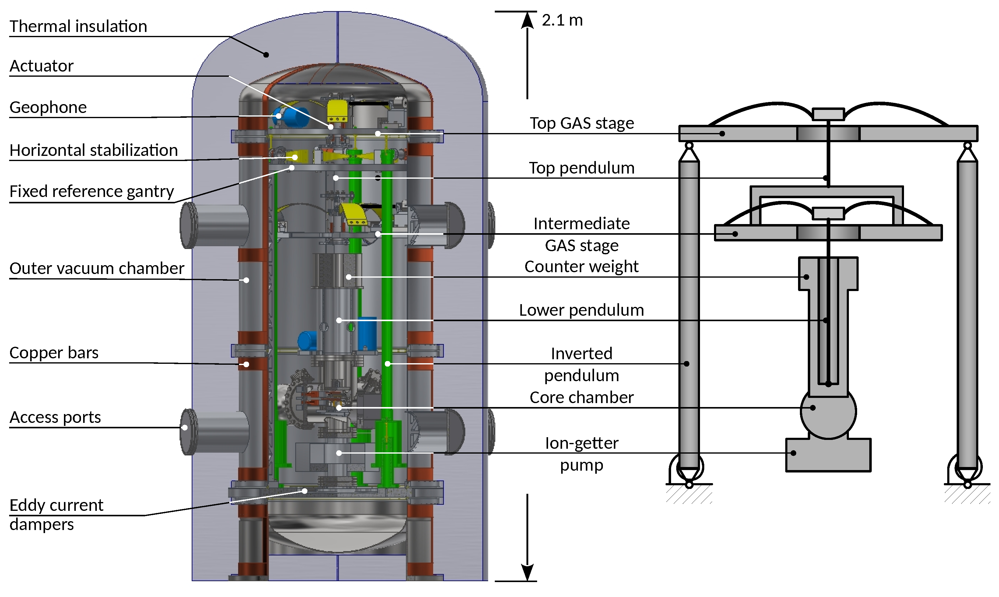
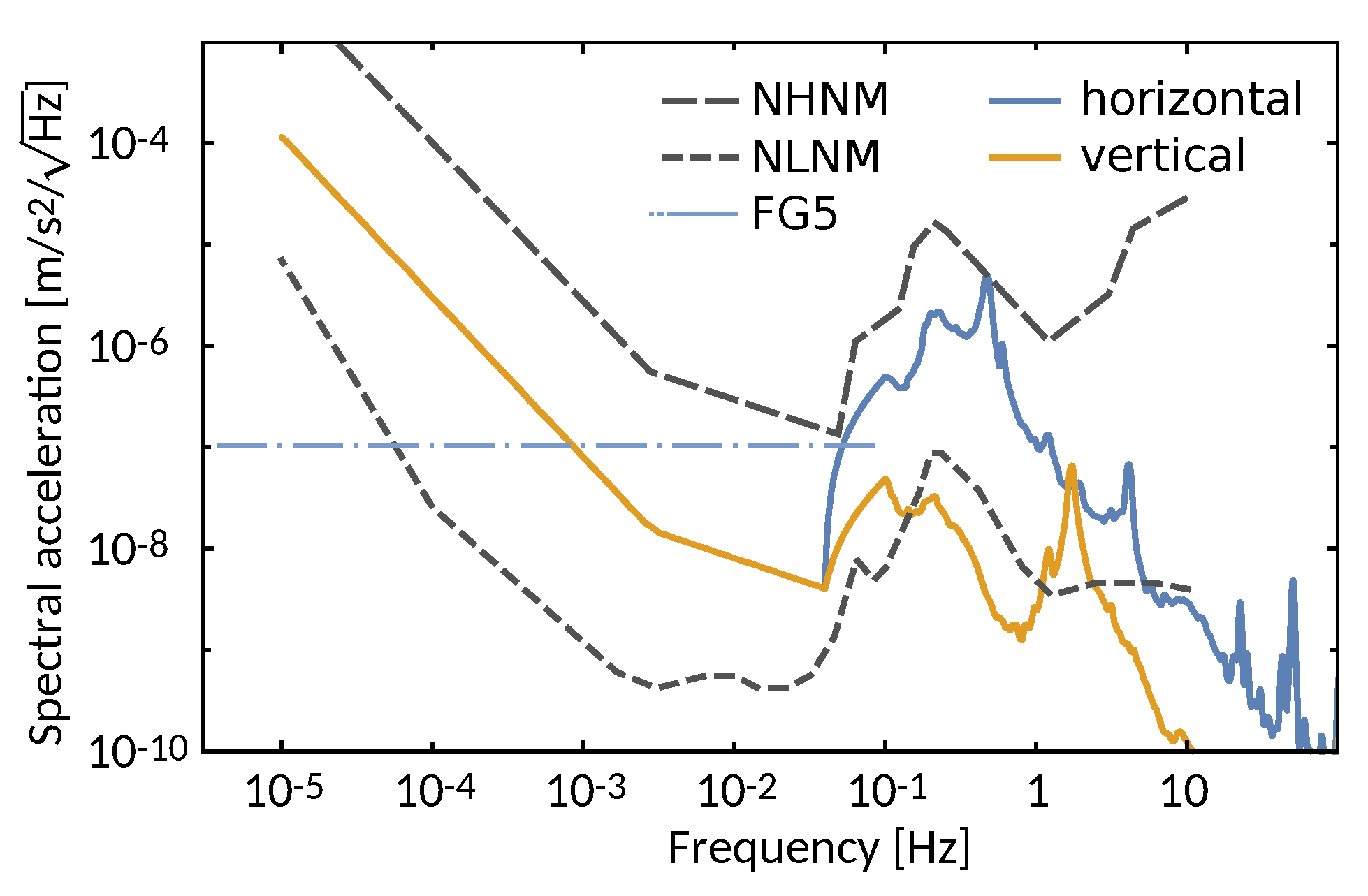
5.4. Vibrations and Seismic Isolation System
5.5. Thermal Errors and Control
5.6. Electrostatic Patch Effects
5.7. Detection Errors
5.8. Total Realistic Error Estimate
6. Prospects
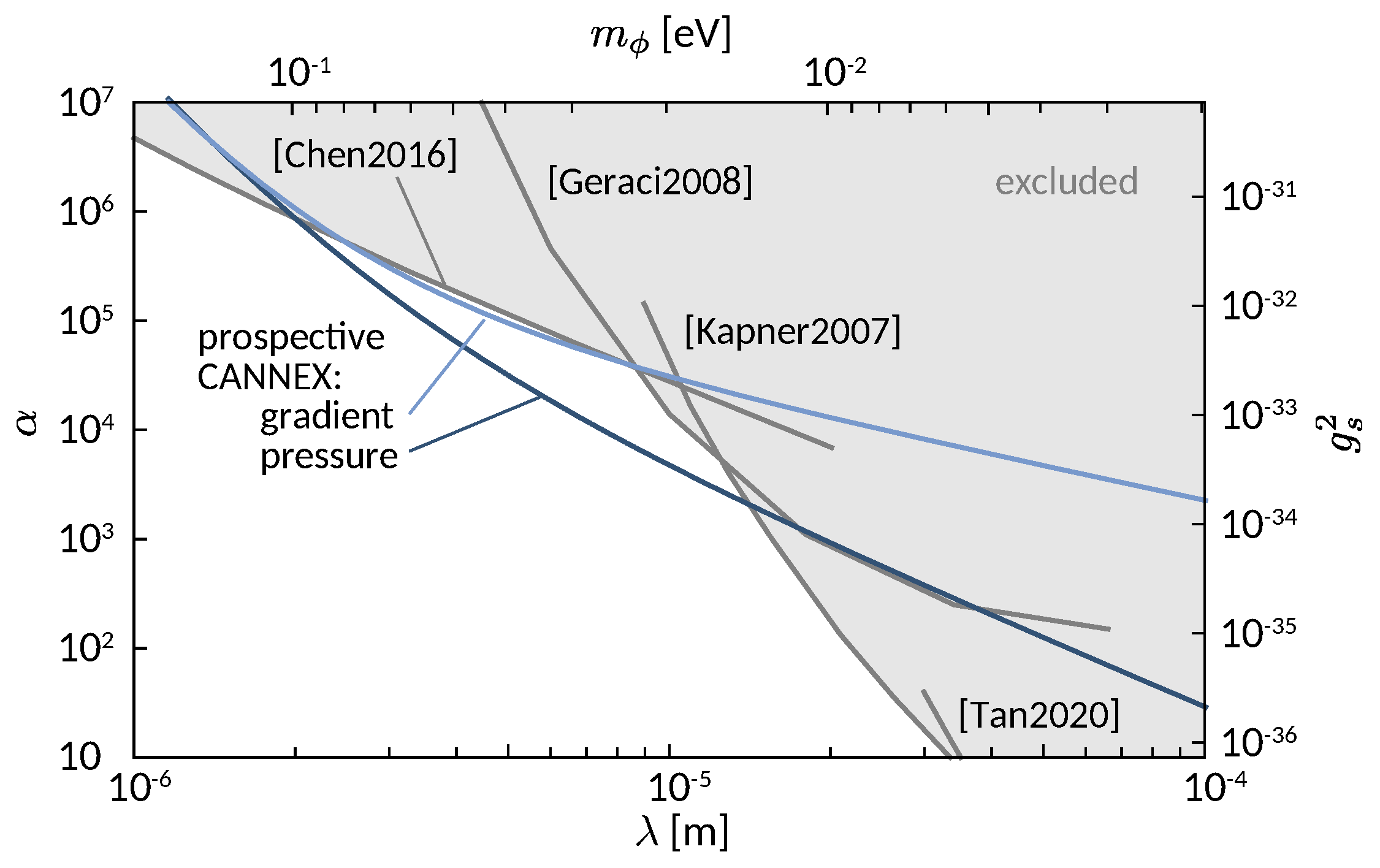
6.1. Casimir Interactions
6.2. Dark Matter
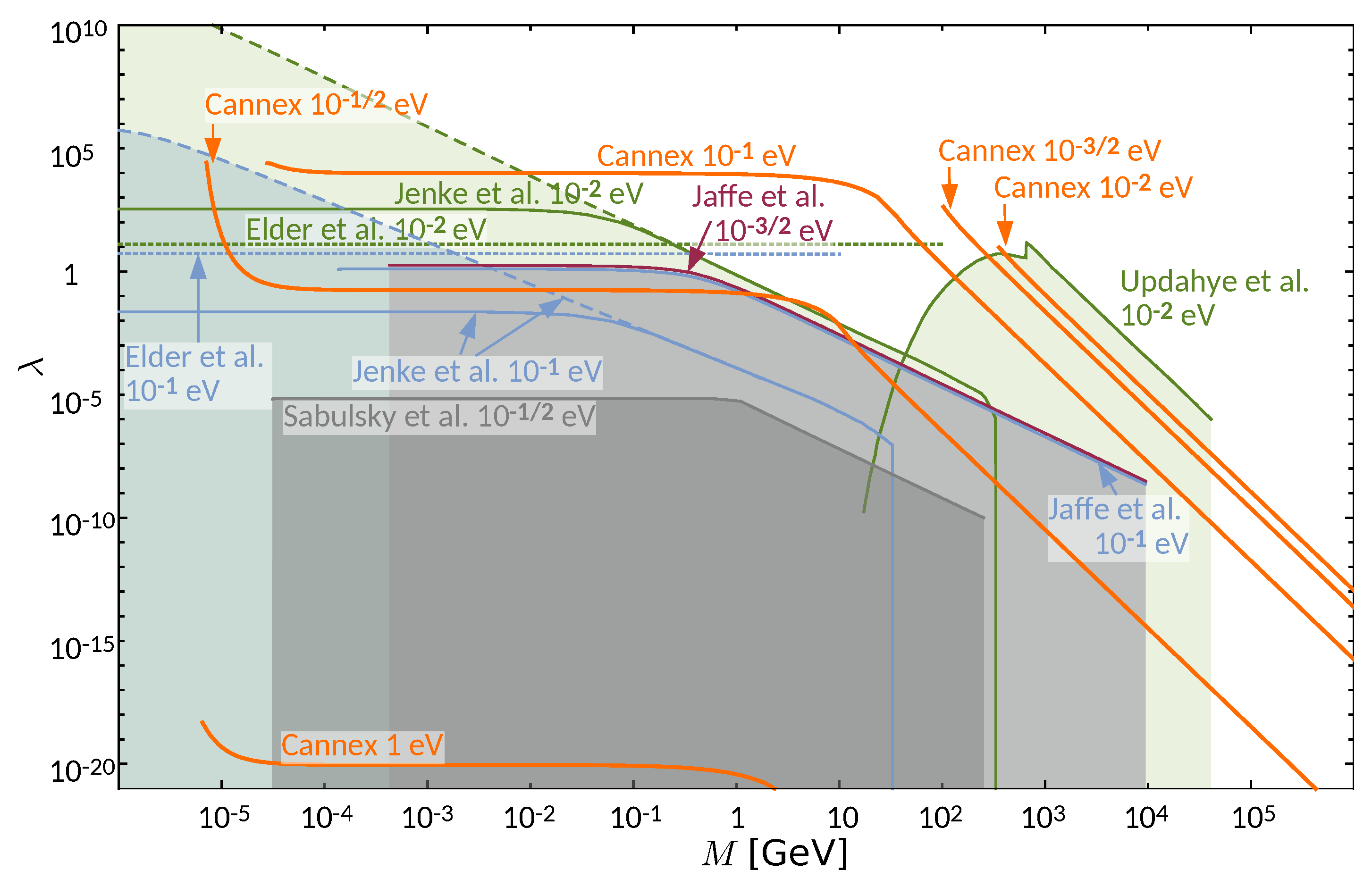
6.3. Dark Energy
7. Conclusions
Author Contributions
Funding
Institutional Review Board Statement
Informed Consent Statement
Data Availability Statement
Acknowledgments
Conflicts of Interest
Appendix A. Errors Due to Vibration


| 1 | |
| 2 | It must be noted that similar results, though mostly ignored by the Casimir community, have been obtained earlier in colloidal science, with respect to the van der Waals force being a manifestation of the same quantum effects that give rise to Casimir forces. |
| 3 | The real and imaginary parts of the complex dielectric susceptibilities are usually denoted as with a similar notation for the complex magnetic susceptibilities. |
| 4 | The appearance of complex functions results from the infinite integration of the mode density functions over real frequencies. As the latter have poles, the integration contour splits into a half-circle at infinity and an integration from to + . The former term vanishes due to for , leaving the integration over the complex frequency axis. |
| 5 | Note that, for graphene, the thermal contribution to the Casimir effect is significant at much smaller separations [178]. However, this effect could not be measured yet. |
| 6 | Note that the actual quantity measured in torsion pendula experiments is a torque. For the purpose of comparing the order-of-magnitude sensitivity of Ref. [32] to other experiments with force detection, we divide the torque sensitivity fNm by the effective radius of the test mass. For comparing the pressure (again only as rough estimation), we assume the entire torque-generating area of 10 2 to contribute homogeneously. |
| 7 | This form of connection is similar to a jewel bearing. Further contact is made via the three glass fibers having low thermal conductance ∼ W/m K [217] and three thin wires establishing electrical contact that, however, are thermalized via the Peltier element. |
| 8 | Here, we preclude that any hypothetical force will be much smaller than the Casimir force, as the latter has been measured at the percent level without significant disturbance. However, we may not a priori exclude the possibility that a hypothetical additional force may be responsible for the discrepancy between data and predictions by Lifshitz theory with the Drude model discussed in Section 6.1. |
| 9 | Note that, due to time constraints during manuscript preparation, we show in Figure 10 only and calculated using the Drude model, rather than the plasma model. |
References
- Bull, P.; Akrami, Y.; Adamek, J.; Baker, T.; Bellini, E.; Beltrán Jiménez, J.; Bentivegna, E.; Camera, S.; Clesse, S.; Davis, J.H.; et al. Beyond ΛCDM: Problems, Solutions, and the Road Ahead. Phys. Dark Univ. 2016, 12, 56–99. [Google Scholar] [CrossRef] [Green Version]
- Ade, P.A.R.; Aghanim, N.; Arnaud, M.; Ashdown, M.; Aumont, J.; Baccigalupi, C.; Banday, A.J.; Barreiro, R.B.; Bartlett, J.G.; Bartolo, N.; et al. Planck 2015 Results. XIII. Cosmological Parameters. Astron. Astrophys. 2016, 594, A13. [Google Scholar] [CrossRef] [Green Version]
- Aghanim, N.; Akrami, Y.; Ashdown, M.; Aumont, J.; Baccigalupi, C.; Ballardini, M.; Banday, A.J.; Barreiro, R.B.; Bartolo, N.; Basak, S.; et al. Planck 2018 Results. VI. Cosmological Parameters. Astron. Astrophys. 2020, 641, A6. [Google Scholar] [CrossRef] [Green Version]
- Raveri, M.; Hu, W. Concordance and Discordance in Cosmology. Phys. Rev. D 2019, 99, 043506. [Google Scholar] [CrossRef] [Green Version]
- Riess, A.G.; Casertano, S.; Yuan, W.; Macri, L.M.; Scolnic, D. Large Magellanic Cloud Cepheid Standards Provide a 1% Foundation for the Determination of the Hubble Constant and Stronger Evidence for Physics beyond ΛCDM. Astrophys. J. 2019, 876, 85. [Google Scholar] [CrossRef]
- Jee, I.; Suyu, S.H.; Komatsu, E.; Fassnacht, C.D.; Hilbert, S.; Koopmans, L.V.E. A Measurement of the Hubble Constant from Angular Diameter Distances to Two Gravitational Lenses. Science 2019, 365, 1134–1138. [Google Scholar] [CrossRef] [PubMed] [Green Version]
- Di Valentino, E.; Melchiorri, A.; Silk, J. Planck Evidence for a Closed Universe and a Possible Crisis for Cosmology. Nat. Astron. 2020, 4, 196–203. [Google Scholar] [CrossRef] [Green Version]
- Battye, R.A.; Charnock, T.; Moss, A. Tension between the Power Spectrum of Density Perturbations Measured on Large and Small Scales. Phys. Rev. D 2015, 91, 103508. [Google Scholar] [CrossRef] [Green Version]
- Abbott, T.M.C.; Abdalla, F.B.; Alarcon, A.; Aleksić, J.; Allam, S.; Allen, S.; Amara, A.; Annis, J.; Asorey, J.; Avila, S.; et al. Dark Energy Survey Year 1 Results: Cosmological Constraints from Galaxy Clustering and Weak Lensing. Phys. Rev. D 2018, 98, 043526. [Google Scholar] [CrossRef] [Green Version]
- Haslbauer, M.; Banik, I.; Kroupa, P.; Grishunin, K. The Ultra-Diffuse Dwarf Galaxies NGC 1052-DF2 and 1052-DF4 Are in Conflict with Standard Cosmology. Mon. Not. R. Astron. Soc. 2019, 489, 2634–2651. [Google Scholar] [CrossRef] [Green Version]
- Aguilar-Arevalo, A.A.; Brown, B.C.; Bugel, L.; Cheng, G.; Conrad, J.M.; Cooper, R.L.; Dharmapalan, R.; Diaz, A.; Djurcic, Z.; Finley, D.A.; et al. Significant Excess of Electronlike Events in the MiniBooNE Short-Baseline Neutrino Experiment. Phys. Rev. Lett. 2018, 121, 221801. [Google Scholar] [CrossRef] [Green Version]
- Aguilar, A.; Auerbach, L.B.; Burman, R.L.; Caldwell, D.O.; Church, E.D.; Cochran, A.K.; Donahue, J.B.; Fazely, A.; Garvey, G.T.; Gunasingha, R.M.; et al. Evidence for Neutrino Oscillations from the Observation of νe appearance in a νμ beam. Phys. Rev. D 2001, 64, 112007. [Google Scholar] [CrossRef] [Green Version]
- Mention, G.; Fechner, M.; Lasserre, T.; Mueller, T.A.; Lhuillier, D.; Cribier, M.; Letourneau, A. Reactor Antineutrino Anomaly. Phys. Rev. D 2011, 83, 073006. [Google Scholar] [CrossRef] [Green Version]
- Dentler, M.; Hernández-Cabezudo, Á.; Kopp, J.; Machado, P.; Maltoni, M.; Martinez-Soler, I.; Schwetz, T. Updated Global Analysis of Neutrino Oscillations in the Presence of eV-Scale Sterile Neutrinos. J. High Energ. Phys. 2018, 2018, 10. [Google Scholar] [CrossRef] [Green Version]
- Barinov, V.; Cleveland, B.; Gavrin, V.; Gorbunov, D.; Ibragimova, T. Revised Neutrino-Gallium Cross Section and Prospects of BEST in Resolving the Gallium Anomaly. Phys. Rev. D 2018, 97, 073001. [Google Scholar] [CrossRef] [Green Version]
- Kaether, F.; Hampel, W.; Heusser, G.; Kiko, J.; Kirsten, T. Reanalysis of the Gallex Solar Neutrino Flux and Source Experiments. Phys. Lett. B 2010, 685, 47–54. [Google Scholar] [CrossRef] [Green Version]
- Abdurashitov, J.N.; Gavrin, V.N.; Girin, S.V.; Gorbachev, V.V.; Gurkina, P.P.; Ibragimova, T.V.; Kalikhov, A.V.; Khairnasov, N.G.; Knodel, T.V.; Matveev, V.A.; et al. Measurement of the Response of a Ga Solar Neutrino Experiment to Neutrinos from a 37Ar Source. Phys. Rev. C 2006, 73, 045805. [Google Scholar] [CrossRef] [Green Version]
- Bulbul, E.; Markevitch, M.; Foster, A.; Smith, R.K.; Loewenstein, M.; Randall, S.W. Detection of an Unidentified Emission Line in the Stacked X-Ray Spectrum of Galaxy Clusters. Astrohpys. J. 2014, 789, 13. [Google Scholar] [CrossRef] [Green Version]
- Hofmann, F.; Wegg, C. 7.1 keV Sterile Neutrino Dark Matter Constraints from a Deep Chandra X-Ray Observation of the Galactic Bulge Limiting Window. Astron. Astrophys. 2019, 625, L7. [Google Scholar] [CrossRef]
- Weinberg, S. The Cosmological Constant Problem. Rev. Mod. Phys. 1989, 61, 1. [Google Scholar] [CrossRef]
- Dine, M. TASI Lectures on the Strong CP Problem. arXiv 2000, arXiv:hep-ph/0011376. [Google Scholar]
- Burdman, G. New Solutions to the Hierarchy Problem. Braz. J. Phys. 2007, 37, 506–513. [Google Scholar] [CrossRef] [Green Version]
- Graham, P.W.; Kaplan, D.E.; Rajendran, S. Cosmological Relaxation of the Electroweak Scale. Phys. Rev. Lett. 2015, 115, 221801. [Google Scholar] [CrossRef] [PubMed] [Green Version]
- Adelberger, E.; Heckel, B.; Nelson, A. Tests of the Gravitational Inverse-Square Law. Annu. Rev. Nucl. Part. Sci. 2003, 53, 77–121. [Google Scholar] [CrossRef] [Green Version]
- Hoyle, C.D.; Kapner, D.J.; Heckel, B.R.; Adelberger, E.G.; Gundlach, J.H.; Schmidt, U.; Swanson, H.E. Submillimeter Tests of the Gravitational Inverse-Square Law. Phys. Rev. D 2004, 70, 042004. [Google Scholar] [CrossRef] [Green Version]
- Kapner, D.J.; Cook, T.S.; Adelberger, E.G.; Gundlach, J.H.; Heckel, B.R.; Hoyle, C.D.; Swanson, H.E. Tests of the Gravitational Inverse-Square Law below the Dark-Energy Length Scale. Phys. Rev. Lett. 2007, 98, 021101. [Google Scholar] [CrossRef] [PubMed] [Green Version]
- Geraci, A.A.; Smullin, S.J.; Weld, D.M.; Chiaverini, J.; Kapitulnik, A. Improved Constraints on Non-Newtonian Forces at 10 Microns. Phys. Rev. D 2008, 78, 022002. [Google Scholar] [CrossRef] [Green Version]
- Adelberger, E.G.; Gundlach, J.H.; Heckel, B.R.; Hoedl, S.; Schlamminger, S. Torsion Balance Experiments: A Low-Energy Frontier of Particle Physics. Prog. Part. Nucl. Phys. 2009, 62, 102–134. [Google Scholar] [CrossRef]
- Hoedl, S.A.; Fleischer, F.; Adelberger, E.G.; Heckel, B.R. Improved Constraints on an Axion-Mediated Force. Phys. Rev. Lett. 2011, 106, 041801. [Google Scholar] [CrossRef] [Green Version]
- Heckel, B.R.; Terrano, W.A.; Adelberger, E.G. Limits on Exotic Long-Range Spin-Spin Interactions of Electrons. Phys. Rev. Lett. 2013, 111, 151802. [Google Scholar] [CrossRef]
- Terrano, W.A.; Adelberger, E.G.; Lee, J.G.; Heckel, B.R. Short-Range, Spin-Dependent Interactions of Electrons: A Probe for Exotic Pseudo-Goldstone Bosons. Phys. Rev. Lett. 2015, 115, 201801. [Google Scholar] [CrossRef] [PubMed] [Green Version]
- Lee, J.G.; Adelberger, E.G.; Cook, T.S.; Fleischer, S.M.; Heckel, B.R. New Test of the Gravitational 1/r2 Law at Separations down to 52 μm. Phys. Rev. Lett. 2020, 124, 101101. [Google Scholar] [CrossRef] [PubMed] [Green Version]
- Tan, W.H.; Du, A.B.; Dong, W.C.; Yang, S.Q.; Shao, C.G.; Guan, S.G.; Wang, Q.L.; Zhan, B.F.; Luo, P.S.; Tu, L.C.; et al. Improvement for Testing the Gravitational Inverse-Square Law at the Submillimeter Range. Phys. Rev. Lett. 2020, 124, 051301. [Google Scholar] [CrossRef] [PubMed]
- Zhao, Y.L.; Tan, Y.J.; Wu, W.H.; Luo, J.; Shao, C.G. Constraining the Chameleon Model with the HUST-2020 Torsion Pendulum Experiment. Phys. Rev. D 2021, 103, 104005. [Google Scholar] [CrossRef]
- Masuda, M.; Sasaki, M. Limits on Nonstandard Forces in the Submicrometer Range. Phys. Rev. Lett. 2009, 102, 171101. [Google Scholar] [CrossRef] [PubMed]
- Sushkov, A.O.; Kim, W.J.; Dalvit, D.A.R.; Lamoreaux, S.K. New Experimental Limits on Non-Newtonian Forces in the Micrometer Range. Phys. Rev. Lett. 2011, 107, 171101. [Google Scholar] [CrossRef] [PubMed] [Green Version]
- Decca, R.S.; Fischbach, E.; Klimchitskaya, G.L.; Krause, D.E.; López, D.; Mostepanenko, V.M. Improved Tests of Extra-Dimensional Physics and Thermal Quantum Field Theory from New Casimir Force Measurements. Phys. Rev. D 2003, 68, 116003. [Google Scholar] [CrossRef] [Green Version]
- Decca, R.S.; López, D.; Fischbach, E.; Klimchitskaya, G.L.; Krause, D.E.; Mostepanenko, V.M. Precise Comparison of Theory and New Experiment for the Casimir Force Leads to Stronger Constraints on Thermal Quantum Effects and Long-Range Interactions. Ann. Phys. 2005, 318, 37–80. [Google Scholar] [CrossRef] [Green Version]
- Decca, R.; López, D.; Fischbach, E.; Klimchitskaya, G.; Krause, D.; Mostepanenko, V. Novel constraints on light elementary particles and extra-dimensional physics from the Casimir effect. Eur. Phys. J. C 2007, 51, 963–975. [Google Scholar] [CrossRef] [Green Version]
- Bezerra, V.B.; Klimchitskaya, G.L.; Mostepanenko, V.M.; Romero, C. Advance and Prospects in Constraining the Yukawa-Type Corrections to Newtonian Gravity from the Casimir Effect. Phys. Rev. D 2010, 81, 055003. [Google Scholar] [CrossRef] [Green Version]
- Klimchitskaya, G.L.; Mohideen, U.; Mostepanenko, V.M. Constraints on Non-Newtonian Gravity and Light Elementary Particles from Measurements of the Casimir Force by Means of a Dynamic Atomic Force Microscope. Phys. Rev. D 2012, 86, 065025. [Google Scholar] [CrossRef] [Green Version]
- Chen, Y.J.; Tham, W.K.; Krause, D.E.; López, D.; Fischbach, E.; Decca, R.S. Stronger Limits on Hypothetical Yukawa Interactions in the 30–8000 Nm Range. Phys. Rev. Lett. 2016, 116, 221102. [Google Scholar] [CrossRef] [Green Version]
- Bimonte, G.; Spreng, B.; Maia Neto, P.A.; Ingold, G.L.; Klimchitskaya, G.L.; Mostepanenko, V.M.; Decca, R.S. Measurement of the Casimir Force between 0.2 and 8 μm: Experimental Procedures and Comparison with Theory. Universe 2021, 7, 93. [Google Scholar] [CrossRef]
- Sponar, S.; Sedmik, R.I.P.; Pitschmann, M.; Abele, H.; Hasegawa, Y. Tests of Fundamental Quantum Mechanics and Dark Interactions with Low Energy Neutrons. Nat. Rev. Phys. 2021, 3, 309. [Google Scholar] [CrossRef]
- Safronova, M.S.; Budker, D.; DeMille, D.; Kimball, D.F.J.; Derevianko, A.; Clark, C.W. Search for New Physics with Atoms and Molecules. Rev. Mod. Phys. 2018, 90, 025008. [Google Scholar] [CrossRef] [Green Version]
- Klimchitskaya, G.L. Constraints on Theoretical Predictions beyond the Standard Model from the Casimir Effect and Some Other Tabletop Physics. Universe 2021, 7, 47. [Google Scholar] [CrossRef]
- Brax, P.; van de Bruck, C.; Davis, A.C.; Shaw, D.J.; Iannuzzi, D. Tuning the Mass of Chameleon Fields in Casimir Force Experiments. Phys. Rev. Lett. 2010, 104, 241101. [Google Scholar] [CrossRef] [PubMed] [Green Version]
- Almasi, A.; Brax, P.; Iannuzzi, D.; Sedmik, R.I.P. Force Sensor for Chameleon and Casimir Force Experiments with Parallel-Plate Configuration. Phys. Rev. D 2015, 91, 102002. [Google Scholar] [CrossRef] [Green Version]
- Sedmik, R.; Brax, P. Status Report and First Light from Cannex: Casimir Force Measurements between Flat Parallel Plates. J. Phys. Conf. Ser. 2018, 1138, 012014. [Google Scholar] [CrossRef]
- Klimchitskaya, G.L.; Mostepanenko, V.M.; Sedmik, R.I.P.; Abele, H. Prospects for Searching Thermal Effects, Non-Newtonian Gravity and Axion-Like Particles: Cannex Test of the Quantum Vacuum. Symmetry 2019, 11, 407. [Google Scholar] [CrossRef] [Green Version]
- Klimchitskaya, G.L.; Mostepanenko, V.M.; Sedmik, R.I.P. Casimir Pressure between Metallic Plates out of Thermal Equilibrium: Proposed Test for the Relaxation Properties of Free Electrons. Phys. Rev. A 2019, 100, 022511. [Google Scholar] [CrossRef] [Green Version]
- Pitschmann, M.; Sedmik, R.I.P. Prospective Limits on Fifth Forces and Symmetron Dark Energy from CANNEX. to be published.
- Will, C.M. The Confrontation between General Relativity and Experiment. Living Rev. Relativ. 2014, 17, 4. [Google Scholar] [CrossRef] [PubMed] [Green Version]
- Adam, R.; Ade, P.a.R.; Aghanim, N.; Akrami, Y.; Alves, M.I.R.; Argüeso, F.; Arnaud, M.; Arroja, F.; Ashdown, M.; Aumont, J.; et al. Overview of Products and Scientific Results. Astron. Astrophys. 2016, 594, A1. [Google Scholar] [CrossRef] [Green Version]
- Kelvin, W.T.B. Baltimore Lectures on Molecular Dynamics and the Wave Theory of Light; Cambridge Library Collection—Physical Sciences, Cambridge University Press: Cambridge, UK, 2010. [Google Scholar] [CrossRef] [Green Version]
- Poincaré, H. La Voie Lactée et La Théorie Des Gaz. Bull. Société Astron. Fr. 1906, 20, 153–165. [Google Scholar]
- Bertone, G.; Hooper, D. History of Dark Matter. Rev. Mod. Phys. 2018, 90, 045002. [Google Scholar] [CrossRef] [Green Version]
- Zwicky, F. Die Rotverschiebung von Extragalaktischen Nebeln. Helv. Phys. Acta 1933, 6, 110–127. [Google Scholar]
- Zwicky, F. On the Masses of Nebulae and of Clusters of Nebulae. Astrophys. J. 1937, 86, 217. [Google Scholar] [CrossRef]
- Bertone, G. (Ed.) Particle Dark Matter: Observations, Models and Searches; Cambridge University Press: Cambridge, UK, 2010. [Google Scholar] [CrossRef]
- Peccei, R.D.; Quinn, H.R. CP Conservation in the Presence of Pseudoparticles. Phys. Rev. Lett. 1977, 38, 1440–1443. [Google Scholar] [CrossRef] [Green Version]
- Peccei, R.D.; Quinn, H.R. Constraints Imposed by CP Conservation in the Presence of Pseudoparticles. Phys. Rev. D 1977, 16, 1791–1797. [Google Scholar] [CrossRef]
- Weinberg, S. A New Light Boson? Phys. Rev. Lett. 1978, 40, 223–226. [Google Scholar] [CrossRef]
- Wilczek, F. Problem of Strong P and T Invariance in the Presence of Instantons. Phys. Rev. Lett. 1978, 40, 279–282. [Google Scholar] [CrossRef]
- Kim, J.E. Weak-Interaction Singlet and Strong CP Invariance. Phys. Rev. Lett. 1979, 43, 103–107. [Google Scholar] [CrossRef]
- Shifman, M.A.; Vainshtein, A.I.; Zakharov, V.I. Can Confinement Ensure Natural CP Invariance of Strong Interactions? Nucl. Phys. B 1980, 166, 493–506. [Google Scholar] [CrossRef]
- Dine, M.; Fischler, W.; Srednicki, M. A Simple Solution to the Strong CP Problem with a Harmless Axion. Phys. Lett. B 1981, 104, 199–202. [Google Scholar] [CrossRef]
- Pospelov, M.; Ritz, A. Electric Dipole Moments as Probes of New Physics. Annals Phys. 2005, 318, 119–169. [Google Scholar] [CrossRef] [Green Version]
- Kim, J.E.; Carosi, G. Axions and the Strong CP Problem. Rev. Mod. Phys. 2010, 82, 557–601. [Google Scholar] [CrossRef] [Green Version]
- Mantry, S.; Pitschmann, M.; Ramsey-Musolf, M.J. Distinguishing Axions from Generic Light Scalars Using Electric Dipole Moment and Fifth-Force Experiments. Phys. Rev. D 2014, 90, 054016. [Google Scholar] [CrossRef] [Green Version]
- Group, P.D.; Zyla, P.A.; Barnett, R.M.; Beringer, J.; Dahl, O.; Dwyer, D.A.; Groom, D.E.; Lin, C.J.; Lugovsky, K.S.; Pianori, E.; et al. Review of Particle Physics. Prog. Theor. Exp. Phys. 2020, 2020. [Google Scholar] [CrossRef]
- Moody, J.E.; Wilczek, F. New Macroscopic Forces? Phys. Rev. D 1984, 30, 130–138. [Google Scholar] [CrossRef]
- Fadeev, P.; Stadnik, Y.V.; Ficek, F.; Kozlov, M.G.; Flambaum, V.V.; Budker, D. Revisiting Spin-Dependent Forces Mediated by New Bosons: Potentials in the Coordinate-Space Representation for Macroscopic- and Atomic-Scale Experiments. Phys. Rev. A 2019, 99, 022113. [Google Scholar] [CrossRef] [Green Version]
- Adler, S.L. Axial-Vector Vertex in Spinor Electrodynamics. Phys. Rev. 1969, 177, 2426–2438. [Google Scholar] [CrossRef]
- Bell, J.S.; Jackiw, R. A PCAC Puzzle: π0 → γγ in the σ-model. Nuovo Cimento A (1965–1970) 1969, 60, 47–61. [Google Scholar] [CrossRef] [Green Version]
- Raffelt, G.G. Particle Physics from Stars. Annu. Rev. Nucl. Part. Sci. 1999, 49, 163–216. [Google Scholar] [CrossRef] [Green Version]
- Freivogel, B. Anthropic Explanation of the Dark Matter Abundance. J. Cosmol. Astropart. Phys. 2010, 2010, 021. [Google Scholar] [CrossRef] [Green Version]
- Linde, A.D. Inflation and Axion Cosmology. Phys. Lett. B 1988, 201, 437–439. [Google Scholar] [CrossRef]
- Duffy, L.D.; van Bibber, K. Axions as Dark Matter Particles. New J. Phys. 2009, 11, 105008. [Google Scholar] [CrossRef]
- Graham, P.W.; Irastorza, I.G.; Lamoreaux, S.K.; Lindner, A.; van Bibber, K.A. Experimental Searches for the Axion and Axion-Like Particles. Annu. Rev. Nucl. Part. Sci. 2015, 65, 485–514. [Google Scholar] [CrossRef] [Green Version]
- Davidson, A.; Wali, K.C. Minimal Flavor Unification via Multigenerational Peccei-Quinn Symmetry. Phys. Rev. Lett. 1982, 48, 11–14. [Google Scholar] [CrossRef]
- Wilczek, F. Axions and Family Symmetry Breaking. Phys. Rev. Lett. 1982, 49, 1549–1552. [Google Scholar] [CrossRef]
- Gelmini, G.B.; Nussinov, S.; Yanagida, T. Does Nature like Nambu-Goldstone Bosons? Nucl. Phys. B 1983, 219, 31–40. [Google Scholar] [CrossRef]
- Chikashige, Y.; Mohapatra, R.N.; Peccei, R.D. Are There Real Goldstone Bosons Associated with Broken Lepton Number? Phys. Lett. B 1981, 98, 265–268. [Google Scholar] [CrossRef]
- Gelmini, G.B.; Roncadelli, M. Left-Handed Neutrino Mass Scale and Spontaneously Broken Lepton Number. Phys. Lett. B 1981, 99, 411–415. [Google Scholar] [CrossRef]
- Ansel’m, A.A. Possible New Long-Range Interaction and Methods for Detecting It. JETP Lett. 1982, 36, 55–59. [Google Scholar]
- Scherk, J. Antigravity: A Crazy Idea? Phys. Lett. B 1979, 88, 265–267. [Google Scholar] [CrossRef]
- Neville, D.E. Experimental Bounds on the Coupling Strength of Torsion Potentials. Phys. Rev. D 1980, 21, 2075–2080. [Google Scholar] [CrossRef]
- Neville, D.E. Experimental Bounds on the Coupling of Massless Spin-1 Torsion. Phys. Rev. D 1982, 25, 573–576. [Google Scholar] [CrossRef]
- Carroll, S.M.; Field, G.B. Consequences of Propagating Torsion in Connection-Dynamic Theories of Gravity. Phys. Rev. D 1994, 50, 3867–3873. [Google Scholar] [CrossRef] [Green Version]
- Bailin, D.; Love, A. Kaluza-Klein Theories. Rep. Prog. Phys. 1987, 50, 1087–1170. [Google Scholar] [CrossRef]
- Svrcek, P.; Witten, E. Axions in String Theory. J. High Energy Phys. 2006, 2006, 051. [Google Scholar] [CrossRef] [Green Version]
- Arvanitaki, A.; Dimopoulos, S.; Dubovsky, S.; Kaloper, N.; March-Russell, J. String Axiverse. Phys. Rev. D 2010, 81, 123530. [Google Scholar] [CrossRef] [Green Version]
- Mantry, S.; Pitschmann, M.; Ramsey-Musolf, M.J. Differences between Axions and Generic Light Scalars in Laboratory Experiments; Verlag Deutsches Elektronen-Synchrotron: Hamburg, Germany, 2014. [Google Scholar]
- Gharibnejad, H.; Derevianko, A. Dark Forces and Atomic Electric Dipole Moments. Phys. Rev. D 2015, 91, 035007. [Google Scholar] [CrossRef] [Green Version]
- Cvetič, M.; Langacker, P. Implications of Abelian Extended Gauge Structures from String Models. Phys. Rev. D 1996, 54, 3570–3579. [Google Scholar] [CrossRef] [PubMed] [Green Version]
- Holdom, B. Two U(1)’s and ϵ Charge Shifts. Phys. Lett. B 1986, 166, 196–198. [Google Scholar] [CrossRef]
- Ackerman, L.; Buckley, M.R.; Carroll, S.M.; Kamionkowski, M. Dark Matter and Dark Radiation. Phys. Rev. D 2008, 79, 023519. [Google Scholar] [CrossRef] [Green Version]
- Langacker, P. The Physics of Heavy Z′ Gauge Bosons. Rev. Mod. Phys. 2009, 81, 1199–1228. [Google Scholar] [CrossRef] [Green Version]
- Cosmological Constant—the Weight of the Vacuum. Phys. Rep. 2003, 380, 235–320. [CrossRef] [Green Version]
- Peebles, P.J.; Ratra, B. The Cosmological Constant and Dark Energy. Rev. Mod. Phys. 2003, 75, 559–606. [Google Scholar] [CrossRef] [Green Version]
- Frieman, J.A.; Turner, M.S.; Huterer, D. Dark Energy and the Accelerating Universe. Annu. Rev. Astron. Astrophys. 2008, 46, 385–432. [Google Scholar] [CrossRef] [Green Version]
- Linder, E.V. The Dynamics of Quintessence, the Quintessence of Dynamics. Gen. Relativ. Grav. 2008, 40, 329–356. [Google Scholar] [CrossRef] [Green Version]
- Tsujikawa, S. Quintessence: A Review. Cl. Quant. Grav. 2013, 30, 214003. [Google Scholar] [CrossRef] [Green Version]
- Joyce, A.; Jain, B.; Khoury, J.; Trodden, M. Beyond the Cosmological Standard Model. Phys. Rept. 2015, 568, 1–98. [Google Scholar] [CrossRef] [Green Version]
- Burrage, C.; Sakstein, J. Tests of Chameleon Gravity. Living Rev. Relativ. 2018, 21, 1. [Google Scholar] [CrossRef] [PubMed] [Green Version]
- Khoury, J.; Weltman, A. Chameleon Cosmology. Phys. Rev. D 2004, 69, 044026. [Google Scholar] [CrossRef]
- Khoury, J.; Weltman, A. Chameleon Fields: Awaiting Surprises for Tests of Gravity in Space. Phys. Rev. Lett. 2004, 93, 171104. [Google Scholar] [CrossRef] [Green Version]
- Mota, D.F.; Shaw, D.J. Strongly Coupled Chameleon Fields: New Horizons in Scalar Field Theory. Phys. Rev. Lett. 2006, 97, 151102. [Google Scholar] [CrossRef] [Green Version]
- Mota, D.F.; Shaw, D.J. Evading Equivalence Principle Violations, Cosmological, and Other Experimental Constraints in Scalar Field Theories with a Strong Coupling to Matter. Phys. Rev. D 2007, 75, 063501. [Google Scholar] [CrossRef] [Green Version]
- Waterhouse, T.P. An Introduction to Chameleon Gravity. arXiv 2006, arXiv:astro-ph/0611816. [Google Scholar]
- Hinterbichler, K.; Khoury, J. Screening Long-Range Forces through Local Symmetry Restoration. Phys. Rev. Lett. 2010, 104, 231301. [Google Scholar] [CrossRef] [PubMed] [Green Version]
- Hinterbichler, K.; Khoury, J.; Levy, A.; Matas, A. Symmetron Cosmology. Phys. Rev. D 2011, 84, 103521. [Google Scholar] [CrossRef] [Green Version]
- Pietroni, M. Dark Energy Condensation. Phys. Rev. D 2005, 72, 043535. [Google Scholar] [CrossRef] [Green Version]
- Olive, K.A.; Pospelov, M. Environmental Dependence of Masses and Coupling Constants. Phys. Rev. D 2008, 77, 043524. [Google Scholar] [CrossRef] [Green Version]
- Damour, T.; Polyakov, A.M. The String Dilaton and a Least Coupling Principle. Nucl. Phys. 1994, B423, 532–558. [Google Scholar] [CrossRef] [Green Version]
- Brax, P.; van de Bruck, C.; Davis, A.C.; Shaw, D. Dilaton and Modified Gravity. Phys. Rev. D 2010, 82, 063519. [Google Scholar] [CrossRef] [Green Version]
- Gasperini, M.; Piazza, F.; Veneziano, G. Quintessence as a Runaway Dilaton. Phys. Rev. D 2001, 65, 023508. [Google Scholar] [CrossRef] [Green Version]
- Vainshtein, A.I. To the Problem of Nonvanishing Gravitation Mass. Phys. Lett. B 1972, 39, 393–394. [Google Scholar] [CrossRef]
- Babichev, E.; Deffayet, C. An Introduction to the Vainshtein Mechanism. Class. Quantum Grav. 2013, 30, 184001. [Google Scholar] [CrossRef]
- Bellazzini, B.; Riva, F.; Serra, J.; Sgarlata, F. Beyond Positivity Bounds and the Fate of Massive Gravity. Phys. Rev. Lett. 2018, 120, 161101. [Google Scholar] [CrossRef] [PubMed] [Green Version]
- Hamed, N.A.; Cheng, H.S.; Luty, M.A.; Mukohyama, S. Ghost Condensation and a Consistent IR Modification of Gravity. J. High Energy Phys. 2004, 2004, 074. [Google Scholar] [CrossRef] [Green Version]
- Arkani-Hamed, N.; Cheng, H.C.; Luty, M.; Thaler, J. Universal Dynamics of Spontaneous Lorentz Violation and a New Spin-Dependent Inverse-Square Law Force. J. High Energy Phys. 2005, 2005, 029. [Google Scholar] [CrossRef] [Green Version]
- Milgrom, M. A Modification of the Newtonian Dynamics as a Possible Alternative to the Hidden Mass Hypothesis. Astrophys. J. 1983, 270, 365–370. [Google Scholar] [CrossRef]
- Verlinde, E.P. On the Origin of Gravity and the Laws of Newton. J. High Energy Phys. 2011, 04, 029. [Google Scholar] [CrossRef] [Green Version]
- Verlinde, E.P. Emergent Gravity and the Dark Universe. SciPost Phys. 2017, 2, 016. [Google Scholar] [CrossRef] [Green Version]
- Leonhardt, U. Lifshitz Theory of the Cosmological Constant. Ann. Phys. 2019, 411, 167973. [Google Scholar] [CrossRef]
- Hubble, E. A Relation between Distance and Radial Velocity among Extra-Galactic Nebulae. Proc. Natl. Acad. Sci. USA 1929, 15, 168–173. [Google Scholar] [CrossRef] [PubMed] [Green Version]
- Perlmutter, S.; Aldering, G.; della Valle, M.; Deustua, S.; Ellis, R.S.; Fabbro, S.; Fruchter, A.; Goldhaber, G.; Groom, D.E.; Hook, I.M.; et al. Discovery of a Supernova Explosion at Half the Age of the Universe. Nature 1998, 391, 51. [Google Scholar] [CrossRef] [Green Version]
- Riess, A.G.; Filippenko, A.V.; Challis, P.; Clocchiatti, A.; Diercks, A.; Garnavich, P.M.; Gilliland, R.L.; Hogan, C.J.; Jha, S.; Kirshner, R.P.; et al. Observational Evidence from Supernovae for an Accelerating Universe and a Cosmological Constant. Astrophys. J. 1998, 116, 1009. [Google Scholar] [CrossRef] [Green Version]
- Schmidt, B.P.; Suntzeff, N.B.; Phillips, M.M.; Schommer, R.A.; Clocchiatti, A.; Kirshner, R.P.; Garnavich, P.; Challis, P.; Leibundgut, B.; Spyromilio, J.; et al. The High-Z Supernova Search: Measuring Cosmic Deceleration and Global Curvature of the Universe Using Type Ia Supernovae. Astrophys. J. 1998, 507, 46. [Google Scholar] [CrossRef]
- Einstein, A. Kosmologische Betrachtungen zur allgemeinen Relativitätstheorie. Sitzungsberichte K. Preußischen Akad. Wiss. Berl. 1917, 142–152. [Google Scholar] [CrossRef]
- Solà, J. Cosmological Constant and Vacuum Energy: Old and New Ideas. J. Phys. Conf. Ser. 2013, 453, 012015. [Google Scholar] [CrossRef]
- Martin, J. Everything You Always Wanted to Know about the Cosmological Constant Problem (but Were Afraid to Ask). Comptes Rendus Phys. 2012, 13, 566–665. [Google Scholar] [CrossRef] [Green Version]
- Milonni, P.W.; Smith, W.A. Radiation Reaction and Vacuum Fluctuations in Spontaneous Emission. Phys. Rev. A 1975, 11, 814–824. [Google Scholar] [CrossRef]
- Milonni, P.W. (Ed.) The Quantum Vacuum; Academic Press: San Diego, CA, USA, 1994. [Google Scholar] [CrossRef]
- Lamb, W.E.; Retherford, R.C. Fine Structure of the Hydrogen Atom by a Microwave Method. Phys. Rev. 1947, 72, 241–243. [Google Scholar] [CrossRef]
- Casimir, H.B.G. On the Attraction between Two Perfectly Conducting Plates. Proc. Ned. Ak. Wet. 1948, 51, 793. [Google Scholar]
- Lamoreaux, S. Demonstration of the Casimir Force in the 0.6 to 6 μm Range. Phys. Rev. Lett. 1997, 78, 5. [Google Scholar] [CrossRef] [Green Version]
- Sparnaay, M.J. Measurements of Attractive Forces between Flat Plates. Physica 1958, 24, 751–764. [Google Scholar] [CrossRef]
- van Blokland, P.H.G.M.; Overbeek, J.T.G. Van Der Waals Forces between Objects Covered with a Chromium Layer. J. Chem. Soc. Faraday Trans. 1 1978, 74, 2637–2651. [Google Scholar] [CrossRef]
- Chen, F.; Klimchitskaya, G.L.; Mostepanenko, V.M.; Mohideen, U. Demonstration of the Difference in the Casimir Force for Samples with Different Charge-Carrier Densities. Phys. Rev. Lett 2006, 97, 170402. [Google Scholar] [CrossRef] [Green Version]
- Torricelli, G.; Pirozhenko, I.; Thornton, S.; Lambrecht, A.; Binns, C. Casimir Force between a Metal and a Semimetal. Europhys. Lett. 2011, 93, 51001. [Google Scholar] [CrossRef]
- Banishev, A.A.; Klimchitskaya, G.L.; Mostepanenko, V.M.; Mohideen, U. Demonstration of the Casimir Force between Ferromagnetic Surfaces of a Ni-Coated Sphere and a Ni-Coated Plate. Phys. Rev. Lett. 2013, 110, 137401. [Google Scholar] [CrossRef] [PubMed] [Green Version]
- Banishev, A.A.; Wen, H.; Xu, J.; Kawakami, R.K.; Klimchitskaya, G.L.; Mostepanenko, V.M.; Mohideen, U. Measuring the Casimir Force Gradient from Graphene on a SiO2 Substrate. Phys. Rev. B 2013, 87, 205433. [Google Scholar] [CrossRef] [Green Version]
- Lisanti, M.; Iannuzzi, D.; Capasso, F. Observation of the Skin-Depth Effect on the Casimir Force between Metallic Surfaces. Proc. Natl. Acad. Sci. USA 2005, 102, 11989. [Google Scholar] [CrossRef] [Green Version]
- Tang, L.; Wang, M.; Ng, C.Y.; Nikolic, M.; Chan, C.T.; Rodriguez, A.W.; Chan, H.B. Measurement of Non-Monotonic Casimir Forces between Silicon Nanostructures. Nat. Photonics 2017, 97. [Google Scholar] [CrossRef] [Green Version]
- Garrett, J.L.; Somers, D.A.T.; Munday, J.N. Measurement of the Casimir Force between Two Spheres. Phys. Rev. Lett. 2018, 120, 040401. [Google Scholar] [CrossRef] [Green Version]
- Chen, F.; Mohideen, U.; Klimchitskaya, G.L.; Mostepanenko, V.M. Demonstration of the Lateral Casimir Force. Phys. Rev. Lett. 2002, 88, 101801. [Google Scholar] [CrossRef] [Green Version]
- Munday, J.N.; Capasso, F.; Parsegian, V.A. Measured Long-Range Repulsive Casimir–Lifshitz Forces. Nature 2009, 457, 170. [Google Scholar] [CrossRef]
- Iannuzzi, D.; Sedmik, R. 13 Casimir Effect between Solid Surfaces. In Physics of Solid Surfaces; Springer: Berlin/Heidelberg, Germany, 2015; pp. 692–750. [Google Scholar]
- Woods, L.M.; Dalvit, D.A.R.; Tkatchenko, A.; Rodriguez-Lopez, P.; Rodriguez, A.W.; Podgornik, R. Materials Perspective on Casimir and van Der Waals Interactions. Rev. Mod. Phys. 2016, 88, 045003. [Google Scholar] [CrossRef]
- Serry, F.M.; Walliser, D.; Maclay, G.J. The Role of the Casimir Effect in the Static Deflection and Stiction of Membrane Strips in Microelectromechanical Systems (MEMS). J. Appl. Phys. 1998, 84, 2501. [Google Scholar] [CrossRef] [Green Version]
- Ardito, R.; De Masi, B.; Cerini, F.; Ferrari, M.; Ferrari, V.; Russo, A.; Urquia, M.A.; Sedmik, R.I.P. Experimental and Numerical Assessment of the Multi-Physics Dynamic Response for a MEMS Accelerometer at Various Gaps. Procedia Eng. 2016, 168, 971–974. [Google Scholar] [CrossRef]
- Broer, W.; Palasantzas, G.; Knoester, J.; Svetovoy, V.B. Significance of the Casimir Force and Surface Roughness for Actuation Dynamics of MEMS. Phys. Rev. B 2013, 87, 125413. [Google Scholar] [CrossRef] [Green Version]
- Tajik, F.; Sedighi, M.; Masoudi, A.A.; Waalkens, H.; Palasantzas, G. Dependence of Chaotic Actuation Dynamics of Casimir Oscillators on Optical Properties and Electrostatic Effects. Eur. Phys. J. B 2018, 91, 71. [Google Scholar] [CrossRef] [Green Version]
- Lifshitz, E. The Theory of Molecular Attractive Forces Between Solids. J. Exp. Theor. Phys. 1956, 2, 334. [Google Scholar]
- Dzyaloshinskii, I.E.; Lifshitz, E.M.; Pitaevskii, L.P. The General Theory of van Der Waals Forces. Adv. Phys. 1961, 10, 165–209. [Google Scholar] [CrossRef]
- Ninham, B.W.; Parsegian, V.A.; Weiss, G.H. On the Macroscopic Theory of Temperature-Dependent van Der Waals Forces. J. Stat. Phys. 1970, 2, 323–328. [Google Scholar] [CrossRef]
- Genet, C.; Lambrecht, A.; Reynaud, S. Casimir Force and the Quantum Theory of Lossy Optical Cavities. Phys. Rev. A 2003, 67, 043811. [Google Scholar] [CrossRef] [Green Version]
- Bordag, M.; Klimchitskaya, G.L.; Mohideen, U.; Mostepanenko, V.M. Advances in the Casimir Effect; Oxford University Press: Oxford, UK, 2014. [Google Scholar]
- Landau, L.D.; Bell, J.S.; Kearsley, M.J.; Pitaevskii, L.P.; Lifshitz, E.M.; Sykes, J.B. Electrodynamics of Continuous Media; Pergamon Press: Oxford, UK, 2013. [Google Scholar]
- Ashcroft, N.W.; Mermin, N.D. Solid State Physics; Holt, Rinehart and Winston: Philadelphia, PA, USA, 1976. [Google Scholar]
- Bimonte, G.; López, D.; Decca, R.S. Isoelectronic Determination of the Thermal Casimir Force. Phys. Rev. B 2016, 93, 184434. [Google Scholar] [CrossRef] [Green Version]
- Liu, M.; Xu, J.; Klimchitskaya, G.L.; Mostepanenko, V.M.; Mohideen, U. Examining the Casimir Puzzle with an Upgraded AFM-Based Technique and Advanced Surface Cleaning. Phys. Rev. B 2019, 100, 081406. [Google Scholar] [CrossRef] [Green Version]
- Bezerra, V.B.; Klimchitskaya, G.L.; Mostepanenko, V.M. Thermodynamical Aspects of the Casimir Force between Real Metals at Nonzero Temperature. Phys. Rev. A 2002, 65, 052113. [Google Scholar] [CrossRef] [Green Version]
- Lamoreaux, S.K. Reanalysis of Casimir Force Measurements in the 0.6-to-6-μm Range. Phys. Rev. A 2010, 82, 024102. [Google Scholar] [CrossRef]
- Mostepanenko, V.M. Casimir Puzzle and Casimir Conundrum: Discovery and Search for Resolution. Universe 2021, 7, 84. [Google Scholar] [CrossRef]
- Bordag, M.; Fialkovsky, I.V.; Gitman, D.M.; Vassilevich, D.V. Casimir Interaction between a Perfect Conductor and Graphene Described by the Dirac Model. Phys. Rev. B 2009, 80, 245406. [Google Scholar] [CrossRef] [Green Version]
- Fialkovsky, I.V.; Marachevsky, V.N.; Vassilevich, D.V. Finite-Temperature Casimir Effect for Graphene. Phys. Rev. B 2011, 84, 035446. [Google Scholar] [CrossRef] [Green Version]
- Klimchitskaya, G.L.; Mostepanenko, V.M. Quantum Field Theoretical Description of the Casimir Effect between Two Real Graphene Sheets and Thermodynamics. Phys. Rev. D 2020, 102, 016006. [Google Scholar] [CrossRef]
- Klimchitskaya, G.L.; Mohideen, U.; Mostepanenko, V.M. Theory of the Casimir Interaction from Graphene-Coated Substrates Using the Polarization Tensor and Comparison with Experiment. Phys. Rev. B 2014, 89, 115419. [Google Scholar] [CrossRef] [Green Version]
- Klimchitskaya, G.L.; Mohideen, U.; Mostepanenko, V.M. How to Modify the van Der Waals and Casimir Forces without Change of the Dielectric Permittivity. J. Phys. Condens. Matter 2012, 24, 424202. [Google Scholar] [CrossRef] [PubMed] [Green Version]
- Chen, F.; Klimchitskaya, G.L.; Mostepanenko, V.M.; Mohideen, U. Control of the Casimir Force by the Modification of Dielectric Properties with Light. Phys. Rev. B 2007, 76, 035338. [Google Scholar] [CrossRef] [Green Version]
- Chang, C.C.; Banishev, A.A.; Klimchitskaya, G.L.; Mostepanenko, V.M.; Mohideen, U. Reduction of the Casimir Force from Indium Tin Oxide Film by UV Treatment. Phys. Rev. Lett. 2011, 107, 090403. [Google Scholar] [CrossRef] [PubMed]
- Bimonte, G. Apparatus to Probe the Influence on the Casimir Effect of the Mott-Anderson Metal-Insulator Transition in Doped Semiconductors. Phys. Rev. A 2019, 99, 052506. [Google Scholar] [CrossRef] [Green Version]
- Geyer, B.; Klimchitskaya, G.L.; Mostepanenko, V.M. Thermal Quantum Field Theory and the Casimir Interaction between Dielectrics. Phys. Rev. D 2005, 72, 085009. [Google Scholar] [CrossRef] [Green Version]
- Gómez-Santos, G. Thermal van Der Waals Interaction between Graphene Layers. Phys. Rev. B 2009, 80, 245424. [Google Scholar] [CrossRef] [Green Version]
- Liu, M.; Xu, J.; Klimchitskaya, G.L.; Mostepanenko, V.M.; Mohideen, U. Precision Measurements of the Gradient of the Casimir Force between Ultraclean Metallic Surfaces at Larger Separations. Phys. Rev. A 2019, 100, 052511. [Google Scholar] [CrossRef] [Green Version]
- Klimchitskaya, G.L.; Mostepanenko, V.M. An Alternative Response to the Off-Shell Quantum Fluctuations: A Step Forward in Resolution of the Casimir Puzzle. Eur. Phys. J. C 2020, 80, 900. [Google Scholar] [CrossRef]
- Klimchitskaya, G.L.; Mostepanenko, V.M. Comment on “Effects of Spatial Dispersion on Electromagnetic Surface Modes and on Modes Associated with a Gap between Two Half Spaces”. Phys. Rev. B 2007, 75, 036101. [Google Scholar] [CrossRef] [Green Version]
- Gall, D. Electron Mean Free Path in Elemental Metals. J. Appl. Phys. 2016, 119, 085101. [Google Scholar] [CrossRef] [Green Version]
- Mohideen, U.; Roy, A. Precision Measurement of the Casimir Force from 0.1 to 0.9 μm. Phys. Rev. Lett. 1998, 81, 4549–4552. [Google Scholar] [CrossRef] [Green Version]
- de Man, S.; Heeck, K.; Wijngaarden, R.J.; Iannuzzi, D. Halving the Casimir Force with Conductive Oxides. Phys. Rev. Lett. 2009, 103, 040402. [Google Scholar] [CrossRef] [Green Version]
- Torricelli, G.; van Zwol, P.J.; Shpak, O.; Binns, C.; Palasantzas, G.; Kooi, B.J.; Svetovoy, V.B.; Wuttig, M. Switching Casimir Forces with Phase-Change Materials. Phys. Rev. A 2010, 82, 010101. [Google Scholar] [CrossRef] [Green Version]
- Iannuzzi, D.; Lisanti, M.; Capasso, F. Effect of Hydrogen-Switchable Mirrors on the Casimir Force. Proc. Natl. Acad. Sci. USA 2004, 101, 4019–4023. [Google Scholar] [CrossRef] [PubMed] [Green Version]
- Chan, H.B.; Bao, Y.; Zou, J.; Cirelli, R.A.; Klemens, F.; Mansfield, W.M.; Pai, C.S. Measurement of the Casimir Force between a Gold Sphere and a Silicon Surface with Nanoscale Trench Arrays. Phys. Rev. Lett. 2008, 101, 030401. [Google Scholar] [CrossRef]
- Decca, R.S. Differential Casimir Measurements on an Engineered Sample: Some Experimental Details. Int. J. Mod. Phys. A 2016, 31, 1641024. [Google Scholar] [CrossRef]
- Klimchitskaya, G.L.; Roy, A.; Mohideen, U.; Mostepanenko, V.M. Complete Roughness and Conductivity Corrections for the Recent Casimir Force Measurement. Phys. Rev. A 1999, 60, 3487. [Google Scholar] [CrossRef] [Green Version]
- Neto, P.A.M.; Lambrecht, A.; Reynaud, S. Roughness Correction in the Casimir Effect with Metallic Plates. J. Phys. A 2006, 39, 6517. [Google Scholar] [CrossRef]
- van Zwol, P.J.; Palasantzas, G.; De Hosson, J.T.M. Influence of Random Roughness on the Casimir Force at Small Separations. Phys. Rev. B 2008, 77, 075412. [Google Scholar] [CrossRef] [Green Version]
- Broer, W.; Palasantzas, G.; Knoester, J.; Svetovoy, V.B. Roughness Correction to the Casimir Force at Short Separations: Contact Distance and Extreme Value Statistics. Phys. Rev. B 2012, 85, 155410. [Google Scholar] [CrossRef] [Green Version]
- Sedmik, R.I.P.; Almasi, A.; Iannuzzi, D. Locality of Surface Interactions on Colloidal Probes. Phys. Rev. B 2013, 88, 165429. [Google Scholar] [CrossRef] [Green Version]
- Speake, C.C.; Trenkel, C. Forces between Conducting Surfaces Due to Spatial Variations of Surface Potential. Phys. Rev. Lett. 2003, 90, 160403. [Google Scholar] [CrossRef]
- Kim, W.J.; Sushkov, A.O.; Dalvit, D.A.R.; Lamoreaux, S.K. Surface Contact Potential Patches and Casimir Force Measurements. Phys. Rev. A 2010, 81, 022505. [Google Scholar] [CrossRef] [Green Version]
- Behunin, R.O.; Zeng, Y.; Dalvit, D.A.R.; Reynaud, S. Electrostatic Patch Effects in Casimir-Force Experiments Performed in the Sphere-Plane Geometry. Phys. Rev. A 2012, 86, 052509. [Google Scholar] [CrossRef] [Green Version]
- Garrett, J.L.; Kim, J.; Munday, J.N. Measuring the Effect of Electrostatic Patch Potentials in Casimir Force Experiments. Phys. Rev. Res. 2020, 2, 023355. [Google Scholar] [CrossRef]
- Bezerra, V.B.; Klimchitskaya, G.L.; Mohideen, U.; Mostepanenko, V.M.; Romero, C. Impact of Surface Imperfections on the Casimir Force for Lenses of Centimeter-Size Curvature Radii. Phys. Rev. B 2011, 83, 075417. [Google Scholar] [CrossRef] [Green Version]
- van Zwol, P.J.; Svetovoy, V.B.; Palasantzas, G. Distance upon Contact: Determination from Roughness Profile. Phys. Rev. B 2009, 80, 235401. [Google Scholar] [CrossRef] [Green Version]
- Xu, J.; Klimchitskaya, G.L.; Mostepanenko, V.M.; Mohideen, U. Reducing Detrimental Electrostatic Effects in Casimir-Force Measurements and Casimir-Force-Based Microdevices. Phys. Rev. A 2018, 97, 032501. [Google Scholar] [CrossRef] [Green Version]
- Bressi, G.; Carugno, G.; Onofrio, R.; Ruoso, G. Measurement of the Casimir Force between Parallel Metallic Surfaces. Phys. Rev. Lett. 2002, 88, 041804. [Google Scholar] [CrossRef] [Green Version]
- Antonini, P.; Bimonte, G.; Bressi, G.; Carugno, G.; Galeazzi, G.; Messineo, G.; Ruoso, G. An Experimental Apparatus for Measuring the Casimir Effect at Large Distances. J. Phys. Conf. Ser. 2009, 161, 012006. [Google Scholar] [CrossRef] [Green Version]
- Chang, C.C.; Banishev, A.A.; Castillo-Garza, R.; Klimchitskaya, G.L.; Mostepanenko, V.M.; Mohideen, U. Gradient of the Casimir Force between Au Surfaces of a Sphere and a Plate Measured Using an Atomic Force Microscope in a Frequency-Shift Technique. Phys. Rev. B 2012, 85, 165443. [Google Scholar] [CrossRef] [Green Version]
- Denu, G.A.; Fu, J.; Liu, Z.; Mirani, J.H.; Wang, H. Effect of Thermoelastic Damping on Silicon, GaAs, Diamond and SiC Micromechanical Resonators. AIP Adv. 2017, 7, 055014. [Google Scholar] [CrossRef] [Green Version]
- Hopcroft, M.; Nix, W.; Kenny, T. What Is the Young’s Modulus of Silicon? J. Microelectromech. Syst. 2010, 19, 229–238. [Google Scholar] [CrossRef] [Green Version]
- Derjaguin, B. Untersuchungen über die Reibung und Adhäsion, IV. Kolloid Zeitschr. 1934, 69, 155–164. [Google Scholar] [CrossRef]
- Timoshenko, S.P.; Woinowsky-Krieger, S. Theory of Plates and Shells, 2nd ed.; Engineering Societies Monographs; McGraw-Hill: New York, NY, USA, 1959. [Google Scholar]
- Decca, R.S.; Fischbach, E.; Klimchitskaya, G.L.; Krause, D.E.; López, D.; Mostepanenko, V.M. Application of the Proximity Force Approximation to Gravitational and Yukawa-Type Forces. Phys. Rev. D 2009, 79, 124021. [Google Scholar] [CrossRef] [Green Version]
- Elder, B.; Vardanyan, V.; Akrami, Y.; Brax, P.; Davis, A.C.; Decca, R.S. Classical Symmetron Force in Casimir Experiments. Phys. Rev. D 2020, 101, 064065. [Google Scholar] [CrossRef] [Green Version]
- Braccini, S.; Barsotti, L.; Bradaschia, C.; Cella, G.; Di Virgilio, A.; Ferrante, I.; Fidecaro, F.; Fiori, I.; Frasconi, F.; Gennai, A.; et al. Measurement of the Seismic Attenuation Performance of the VIRGO Superattenuator. Astropart. Phys. 2005, 23, 557–565. [Google Scholar] [CrossRef]
- Stochino, A.; Abbot, B.; Aso, Y.; Barton, M.; Bertolini, A.; Boschi, V.; Coyne, D.; DeSalvo, R.; Galli, C.; Huang, Y.; et al. The Seismic Attenuation System (SAS) for the Advanced LIGO Gravitational Wave Interferometric Detectors. Nucl. Instrum. Meth. A 2009, 598, 737. [Google Scholar] [CrossRef] [Green Version]
- Beker, M.G.; Bertolini, A.; van den Brand, J.F.J.; Bulten, H.J.; Hennes, E.; Rabeling, D.S. State Observers and Kalman Filtering for High Performance Vibration Isolation Systems. Rev. Sci. Instrum. 2014, 85, 034501. [Google Scholar] [CrossRef]
- Takamori, A.; Raffai, P.; Márka, S.; DeSalvo, R.; Sannibale, V.; Tariq, H.; Bertolini, A.; Cella, G.; Viboud, N.; Numata, K.; et al. Inverted Pendulum as Low-Frequency Pre-Isolation for Advanced Gravitational Wave Detectors. Nucl. Instrum. Meth. A 2007, 582, 683–692. [Google Scholar] [CrossRef]
- Cella, G.; Sannibale, V.; DeSalvo, R.; Márka, S.; Takamori, A. Monolithic Geometric Anti-Spring Blades. Nucl. Instrum. Meth. A 2005, 540, 502–519. [Google Scholar] [CrossRef] [Green Version]
- Mantovani, M.; DeSalvo, R. One Hertz Seismic Attenuation for Low Frequency Gravitational Waves Interferometers. Nucl. Instrum. Methods Phys. A 2005, 554, 546–554. [Google Scholar] [CrossRef]
- Stochino, A.; DeSalvo, R.; Huang, Y.; Sannibale, V. Improvement of the Seismic Noise Attenuation Performance of the Monolithic Geometric Anti-Spring Filters for Gravitational Wave Interferometric Detectors. Nucl. Instrum. Meth. A 2007, 580, 1559–1564. [Google Scholar] [CrossRef]
- Haynes, W.M. CRC Handbook of Chemistry and Physics; CRC Press: Boca Raton, FL, USA, 2014. [Google Scholar]
- Saulson, P.R. Thermal Noise in Mechanical Experiments. Phys. Rev. D 1990, 42, 42. [Google Scholar] [CrossRef]
- Decca, R.S.; Fischbach, E.; Klimchitskaya, G.L.; Krause, D.E.; López, D.; Mohideen, U.; Mostepanenko, V.M. Comment on “Anomalies in Electrostatic Calibrations for the Measurement of the Casimir Force in a Sphere-Plane Geometry”. Phys. Rev. A 2009, 79, 026101. [Google Scholar] [CrossRef] [Green Version]
- Behunin, R.O.; Intravaia, F.; Dalvit, D.A.R.; Neto, P.A.M.; Reynaud, S. Modeling Electrostatic Patch Effects in Casimir Force Measurements. Phys. Rev. A 2012, 85, 012504. [Google Scholar] [CrossRef] [Green Version]
- Rossi, F.; Opat, G.I. Observations of the Effects of Adsorbates on Patch Potentials. J. Phys. Appl. Phys. 1992, 25, 1349. [Google Scholar] [CrossRef]
- Robertson, N.A.; Blackwood, J.R.; Buchman, S.; Byer, R.L.; Camp, J.; Gill, D.; Hanson, J.; Williams, S.; Zhou, P. Kelvin Probe Measurements: Investigations of the Patch Effect with Applications to ST-7 and LISA. Class. Quant. Grav. 2006, 23, 2665. [Google Scholar] [CrossRef]
- Schafer, R.; Xu, J.; Mohideen, U. In Situ Ion Gun Cleaning of Surface Adsorbates and Its Effect on Electrostatic Forces. Int. J. Mod. Phys. A 2016, 31, 1641025. [Google Scholar] [CrossRef]
- Behunin, R.O.; Dalvit, D.A.R.; Decca, R.S.; Speake, C.C. Limits on the Accuracy of Force Sensing at Short Separations Due to Patch Potentials. Phys. Rev. D 2014, 89, 051301. [Google Scholar] [CrossRef] [Green Version]
- Sedmik, R.I.P. Casimir and Non-Newtonian Force Experiment (CANNEX): Review, Status, and Outlook. Int. J. Mod. Phys. A 2020, 35, 2040008. [Google Scholar] [CrossRef]
- Hite, D.A.; Colombe, Y.; Wilson, A.C.; Brown, K.R.; Warring, U.; Jördens, R.; Jost, J.D.; McKay, K.S.; Pappas, D.P.; Leibfried, D.; et al. 100-Fold Reduction of Electric-Field Noise in an Ion Trap Cleaned with In Situ Argon-Ion-Beam Bombardment. Phys. Rev. Lett. 2012, 109, 103001. [Google Scholar] [CrossRef] [Green Version]
- Chavan, D.; Gruca, G.; de Man, S.; Slaman, M.; Rector, J.H.; Heeck, K.; Iannuzzi, D. Ferrule-Top Atomic Force Microscope. Rev. Sci. Instrum. 2010, 81, 123702. [Google Scholar] [CrossRef] [Green Version]
- Palik, E.D. Handbook of Optical Constants of Solids; Academic Press: Cambridge, MA, USA, 1998. [Google Scholar]
- Olmon, R.L.; Slovick, B.; Johnson, T.W.; Shelton, D.; Oh, S.H.; Boreman, G.D.; Raschke, M.B. Optical Dielectric Function of Gold. Phys. Rev. B 2012, 86, 235147. [Google Scholar] [CrossRef] [Green Version]
- Ingold, G.L.; Klimchitskaya, G.L.; Mostepanenko, V.M. Nonequilibrium Effects in the Casimir Force between Two Similar Metallic Plates Kept at Different Temperatures. Phys. Rev. A 2020, 101, 032506. [Google Scholar] [CrossRef] [Green Version]
- Pitschmann, M. Exact Solutions to Nonlinear Symmetron Theory: One- and Two-Mirror Systems. II. Phys. Rev. D 2021, 103, 084013. [Google Scholar] [CrossRef]
- Bordag, M.; Geyer, B.; Klimchitskaya, G.L.; Mostepanenko, V.M. Stronger Constraints for Nanometer Scale Yukawa-Type Hypothetical Interactions from the New Measurement of the Casimir Force. Phys. Rev. D 1999, 60, 055004. [Google Scholar] [CrossRef] [Green Version]
- Adelberger, E.G.; Fischbach, E.; Krause, D.E.; Newman, R.D. Constraining the couplings of massive pseudoscalars using gravity and optical experiments. Phys. Rev. D 2003, 68, 062002. [Google Scholar] [CrossRef] [Green Version]
- Bezerra, V.B.; Klimchitskaya, G.L.; Mostepanenko, V.M.; Romero, C. Constraining axion–nucleon coupling constants from measurements of effective Casimir pressure by means of micromachined oscillator. Eur. Phys. J. C 2014, 74, 2859. [Google Scholar] [CrossRef] [Green Version]
- Decca, R.S.; López, D.; Chan, H.B.; Fischbach, E.; Krause, D.E.; Jamell, C.R. Constraining New Forces in the Casimir Regime Using the Isoelectronic Technique. Phys. Rev. Lett. 2005, 94, 240401. [Google Scholar] [CrossRef] [Green Version]
- Brax, P.; Pitschmann, M. Exact Solutions to Nonlinear Symmetron Theory: One- and Two-Mirror Systems. Phys. Rev. D 2018, 97, 064015. [Google Scholar] [CrossRef] [Green Version]
- Ivanov, A.N.; Cronenberg, G.; Höllwieser, R.; Jenke, T.; Pitschmann, M.; Wellenzohn, M.; Abele, H. Exact Solution for Chameleon Field, Self-Coupled through the Ratra-Peebles Potential with n = 1 and Confined between Two Parallel Plates. Phys. Rev. D 2016, 94, 085005. [Google Scholar] [CrossRef] [Green Version]
- Brax, P.; Davis, A.C. Atomic Interferometry Test of Dark Energy. Phys. Rev. D 2016, 94, 104069. [Google Scholar] [CrossRef] [Green Version]
- Jaffe, M.; Haslinger, P.; Xu, V.; Hamilton, P.; Upadhye, A.; Elder, B.; Khoury, J.; Müller, H. Testing Sub-Gravitational Forces on Atoms from a Miniature in-Vacuum Source Mass. Nat. Phys. 2017, 13, 938–942. [Google Scholar] [CrossRef]
- Sabulsky, D.O.; Dutta, I.; Hinds, E.A.; Elder, B.; Burrage, C.; Copeland, E.J. Experiment to Detect Dark Energy Forces Using Atom Interferometry. Phys. Rev. Lett. 2019, 123, 061102. [Google Scholar] [CrossRef] [Green Version]
- Cronenberg, G.; Brax, P.; Filter, H.; Geltenbort, P.; Jenke, T.; Pignol, G.; Pitschmann, M.; Thalhammer, M.; Abele, H. Acoustic Rabi Oscillations between Gravitational Quantum States and Impact on Symmetron Dark Energy. Nat. Phys. 2018, 14, 1022–1026. [Google Scholar] [CrossRef]
- Jenke, T.; Bosina, J.; Micko, J.; Pitschmann, M.; Sedmik, R.; Abele, H. Gravity Resonance Spectroscopy and Dark Energy Symmetron Fields. arXiv 2020, arXiv:hep-ph, physics:nucl-ex/2012.07472. [Google Scholar]
- Upadhye, A. Dark Energy Fifth Forces in Torsion Pendulum Experiments. Phys. Rev. D 2012, 86, 102003. [Google Scholar] [CrossRef] [Green Version]
- Upadhye, A. Symmetron Dark Energy in Laboratory Experiments. Phys. Rev. Lett. 2013, 110, 031301. [Google Scholar] [CrossRef] [Green Version]
- Alshourbagy, M.; Amico, P.; Bosi, L.; Cagnoli, G.; Campagna, E.; Cottone, F.; Dari, A.; Gammaitoni, L.; Lorenzini, M.; Losurdo, G.; et al. Measurement of the Thermoelastic Properties of Crystalline Si Fibres. Class. Quant. Grav. 2006, 23, S277–S285. [Google Scholar] [CrossRef]
- Peterson, J. Observations and Modeling of Seismic Background Noise. In US Department of Interior Geological Survey Open-File Report 93-322; US Department of Interior Geological Survey: Albuquerque, NM, USA, 1993. [Google Scholar] [CrossRef]
- Farrell, W.E.; Cook, A.H.; Jones, R.V.; King, G.C.P. A Discussion on the Measurement and Interpretation of Changes of Strain in the Earth—Earth Tides, Ocean Tides and Tidal Loading. Philos. Trans. R. Soc. A 1973, 274, 253–259. [Google Scholar] [CrossRef]
- Agnew, D.C. Earth Tides. In Treatise on Geophysics, Volume 3: Geodesy; Herring, T., Ed.; Elsevier: Amsterdam, The Netherlands, 2010; Volume 3, pp. 163–196. [Google Scholar]


| Experiment, | Object | Force Gen. | Sensitivities | ||
|---|---|---|---|---|---|
| Geometry | Size | Area | Force | Pressure | Ref. |
| [cm] | [pN] | [pN/cm] | |||
| interfacial measurements | |||||
| AFM-type, sphere/plane | 100 μm | [200] | |||
| torsional balance, sphere/sphere | 10 cm | [35] | |||
| micro-oscillator, sphere/plane | 100 μm | [164] | |||
| prospective | |||||
| Cannex oscillator, plane/plane | 1 cm | [50] | |||
| Cavendish-type measurements | |||||
| micro-cantilever, cube/plane | 100 μm | [27] | |||
| torsion balance, patterned plates | 10 cm | [32] | |||
| Parameter | Value | Error | Unit | Main Error Source |
|---|---|---|---|---|
| Sensor mass | 31.748 | 0.003 | mg | Vibrations and phase noise during calibration |
| Sensor area A | 1.0834 | 0.0005 | cm | Measurement uncertainty |
| Sensor extension | variable | 0.1 | pm | Laser linewidth, electronic noise. |
| Sensor free resonance | 10.243 | Hz | Lower IF linewidth, electronic noise. | |
| Sensor quality factor Q | - | 1 | Residual gas | |
| Upper IF wavelength | 1590.0 | nm | Laser stability | |
| Upper IF linewidth | 15 | - | kHz | - |
| Upper IF detector noise (RMS) | 1 | - | - | |
| Lower IF wavelength | 1550.0 | nm | Laser stability | |
| Lower IF linewidth | 10 | - | MHz | - |
| Lower IF detector noise (RMS) | 100 | - | - | |
| PLL frequency resolution | 1 | - | - | |
| PLL phase noise (RMS) | 1 | - | - | |
| Excitation voltage ampl. | mV | Measurement uncertainty | ||
| Voltage feedback ampl. | mV | Measurement uncertainty | ||
| Effective sensor vibr. ampl. (RMS, s) | 0.106 | - | pm | Measurement uncertainty |
Publisher’s Note: MDPI stays neutral with regard to jurisdictional claims in published maps and institutional affiliations. |
© 2021 by the authors. Licensee MDPI, Basel, Switzerland. This article is an open access article distributed under the terms and conditions of the Creative Commons Attribution (CC BY) license (https://creativecommons.org/licenses/by/4.0/).
Share and Cite
Sedmik, R.I.P.; Pitschmann, M. Next Generation Design and Prospects for Cannex. Universe 2021, 7, 234. https://doi.org/10.3390/universe7070234
Sedmik RIP, Pitschmann M. Next Generation Design and Prospects for Cannex. Universe. 2021; 7(7):234. https://doi.org/10.3390/universe7070234
Chicago/Turabian StyleSedmik, René I. P., and Mario Pitschmann. 2021. "Next Generation Design and Prospects for Cannex" Universe 7, no. 7: 234. https://doi.org/10.3390/universe7070234
APA StyleSedmik, R. I. P., & Pitschmann, M. (2021). Next Generation Design and Prospects for Cannex. Universe, 7(7), 234. https://doi.org/10.3390/universe7070234