Abstract
We present a new approach to searching for Continuous gravitational Waves (CWs) emitted by isolated rotating neutron stars, using the high parallel computing efficiency and computational power of modern Graphic Processing Units (GPUs). Specifically, in this paper the porting of one of the algorithms used to search for CW signals, the so-called FrequencyHough transform, on the TensorFlow framework, is described. The new code has been fully tested and its performance on GPUs has been compared to those in a CPU multicore system of the same class, showing a factor of 10 speed-up. This demonstrates that GPU programming with general purpose libraries (the those of the TensorFlow framework) of a high-level programming language can provide a significant improvement of the performance of data analysis, opening new perspectives on wide-parameter searches for CWs.
1. Introduction
Gravitational waves are a phenomenon described by Albert Einstein in his Theory of General Relativity [1,2] as perturbations of space-time generated by a mass distribution with time varying quadrupole moment: they propagate as variations of the space-time metric, changing, in time, the proper distance between space-time points.
The first direct detection of gravitational waves by LIGO and Virgo collaborations [3] has opened a new window into observing the Universe. All signals detected so far have been produced by the inspiral and coalescence of binary systems made of two black holes or neutron stars (e.g., [4]). These signals are transient by nature, that is, their duration is much shorter (the order of seconds) than the detector typical observation time, whose observation runs typically last for months. Neutron stars, however, can emit Continuous gravitational Waves (CWs), as a consequence of an asymmetry with respect to the rotation axis.
The search for this class of signals is challenging, mainly because they are much weaker than those from compact binary coalescences (see [3,4,5,6]). Moreover, for these long lasting signals, the characteristic frequency is modulated by the Doppler effect due to the Earth’s motion and the source orbital motion (for sources in binary systems), further complicating the analysis [7,8].
The amplitude of the wave emitted by a neutron star, which is modelled as an asymmetric ellipsoid-shaped body, rotating with frequency around one of its principal axes of inertia, is given by [7,9]
where is the star’s ellipticity, which is a measure of its degree of asymmetry, I is its moment of inertia with respect to the rotation axis, r is the distance from the source to Earth, G is the gravitational constant and c the speed of light in vacuum. In the second line of Equation (1), a parametrization of the signal amplitude is given with typical parameters for a neutron star. The emission mechanism we are considering in this paper is driven by the asymmetry of the source with respect to the rotational axis, given by the parameter, and is such that the signal frequency is twice the rotational frequency: [10,11]. Other emission mechanisms exist but are not considered for the kind of analysis described in this paper [12,13,14,15].
Considering a stationary rotating compact star, which loses energy only via gravitational waves, the emitted gravitational flux is equal to the rotational energy loss, , and the rotational f frequency will decrease in time. Given the smallness of this effect, with a good accuracy we can consider the signal frequency to vary linearly in time, that is, with a constant spindown (i.e., the time frequency first derivative ). Consequently, the signal shape will be a sinusoidal function with frequency following at the first order the equation:
with k being a constant that parametrizes the first derivative of the frequency, usually called the spindown parameter. Equation (2) will appear as a straight line across the time-frequency domain.
The number of neutron stars observed by electromagnetic emission is ≳2500 [16], but a population of about ∼10–10 [17] unseen objects of the same kind is expected to exist in our galaxy. Since, in principle, a fraction of them could emit gravitational waves within the sensitivity band of the gravitational-wave detectors, the search for CWs is split into two main classes (plus some intermediate cases): coherent searches for known neutron stars and all-sky searches over a wide portion of the search parameter space (consisting of the position in the sky, the star rotation frequency and frequency derivatives for isolated stars, plus the orbital parameters for the sources in binary systems); see, for example, [18,19] for thorough reviews.
The main challenge in all-sky searches is the computational cost of the data analysis, which is so far unaffordable with respect to the cited compact binary coalescence searches, if we want to adequately cover the search parameter space with a coherent method. To this purpose, hierarchical analysis algorithms (so-called pipelines) have been developed (see [6] and references therein).
Nevertheless, the analyses are still very challenging from a computational point of view. Hence, the fast evolution of parallel computing on Graphical Processing Units (GPUs) appears to be promising: in recent years, GPU technology has been developed well, with devices able to carry out a fast increasing amount of floating point operations per second. Moreover, as in the case of CW searches, they are extremely efficient for the computation of highly parallelizable algorithms.
We present the porting on GPUs of the core of the CW all-sky search algorithm called FrequencyHough [7], using the TensorFlow framework [20] as a high-level, general purpose numerical computation library. We will show that the performances of the porting can reduce by an order of magnitude the time needed for a full all-sky analysis. Thanks to such an improvement, we have already deployed the GPU-based FrequencyHough code to analyze data from the third observing scientific LIGO-Virgo detectors, and the related results will be disclosed in an upcoming observational paper.
2. Continuous-Wave Search
The search for CWs is challenging because the signals are weak compared to the noise floor. If we do not know the sky position of the source, as happens with all-sky searches, detecting CWs is even more difficult because of the dimension of the search parameter space: the Doppler modulation due the Earth’s motion will modulate the characteristic frequency time law of a signal (Equation (2)) from an isolated neutron star, depending on the source position [21].
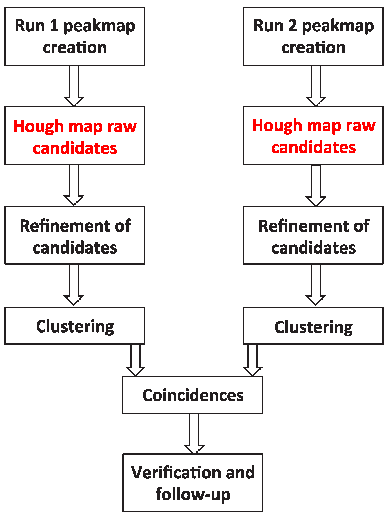
In this paper, we consider one of the standard search pipelines to search for CWs, that is, the mentioned FrequencyHough [7]. In particular we focus on the section that identifies the signal candidates and estimates their parameters, through an implementation of the so-called Hough transform (see Figure 1 which summarizes the core of the pipeline).
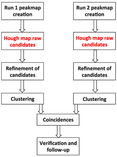
Figure 1.
A scheme that shows the steps of the full FrequencyHough pipeline. They are summarized in Section 2 and described in detail in [7]. The FrequencyHough transform and the candidate selection, highlighted in red, are the parts of the pipeline that have been ported on GPUs.
Briefly, the pipeline starts from a database of short Fourier transforms (FFT), computed from chunks of the data with a given duration [7]. The most significant peaks are selected in the equalized spectra from each FFT, producing a collection of time-frequency peaks that we refer to as peakmap. The peakmaps are stored in files that will be used as input for the FrequencyHough step of the pipeline, and they cover the full time of the detector observational run and a frequency interval of for and of for .
For every point in the sky, which is also discretized, the Doppler effect is corrected: a double sinusoidal pattern in the peakmap, due to the superposition of orbital and rotational Earth Doppler-shifts, becomes a straight line over the whole observation time.
The peaks are then fed to the FrequencyHough transform algorithm (for details see Section 2.1). This step of the analysis is crucial because it produces the set of candidates, that is, significant points in the signal frequency–frequency time derivative space, and represents the main computational burden of the whole pipeline. Once we have selected the candidates from both detectors, they are stored in files where their parameters are saved (sky coordinates, frequency, spindown), and this is the final output of the FrequencyHough transform step.
After the candidates collection and storage, their parameter space position is refined and their number is reduced, by clustering those below a certain distance in the parameter space and, most importantly, by matching the coincidence scheme between two or more detectors. The selected candidates are fed to a follow-up analysis in order to finally discard them or claim a detection [7].
2.1. Hough Transform
The FrequencyHough transform is a special implementation of CW searches of the so-called Hough transform, a pattern-recognition method [22] that was conceived for the study of subatomic particle tracks in bubble chambers, where curved tracks are divided, with good approximation, in sufficiently small line segments.
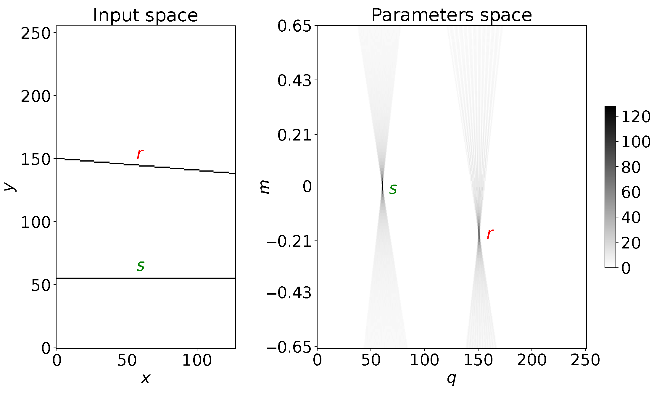
Considering an image where the line is formed by a series of co-linear black points with a pure white background, the detection of a track using the Hough transform consists of the transformation of the input image into another image (that we refer to as “the Hough map”), where a point with coordinates is converted into a straight line, whose slope and intercept are given by the point coordinates in the input image. If we take a sequence of points along a straight track with equation , they will be represented in the Hough map by straight lines with changing slopes and intercepts, forming an intersecting family of lines. The coordinates of the incidence point in the Hough space will be the parameter values of the line in the coordinate space (see Figure 2 for an example). Then, the Hough transform translates a straight line in the input coordinate space into points in the parameter space and allow us to measure the parameters of straight lines in the input images.
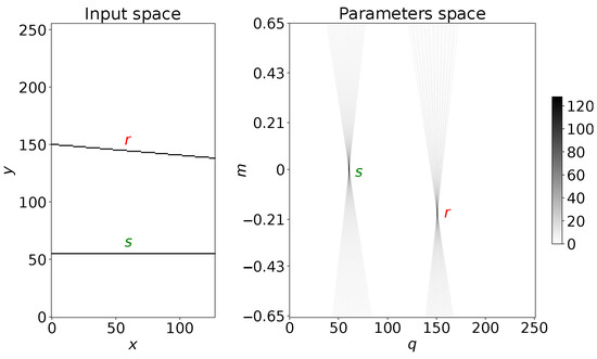
Figure 2.
Example of the Hough transform of two straight lines with different slopes. In the left plot, the lines are drawn in the x-y input plane, while in the right plot their parameters are shown as being computed by the Hough transform: each line in the input space is translated into a family of straight lines intersecting in their relative parameter space points.
Since we work with digitized images, the parameter space is discretized. The Hough map will then be a 2D histogram, where each pixel will have a count depending on how many lines are entered into that parameter space region. A given pixel in the map records the number of lines passing through it and the number count in each pixel will provide information on the significance of a point in the parameter space, within the error given by the image resolution (i.e., the bin sizes of the input space).
The Hough transform can be generalized in the following ways: (i) enhancing or reducing the resolution of the Hough map (to have either better precision on the parameter estimation or to reduce the computation load); (ii) using any N-dimensional manifold as input space and an M-dimensional manifold as parameter space, searching for curves rather than straight lines [23,24,25].
2.2. FrequencyHough Transform
The FrequencyHough transform is particularly well suited to searching for continuous gravitational waves [7,26]. As already stated, it starts with an input peakmap where the Doppler effect due to the Earth’s motion has been corrected. The transformation is from the peaks of the detector frequency/time plane to the gravitational wave frequency/spindown parameters plane.
With intrinsic frequency and spindown as parameters of a given neutron star waveform, and as an arbitrary reference time, the expected path in the peakmap at first order is given by the time law in Equation (2) [26]:
Keeping in mind that the frequency bins in the peakmap have a width , we enhance the resolution of the parameters in the FrequencyHough map by ten times: . A peakmap point is then transformed into a stripe between two parallel straight lines with a width given by the relation
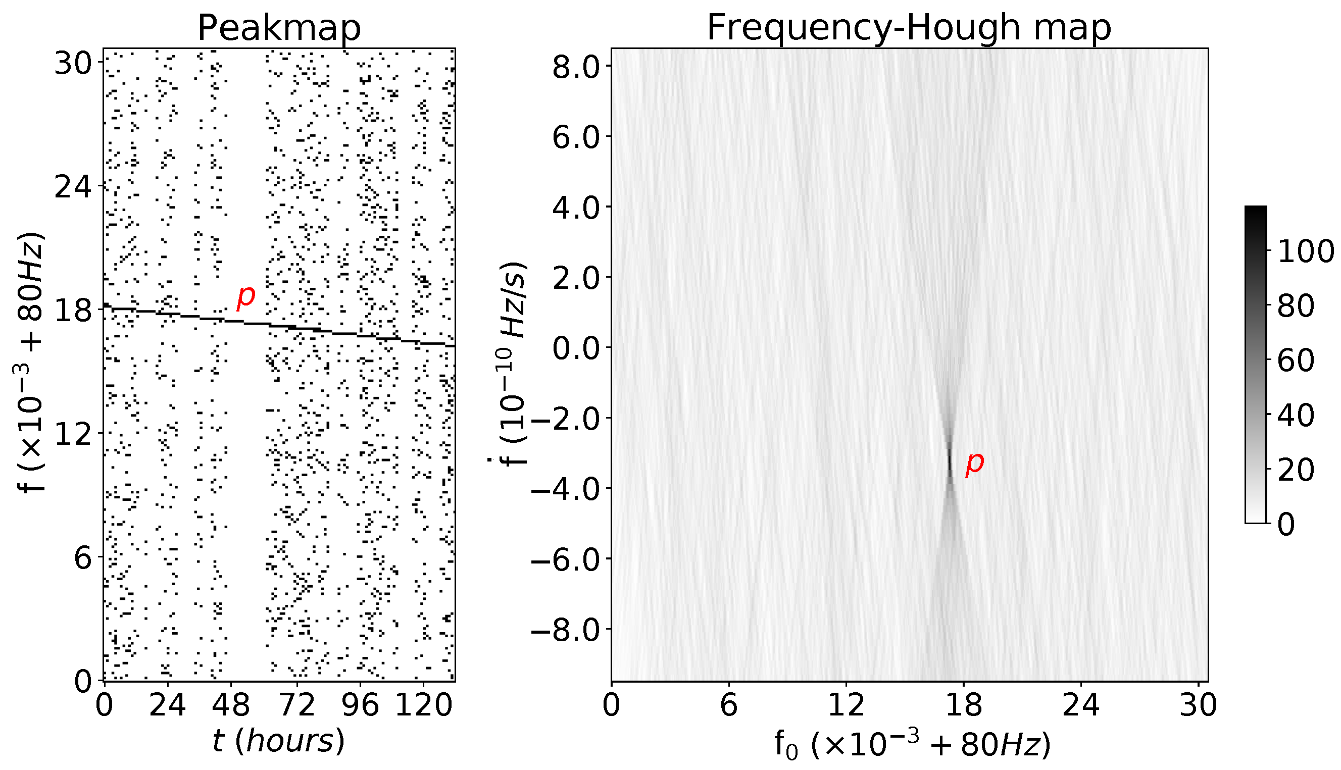
Then, for every row (i.e., along the spindown dimension), the FrequencyHough map is computed with a differential method: all the elements of one of the two edges, that is, those that match the relation , are increased by 1. Once this step is carried out, the elements on the other edge of the stripe are decreased by 1, straightforwardly using array slicing to immediately identify the elements matching (we just take the elements found in the first step and move by the number of bins corresponding to ). Finally, the row is cumulatively summed. An example is shown in Figure 3, where a straight line has been superimposed onto a portion of a peakmap and then the FrequencyHough has been run on it.
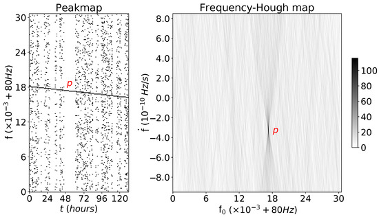
Figure 3.
Example of a peakmap with real data (from LIGO Livingston O2 run [27]) and a straight line superimposed directly on the peakmap to naively simulate a pulsar signal with reference frequency Hz taken at mid time period of the peakmap, and spindown parameter .
Exactly like the naive example in Figure 2, every point in the input is transformed into a straight line (in this case into a belt between two lines), and the aligned points of the straight line produce belts in the FrequencyHough map that converge in the parameters of the input line, allowing us to identify it when searching for the pixel in the FrequencyHough map with the highest number count.
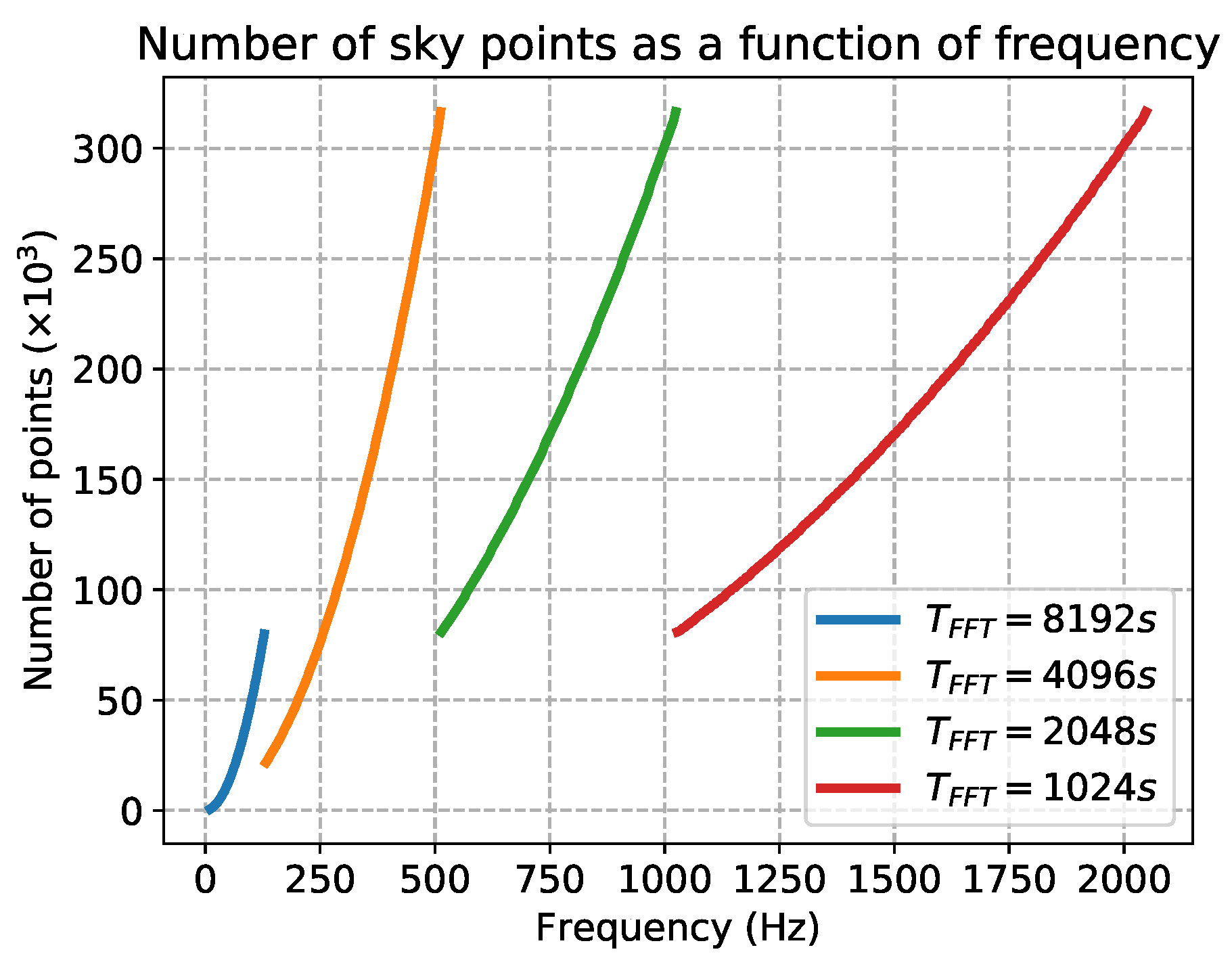
For all-sky searches, the size of the parameter space given by the sky grid is crucial. For each input peakamp, the number of sky points depend on its maximum frequency and on the FFT duration [7]. In Figure 4, we show the sky resolution versus the frequency for the four bands used for the standard FrequencyHough analysis.

Figure 4.
Plots of the number of points in the sky grid generated for the FrequencyHough search, as a function of frequency.
To cover all parameter space across the full frequency range, millions of core hours are necessary for a typical analysis over several months of data. GPU parallelism could support a significantly higher computation efficiency, allowing us to run a much deeper analyses.
3. General Purpose Computing on GPUs
A GPU is a device created and developed to perform computations with an extremely high parallelism and the best possible efficiency.
After very fast technological development, GPUs currently have hundreds and even thousands of cores and several GB of dedicated RAM: thanks to GPUs, the processing power for floating point calculations has exploded in the last ten years, and the use of GPUs in many different fields, from scientific research to economics and so on, gave birth to General Purpose computing on GPUs (GPGPU). At the present time, GPUs are no longer created with the sole purpose of building 3D animation, but specifically for big data computations, and GPUs for data centers dedicated to massive scientific calculations are an established reality. Within this context, with the creation of the CUDA [28] and OpenCL [29] frameworks, software development of algorithms for scientific research that is able to exploit the computation power of this new technology is finally affordable.
TensorFlow
TensorFlow [20] is a framework for high-level GPGPU programming that works with a symbolic paradigm and a syntax similar to high-level scientific programs/languages, such as Matlab [30], or numerical Python libraries like Numpy [31]. Despite having been originally developed for machine learning and neural networks, TensorFlow works well for a wide variety of purposes and, specifically, for scientific data analysis. The main reasons are that, apart from the neural network dedicated part, it has many functions for numerical computations, statistics and tensorial operations, which are developed to run very efficiently on GPUs with a high scalability for multi-GPU systems.
TensorFlow uses the dataflow paradigm, where a program is modeled as a graph of operations where the data flow through. The central units of data in TensorFlow are N-dimensional arrays called tensors. Operations on tensors are represented by nodes in a graph, while the edges are the input/output tensors, which link the operations of the flow.
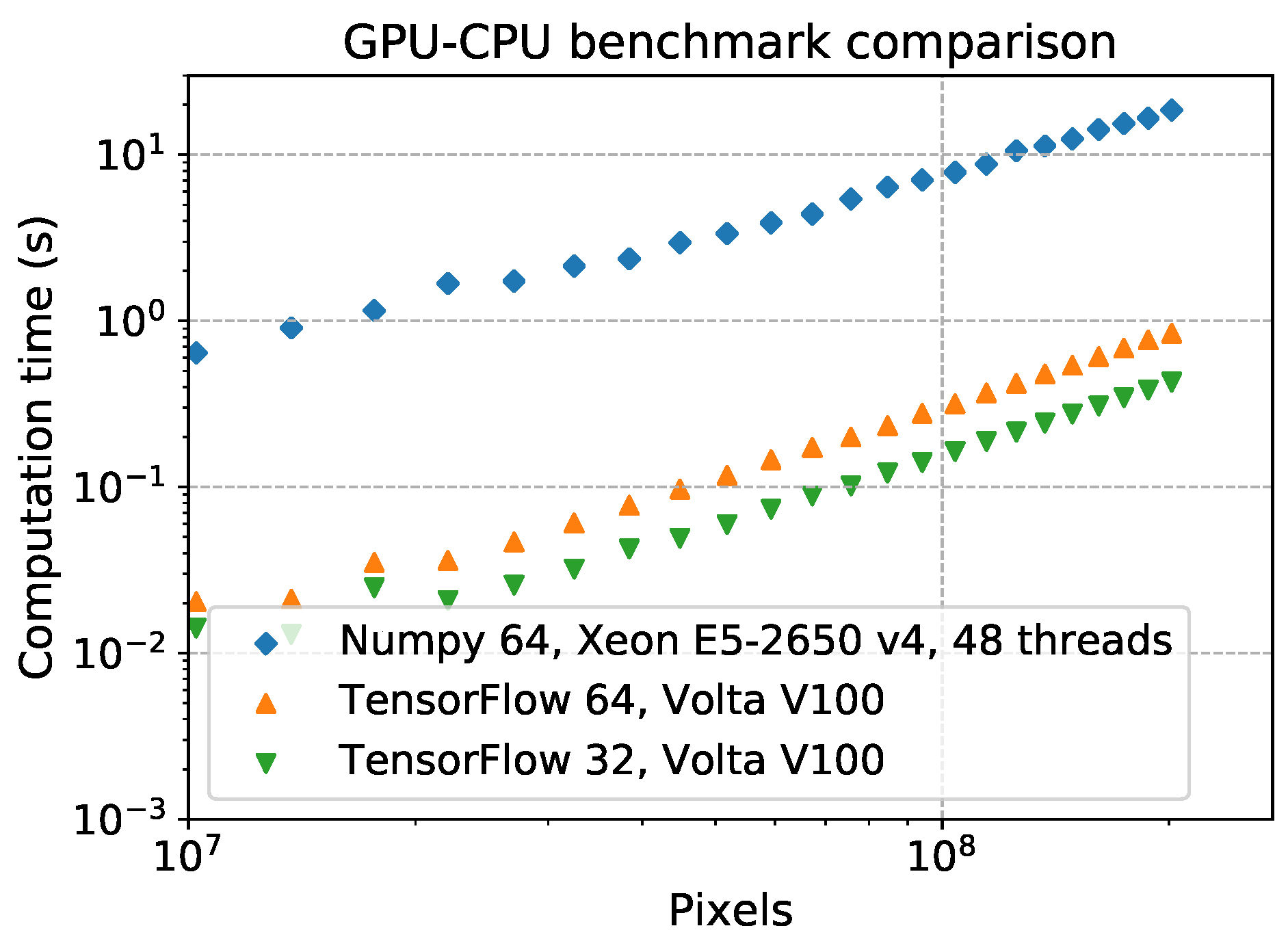
A simple example of the performance of TensorFlow on a single GPU, compared to Numpy on a single multi-thread CPU system, is shown in Figure 5, where the time execution of the random generation of two matrices with increasing size, and a matricial product between them, has been plotted. Taking into account that the used devices are not of the same class of performance, this example shows that, with well parallelizable algorithms, the improvement in performance using the GPU high-level TensorFlow functions can be up to one order of magnitude in terms of computation time.

Figure 5.
A simple benchmark on two example devices: an Intel Xeon E5-2650 v4 CPU system with, in total, 24 2.20 GHz cores and 48 threads, and a NVIDIA Volta V100 with 5120 cores at . The test is based on the generation of two random 2-rank arrays and a matrix multiplication between them. The green and orange dots show the benchmark conducted, respectively, with 64 and 32 bit data with TensorFlow, the blue ones come from a test with 64 bit data with Numpy. The test with the CPUs has been performed keeping the multithreading enabled as by default for Numpy.
All tests shown in this paper have been performed on the GPUs of the Cineca Marconi100 cluster [32] and on the CPUs of the LIGO–Caltech CIT cluster [33] (we refer readers to the institutional web pages for details of the hardware specifications).
4. FrequencyHough on TensorFlow
The standard FrequencyHough algorithm [7] is written in Matlab and is based on the SNAG toolbox [34]. The new code has been written in Python with TensorFlow APIs up to version 13.1, using CUDA libraries up to 10.01. The first step of the GPU porting has been to write a fully vectorized version of the code. This is a crucial step with high-level languages because, using a library with functions that are well developed and compiled in a low level language, the code will often be faster than a custom function with similar instructions or, even worse, loop cycles.
The greatest challenge in the GPU vectorization of the code has been the parallelization over the spindown values. Every spindown row in the FrequencyHough map algorithm is created independently. To limit the memory usage, we used a TensorFlow built-in function to map a single spindown iteration along the full search interval in a parallel and efficient way, rather than running a loop2. The integration part is instead intrinsically sequential, so it becomes rapidly the most inefficient part of the code when the frequency resolution is enhanced3.
Another delicate part of the analysis is the candidate selection. Once the FrequencyHough map for the selected sky positions has been generated, usually the matrix is split along the frequency dimension in an arbitrary number of vertical stripes, where the local maxima are selected [7]. The number of frequency stripes depends on how many candidates the search will produce; usually that number is fixed on 1 candidate for every .
We note that, in terms of programming languages, this can create some issues: if in a stripe there were more candidates with the same number count value but at different spindown values, the algorithm would select only the first occurrence, discarding the others. To bypass this technical limitation, we split the whole spindown range into different spindown sub-intervals and, for each of them, the candidate selection routine was run independently.
Thanks to the vectorization method used for the generation of the Hough map, with TensorFlow we can also naturally parallelize the candidate selection over the spindown sub-intervals, rather than running it sequentially. In this way, since increasing the number of sub-intervals makes the increase in computation time negligible, we can select more candidates, thus improving the search sensitivity.
Benchmarks
The GPU FrequencyHough code can run on devices that have enough memory and computational power like those built for big data centers, with a speed-up that can reach 1–2 orders of magnitude with respect to the standard code of [7], using the same input and parameter space. In Figure 6, we present an estimation of the running time of the GPU FrequencyHough code compared to the CPU version that runs on a single core. The bar plots for the different used in the analysis (which imply different sizes of the input peakmap) show that the FrequencyHough map computation—which was the dominating part of the execution time of the whole pipeline—thanks to the GPU function becomes lighter than the weighting process of the peakmaps, which is still running on CPUs, using Numpy functions with the multithreading enabled.
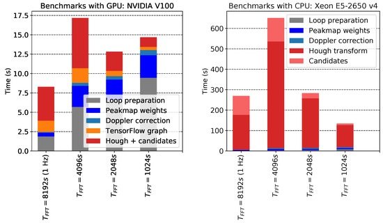
Figure 6.
Detailed comparison between the estimated running time of the GPU- (left plot) and the CPU- (right plot) based FrequencyHough codes. The grey part of the benchmark is executed only once per job and contributes negligibly to the overall cost, while the colored parts of the bars constitute one iteration over the sky positions and are in the main loop. The part where TensorFlow is involved has been split into two pieces: the graph building and variables initialization (orange) and the graph execution (red). The GPU code, after the TensorFlow graph is created, computes the FrequencyHough transform and the candidate selection at once, so it is not possible to split the two steps without the introduction of an overhead caused by the fact that the graph is generated and run in two steps. We remark that the CPU code can run only on a single thread. Hence, in the right plot we show the performance in terms of computing times using a single CPU core.
The porting was carried out and tested in order to return the same set of candidates of the original code. The peakmaps used for the benchmarks were generated with a time duration of 12 months; between and we have a peakmap for every , while for the other frequencies instead they cover a 5- band.
The spindown range is the same for each frequency band: . being the observation time, the spindown resolution is defined as . With this definition, we have, respectively, for the four datasets (see Table 1) the following number of spindown bins: 2566, 1284, 644, 322.

Table 1.
Frequency range and for the four frequency bands used in this analysis.
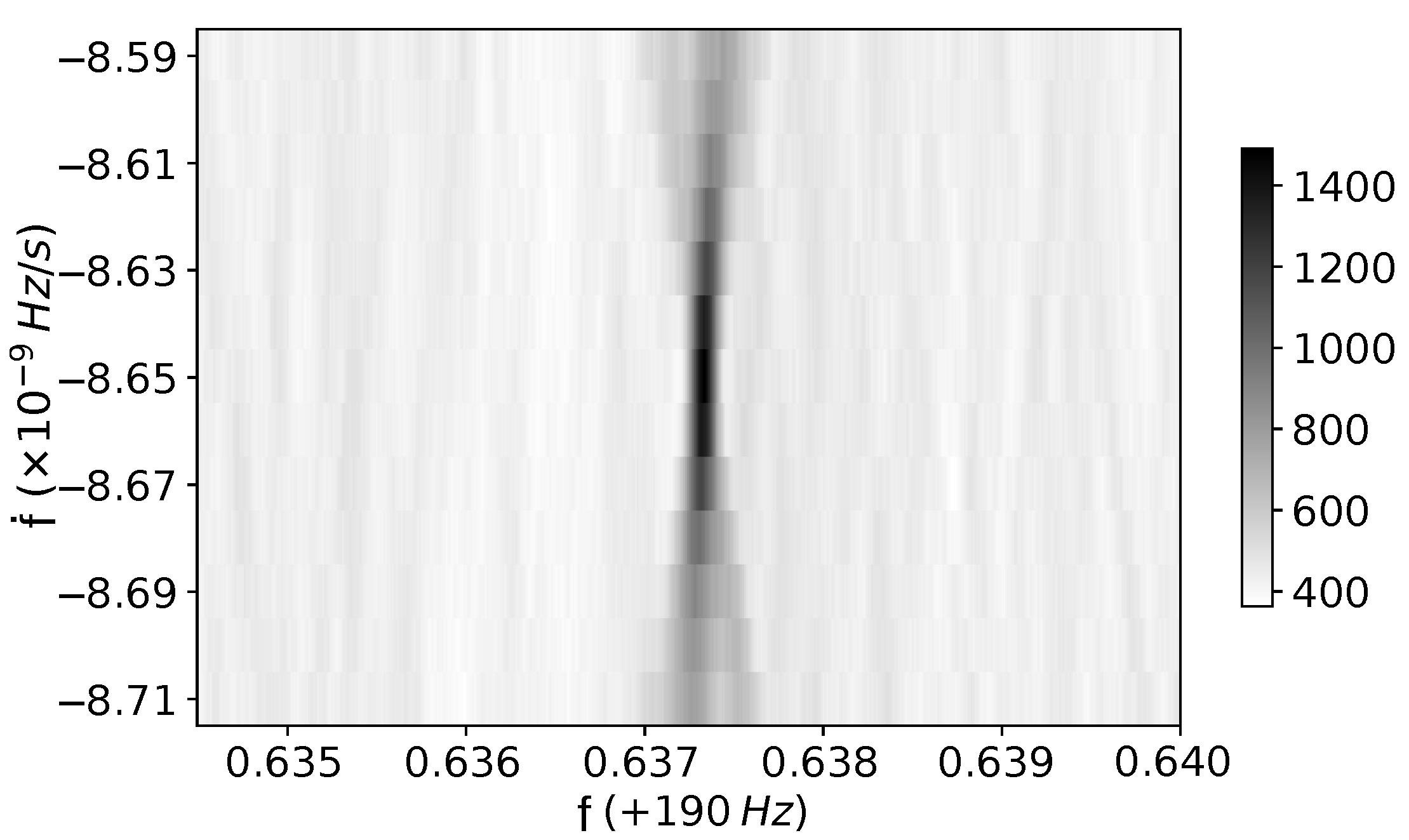
The devices used are an Intel Xeon E5-2650 v4 CPU with 24 2.20 GHz execution threads and a NVIDIA Volta V100 with 5120 cores at 1500 MHz and 16 GB of memory. An example of a FrequencyHough transform applied to a hardware injection in the data from the O2 run of the LIGO Hanford detector is shown in Figure 7.

Figure 7.
The GPU FrequencyHough algorithm applied to a hardware injection (so-called pulsar_8) in O2 LIGO Hanford data [27], with parameters: , Hz/s and ecliptic coordinates , .
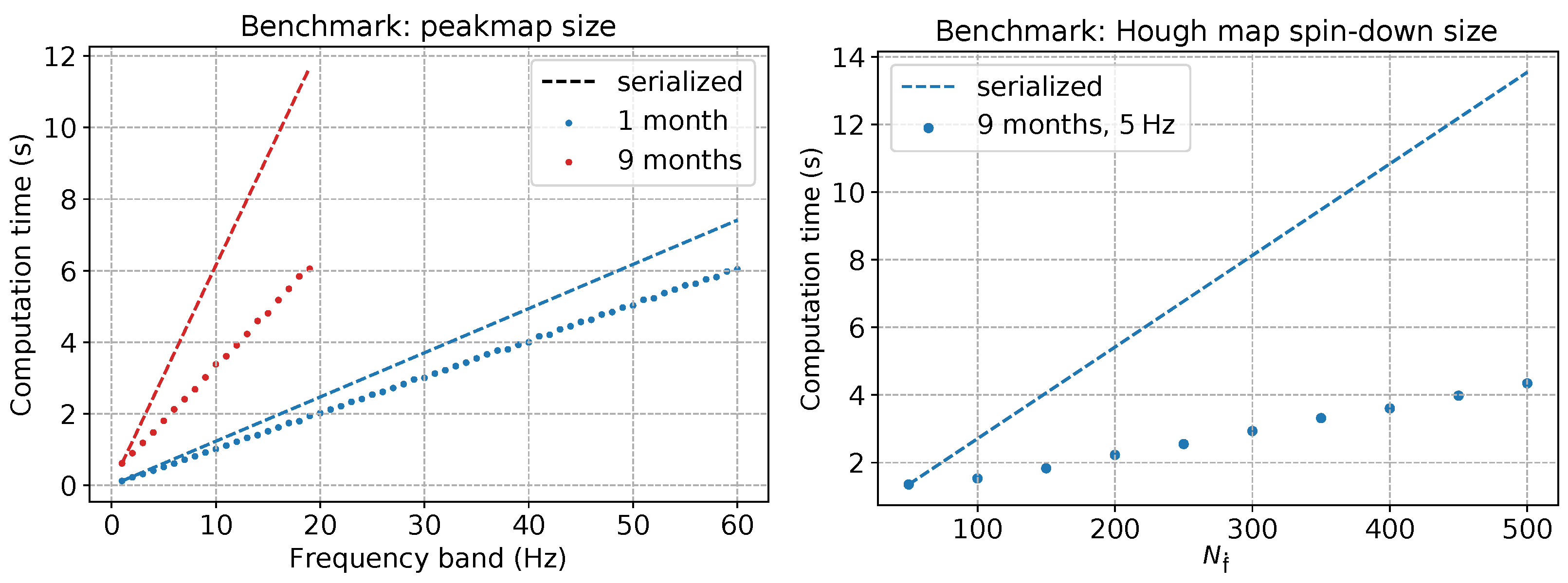
To provide better insight into how the performance of the code works with different sizes of the input time-frequency space and the frequency-spindown parameter space, we show in Figure 8 the results of another set of tests on the code efficiency: the parallelism efficiency of a GPU is well exploited when its memory and core architecture are filled as much as possible with parallelizable instructions.Due to this, the longer a given observation run is, the more efficient is the search with the new GPU code with respect to the older one.

Figure 8.
GPU tests for the FrequencyHough algorithm on a Tesla k20 (2496 cores at and 5 GB of memory) changing some key parameters: the size of the input (time interval–frequency range of the peakmap), and the size of the parameter space (number of spindown bins). The plots show the increasing efficiency of the GPU parallelism with a higher load on the memory and cores of the device. Left: computation time as a function of the frequency band covered by the peakmap. The measured computation times (dotted lines) are compared to those we would obtain by serializing the GPU code over peakmaps (dashed lines). The red plots show that, with a large peakmap, when the memory of the device is full, the efficiency of the parallelization halves the computation time needed for a separate analysis of 20 1 Hz large peakmaps. The blue plot comes from a 1 month long peakmap, with a time gain. Right: computation time as function of the number of spindown steps of the Hough map, with months and . Dotted and dashed lines have the same meaning as before. The plot shows a time reduction with respect to the serialized case, proving that the vectorization with TensorFlow is successful.
To provide an estimate of the different performances for a dataset spanning 1 year of observing time, 5 million CPU core hours are needed to complete a full all-sky analysis, while the pipeline equipped with the GPU FrequencyHough transform will take only ~130 thousand single-GPU hours.
5. Conclusions
In this work, we have shown the usefulness of GPGPU by developing analysis algorithms for the search for CWs. By parallelizing the FrequencyHough transform computation on GPUs, for a single Doppler corrected peakmap, we obtained a speed-up of the analysis by a factor of 10 in comparison to the original code. As seen in Figure 8, we also showed that by improving the degree of parallelism, that is, analyzing more data and a larger parameter space at once, the efficiency of the analysis can be increased further, by an amount that depends strongly on the devices used, but roughly by another ~.
With the computational speed of the GPUs, other portions of the pipeline that run on CPUs become the bottleneck of the pipeline, and should be ported on GPUs as well. By updating the code to the newer versions of TensorFlow, the time that TensorFlow takes to generate and initialize the graph is also expected to be reduced.
With the better performances granted to a well developed GPGPU code, one can consider adding higher order spindown parameters and expanding the parameter space in order to increase the probability of a detection. To this purpose, a few arrangements and improvements could be made, such as:
- Extend the code to run on multi-GPU systems, exploiting the larger memory to load and process larger files at once;
- Develop a scalable big data input/output pipeline, which can work out-of-memory, using appropriate modern file formats and libraries, trying to balance serialization and parallelism.
The field of big data computation with GPUs is fast evolving, with new hardware architectures that raise the available computational power, and an increasing number of frameworks, which allow us to develop codes with a high variety of purposes. Due to this, we expect that an increasing amount of scientific analysis in the next years will use such devices and frameworks. Thanks to the availability of clusters made by thousands of data center GPUs, it has become crucial to have codes that can efficiently exploit the computational power of these devices.
Developing GPGPU codes for CW searches is thus of primary importance.
Author Contributions
Conceptualization, I.L.R., P.A., S.F. and C.P.; Data curation, P.L. and O.J.P.; Formal analysis, I.L.R.; Funding acquisition, P.L. and T.R.; Methodology, I.L.R.; Resources, P.A. and C.P.; Software, I.L.R., P.A. and S.F.; Supervision, P.A., P.L., C.P. and T.R.; Validation, P.A. and C.P.; Visualization, I.L.R.; Writing—original draft, I.L.R.; Writing—review & editing, P.A., S.D., S.F., P.L., A.L.M., C.P., O.J.P., L.P. and T.R. All authors have read and agreed to the published version of the manuscript.
Funding
This research was funded by European Gravitational Observatory as part of the PhD scholarship of I.L.R.
Data Availability Statement
The data presented in this study are openly available in Gravitational Wave Open Science Center at doi:10.1016/j.softx.2021.100658.
Acknowledgments
We thank the LIGO Scientific Collaboration for access to LIGO data, as well as the funding agencies that enabled the construction and operation of the LIGO observatories.This material is based upon work supported by NSF’s LIGO Laboratory which is a major facility fully funded by the National Science Foundation. We also acknowledge the support of the CIT cluster, Cineca and CNAF, and we acknowledge the European Gravitational Observatory for funding this project.
Conflicts of Interest
The authors declare no conflict of interest.
Notes
| 1 | An update to TensorFlow 2.x with CUDA 11.x is planned in the near future. |
| 2 | The function used is map_fn: it applies a function along elements of a tensor, parallelizing the instructions over the GPUs. |
| 3 | For this part, TensorFlow APIs have a cumulative sum function called cumsum. |
References
- Einstein, A. Näherungsweise Integration der Feldgleichungen der Gravitation. Sitzungsberichte Königlich Preußischen Akad. Wiss. 1916, 1, 688. [Google Scholar]
- Einstein, A. Über Gravitationswellen. Sitzungsberichte Königlich Preußischen Akad. Wiss. 1918, 1, 154. [Google Scholar]
- Abbott, B.P. et al. [LIGO Scientific Collaboration and Virgo Collaboration] Observation of gravitational waves from a binary black hole merger. Phys. Rev. Lett. 2016, 116, 061102. [Google Scholar] [CrossRef]
- Abbott, B.P. et al. [LIGO Scientific Collaboration and Virgo Collaboration] GW170817: Observation of gravitational waves from a binary neutron star inspiral. Phys. Rev. Lett. 2017, 119, 161101. [Google Scholar] [CrossRef] [PubMed] [Green Version]
- Abbott, B.P. et al. [LIGO Scientific Collaboration and Virgo Collaboration] GW170814: A three-detector observation of gravitational waves from a binary black hole coalescence. Phys. Rev. Lett. 2017, 119, 141101. [Google Scholar] [CrossRef] [PubMed] [Green Version]
- Abbott, B.P. et al. [LIGO Scientific Collaboration and Virgo Collaboration] All-sky search for continuous gravitational waves from isolated neutron stars using Advanced LIGO O2 data. Phys. Rev. D 2019, 100, 024004. [Google Scholar] [CrossRef] [Green Version]
- Astone, P.; Colla, A.; D’Antonio, S.; Frasca, S.; Palomba, C. Method for all-sky searches of continuous gravitational wave signals using the frequency-Hough transform. Phys. Rev. D 2014, 90, 042002. [Google Scholar] [CrossRef] [Green Version]
- Leaci, P.; Astone, P.; D’Antonio, S.; Frasca, S.; Palomba, C.; Piccinni, O.; Mastrogiovanni, S. Novel directed search strategy to detect continuous gravitational waves from neutron stars in low-and high-eccentricity binary systems. Phys. Rev. D 2017, 95, 122001. [Google Scholar] [CrossRef] [Green Version]
- Maggiore, M. Gravitational Waves: Volume 1: Theory and Experiments; Oxford University Press: Oxford, UK, 2008. [Google Scholar] [CrossRef]
- Ushomirsky, G.; Cutler, C.; Bildsten, L. Deformations of accreting neutron star crusts and gravitational wave emission. Mon. Not. R. Astron. Soc. 2000, 319, 902. [Google Scholar] [CrossRef] [Green Version]
- Cutler, C. Gravitational waves from neutron stars with large toroidal B fields. Phys. Rev. D 2002, 66, 084025. [Google Scholar] [CrossRef] [Green Version]
- Owen, B.J.; Lindblom, L.; Cutler, C.; Schutz, B.F.; Vecchio, A.; Andersson, N. Gravitational waves from hot young rapidly rotating neutron stars. Phys. Rev. D 1998, 58, 084020. [Google Scholar] [CrossRef] [Green Version]
- Bildsten, L. Gravitational radiation and rotation of accreting neutron stars. Astrophys. J. 1998, 501, L89. [Google Scholar] [CrossRef] [Green Version]
- Andersson, N.; Kokkotas, K.D.; Stergioulas, N. On the relevance of the r-mode instability for accreting neutron stars and white dwarfs. Astrophys. J. 1999, 516, 307. [Google Scholar] [CrossRef]
- Stairs, I.H.; Lyne, A.G.; Shemar, S.L. Evidence for free precession in a pulsar. Nature 2000, 406, 484. [Google Scholar] [CrossRef]
- Australia Telescope National Facility. The ATNF Pulsar Catalogue. 2021. Available online: http://www.atnf.csiro.au/people/pulsar/psrcat/ (accessed on 29 June 2021).
- Bisnovatyi-Kogan, G.S. The neutron star population in the Galaxy. Int. Astron. Union. Symp. 1992, 149, 379. [Google Scholar] [CrossRef]
- Palomba, C. The search for continuous gravitational waves in LIGO and Virgo data. Nuovo Cim. 2017, 40, 129. [Google Scholar] [CrossRef]
- Sieniawska, M.; Bejger, M. Continuous gravitational waves from neutron stars: Current status and prospects. Universe 2019, 5, 217. [Google Scholar] [CrossRef] [Green Version]
- The TensorFlow Authors, TensorFlow. 2021. Available online: www.tensorflow.org (accessed on 29 June 2021).
- Saulson, P.R. Fundamentals of Interferometric Gravitational Wave Detectors; World Scientific: Singapore, 2017. [Google Scholar] [CrossRef] [Green Version]
- Hough, P.V.C. Method and Means for Recognizing Complex Patterns. U.S. Patent No. 3069654, 18 December 1962. [Google Scholar]
- Duda, R.O.; Hart, P.E. Use of the Hough transformation to detect lines and curves in pictures. Commun. ACM 1972, 15, 11. [Google Scholar] [CrossRef]
- Ballard, D.H. Generalizing the Hough transform to detect arbitrary shapes. Pattern Recognit. 1981, 13, 111. [Google Scholar] [CrossRef] [Green Version]
- Miller, A.; Astone, P.; D’Antonio, S.; Frasca, S.; Intini, G.; La Rosa, I.; Leaci, P.; Mastrogiovanni, S.; Muciaccia, F.; Palomba, C.; et al. Method to search for long duration gravitational wave transients from isolated neutron stars using the generalized frequency-Hough transform. Phys. Rev. D 2018, 98, 102004. [Google Scholar] [CrossRef] [Green Version]
- Antonucci, F.; Astone, P.; D’Antonio, S.; Frasca, S.; Palomba, C. Detection of periodic gravitational wave sources by Hough transform in the f versus f plane. Class. Quant. Grav. 2008, 25, 184015. [Google Scholar] [CrossRef] [Green Version]
- Abbott, R. et al. [LIGO Scientific Collaboration and Virgo Collaboration] Open data from the first and second observing runs of Advanced LIGO and Advanced Virgo. SoftwareX 2021, 13, 100658. [Google Scholar] [CrossRef]
- NVIDIA Corporation, CUDA Toolkit. 2021. Available online: https://developer.nvidia.com/cuda-toolkit (accessed on 29 June 2021).
- The Khronos Group, OpenCL. 2021. Available online: https://www.khronos.org/opencl (accessed on 29 June 2021).
- MathWorks, MATLAB. 2021. Available online: https://www.mathworks.com/products/matlab.html (accessed on 29 June 2021).
- Scipy Developers, Scipy. 2021. Available online: https://www.scipy.org (accessed on 29 June 2021).
- Cineca, Marconi100. 2021. Available online: https://www.hpc.cineca.it/hardware/marconi100 (accessed on 29 June 2021).
- LIGO Caltech, CIT. 2021. Available online: https://www.ligo.caltech.edu/ (accessed on 29 June 2021).
- Frasca, S. SNAG. 2018. Available online: https://www.roma1.infn.it/~frasca/snag/default.htm (accessed on 29 June 2021).

Publisher’s Note: MDPI stays neutral with regard to jurisdictional claims in published maps and institutional affiliations. |
© 2021 by the authors. Licensee MDPI, Basel, Switzerland. This article is an open access article distributed under the terms and conditions of the Creative Commons Attribution (CC BY) license (https://creativecommons.org/licenses/by/4.0/).