Article

Hints for a Gravitational Transition in Tully–Fisher Data

by
George Alestas
,
Ioannis Antoniou
and
Leandros Perivolaropoulos
*
Department of Physics, University of Ioannina, 45110 Ioannina, Greece
*
Author to whom correspondence should be addressed.
Universe 2021, 7(10), 366; https://doi.org/10.3390/universe7100366
Submission received: 2 September 2021 / Revised: 22 September 2021 / Accepted: 23 September 2021 / Published: 29 September 2021
(This article belongs to the Section Cosmology)

Abstract

:
We use an up-to-date compilation of Tully–Fisher data to search for transitions in the evolution of the Tully–Fisher relation. Using an up-to-date data compilation, we find hints at 3 σ level for a transition at critical distances D c 9 Mpc and D c 17 Mpc. We split the full sample in two subsamples, according to the measured galaxy distance with respect to splitting distance D c , and identify the likelihood of the best-fit slope and intercept of one sample with respect to the best-fit corresponding values of the other sample. For D c 9 Mpc and D c 17 Mpc, we find a tension between the two subsamples at a level of Δ χ 2 > 17 ( 3.5 σ ) . Using Monte Carlo simulations, we demonstrate that this result is robust with respect to random statistical and systematic variations of the galactic distances and is unlikely in the context of a homogeneous dataset constructed using the Tully–Fisher relation. If the tension is interpreted as being due to a gravitational strength transition, it would imply a shift in the effective gravitational constant to lower values for distances larger than D c by Δ G G 0.1 . Such a shift is of the anticipated sign and magnitude but at a somewhat lower distance (redshift) than the gravitational transition recently proposed to address the Hubble and growth tensions ( Δ G G 0.1 at the transition redshift of z t 0.01 ( D c 40 Mpc)).

1. Introduction

The Tully–Fisher relation (TFR) [1] has been proposed as an empirical relation that connects the intrinsic optical luminosity of spiral galaxies with their observed maximum velocity v r o t in the rotation curve as follows:
L = A v r o t s
where s 4 is the slope in a logarithmic plot of (1), and A is a constant ( l o g ( A ) is the zero point or intercept). The constants s and A appear to depend very weakly on galaxy properties, including the mass to light ratio, the observed surface brightness, the galactic profiles, H I gas content, size, etc. [2]. They clearly also depend, however, on the fundamental properties of gravitational interactions as demonstrated below.
The baryonic Tully–Fisher relation (BTFR) is similar to Equation (1) but connects the galaxy’s total baryonic mass (the sum of mass in stars and H I gas) M B with the rotation velocity as follows:
M B = A B v r o t s
where A B 50 M km 4 s 4 [3]. This allows to include gas-rich dwarf galaxies that appear in groups and have stellar masses below 10 9 M .
A simple heuristic analytical derivation for the BTFR can be obtained as follows [4]. Consider a star in a circular orbit of radius R around a galactic mass M rotating with velocity v. Then, the following holds:
v 2 = G eff M / R v 4 = ( G eff M / R ) 2 M S G eff 2
where G eff is the effective Newton’s constant involved in gravitational interactions and S the surface density S M / R 2 , which is expected to be constant [5]. From Equations (2) and (3), the following is anticipated:
A B G eff 2 S 1
Therefore, the BTFR can, in principle, probe both galaxy formation dynamics (through, e.g., S) and possible fundamental constant dynamics (through G eff ). An interesting feature of the BTFR is that despite the above heuristic derivation, it appears to be robust, even in cases when the galaxy sample includes low S and/or varying S galaxies [6,7]. In fact, no other parameter appears to be significant in the BTFR.
The BTFR has been shown to have lower scatter [2,8,9] than the classic stellar TFR and also to be applicable for galaxies with stellar masses lower than 10 9 M . It is also more robust than the classic TFR [10,11,12,13] since the parameters A B (intercept) and s (slope) are very weakly dependent on galactic properties, such as size and surface brightness [2].
The low scatter of the BTFR and its robustness make it useful as a distance indicator for the measurement of the Hubble constant H 0 . A calibration of the BTFR using Cepheid and TRGB distances leads to a value of H 0 = 75 ± 3.8 km s 1 Mpc 1 [14].
This value of H 0 is consistent with local measurements of H 0 , using SnIa calibrated with Cepheids ( H 0 = 73.2 ± 1.3 km s 1 Mpc 1 ) [15], but is in tension with the value of H 0 obtained using the early time sound horizon standard ruler calibrated using the CMB anisotropy spectrum in the context of the standard Λ CDM model ( H 0 = 67.36 ± 0.54 km s 1 Mpc 1 ) [16]. The tension between the CMB and Cepheid calibrators is at a level larger than 4 σ and constitutes a major problem for modern cosmologies (for a recent review and approaches see Refs. [17,18,19,20,21]).
The Hubble tension may also be viewed as an inconsistency between the value of the standardized SnIa absolute magnitude M calibrated using Cepheids in the redshift range 0 < z < 0.01 (distance ladder calibration) and the corresponding M value calibrated using the recombination sound horizon (inverse distance ladder calibration) for 0.01 < z < z r e c . Thus, a recently proposed class of approaches to the resolution of the Hubble tension involves a transition [22,23] of the standardized intrinsic SnIa luminosity L and absolute magnitude M at a redshift z t 0.01 from M = ( 19.24 ± 0.037 ) m a g for z < z t (as implied by Cepheid calibration) to M = ( 19.4 ± 0.027 ) m a g for z > z t (as implied by CMB calibration of the sound horizon at decoupling) [24]. Such a transition may occur due to a transition in the strength of the gravitational interactions G eff , which modifies the SnIa intrinsic luminosity L by changing the value of the Chandrasekhar mass. The simplest assumption leads to L M C h G eff 3 / 2 [25,26], even though corrections may be required to the above simplistic approach [27].
The weak evolution and scatter of the BTFR can be used as a probe of galaxy formation models as well as a probe of possible transitions of fundamental properties of gravitational dynamics since the zero point constant A B is inversely proportional to the square of the gravitational constant G. Previous studies investigating the evolution of the best-fit zero point l o g A B and slope s of the BTFR have found a mildly high z evolution of the zero point from z 0.9 to z 2.3 [28], which was attributed to the galactic evolution inducing a lower gas fraction at low redshifts after comparing with the corresponding evolution of the stellar TFR (STFR), which ignores the contribution of gas in the galactic masses.
Ref. [28] and other similar studies assumed a fixed strength of fundamental gravitational interactions and made no attempt to search for sharp features in the evolution of the zero point. In addition, they focused on the comparison of high redshift with low redshift effects without searching for possible transitions within the low z spiral galaxy data. Such transitions, if present, would be washed out and hidden from these studies, due to averaging effects. In the present analysis, we search for transition effects in the BTFR at z 0.01 (distances D 40 Mpc ), which may be due to either astrophysical mechanisms or to a rapid transition in the strength of the gravitational interactions G eff , due to fundamental physics.
In many modified gravity theories, including scalar tensor theories, the strength of gravitational interactions G eff measured in Cavendish-type experiments measuring force F between masses ( F = G eff m 1 m 2 r 2 ), is distinct from the Planck mass corresponding to G N that determines the cosmological background expansion rate ( H 2 = 8 π G N 3 ρ t o t ).
For example, in scalar tensor theories involving a scalar field ϕ and a non-minimal coupling F ( ϕ ) of the scalar field to the Ricci scalar in the Lagrangian, the gravitational interaction strength is as follows [29]:
G eff = 1 F 2 F + 4 F ϕ 2 2 F + 3 F ϕ 2
while the Planck mass related G N is as follows:
G N = 1 F
Most current astrophysical and cosmological constraints on Newton’s constant constrain the time derivative of G eff at specific times, assume a smooth power–law evolution of G eff , or constrain changes of the Planck mass–related G N instead of G eff (CMB and nucleosynthesis constraints [30]). Therefore, these studies are less sensitive in the detection of rapid transitions of G eff at low z.
The current constraints on the evolution of G eff and G N are summarized in Table 1, where we review the experimental constraints from local and cosmological time scales on the time variation of the gravitational constant. The methods are based on very diverse physics, and the resulting upper bounds differ by several orders of magnitude. Most constraints are obtained from systems in which gravity is non-negligible, such as the motion of the bodies of the solar system, and the astrophysical and cosmological systems. They are mainly related in the comparison of a gravitational time scale, e.g., period of orbits, with a non-gravitational time scale. One can distinguish between two types of constraints, from observations on cosmological scales and on local (inner galactic or astrophysical) scales. The strongest constraints to date come from lunar ranging experiments.
In the first column of Table 1, we list the used method. The second column contains the upper bound | Δ G G | m a x of the fractional change of G during the corresponding timescale. Most of these bounds assume a smooth evolution of G. In the third column, we present the upper bound on the normalized time derivative | G ˙ G | m a x . The fourth column is an approximate time scale over which each experiment is averaging each variation, and the fifth column refers to the corresponding study where the bound appears. Entries with a star (*) indicate constraints on G N , while the rest of the constraints refer to the gravitational interaction constant G eff .
In the present analysis, we search for a transition of the BTFR best-fit parameter values (intercept and slope) between data subsamples at low and high distances. We consider sample dividing distances D c [ 2 , 60 ] Mpc , using a robust BTFR dataset [12,31,32,33], which consists of 118 carefully selected BTFR datapoints, providing distance, rotation velocity baryonic mass ( D , V f , M B ) as well as other observables with their 1 σ errorbars. We focus on the gravitational strength Newton constant G eff and address the following questions:
  • Are there hints for a transition in the evolution of the BTFR?
  • What constraints can be imposed on a possible G eff transition, using BTFR data?
  • Are these constraints consistent with the level of G eff required to address the Hubble tension?
The structure of this paper is the following: In the next section, we describe the datasets involved in our analysis and present the method used to identify transitions in the evolution of the BTFR at low z. We also show the results of our analysis. In Section 3, we summarize, present our conclusions and discuss possible implications and extensions of our analysis.
Table 1. Solar system, astrophysical and cosmological constraints on the evolution of the gravitational constant. Methods with star (*) constrain G N , while the rest constrain G eff . The latest and strongest constraints are shown for each method.
Method | Δ G eff G eff | max | G ˙ eff G eff | max ( yr 1 )Time Scale (Yr)References
Lunar ranging 1.47 × 10 13 24[34]
Solar system 4.6 × 10 14 50[35,36]
Pulsar timing 3.1 × 10 12 1.5[37]
Strong Lensing 10 2 0.6[38]
Orbits of binary pulsar 1.0 × 10 12 22[39]
Ephemeris of Mercury 4 × 10 14 7[40]
Exoplanetary motion 10 6 4[41]
Hubble diagram SnIa0.1 1 × 10 11 10 8 [42]
Pulsating white-dwarfs 1.8 × 10 10 0[43]
Viking lander ranging 4 × 10 12 6[44]
Helioseismology 1.6 × 10 12 4 × 10 9 [45]
Gravitational waves8 5 × 10 8 1.3 × 10 8 [46]
Paleontology 0.1 2 × 10 11 4 × 10 9 [47]
Globular clusters 35 × 10 12 10 10 [48]
Binary pulsar masses 4.8 × 10 12 10 10 [49]
Gravitochemical heating 4 × 10 12 10 8 [50]
Strong lensing 3 × 10 1 10 10 [38]
Big Bang Nucleosynthesis * 0.05 4.5 × 10 12 1.4 × 10 10 [30]
Anisotropies in CMB * 0.095 1.75 × 10 12 1.4 × 10 10 [51]

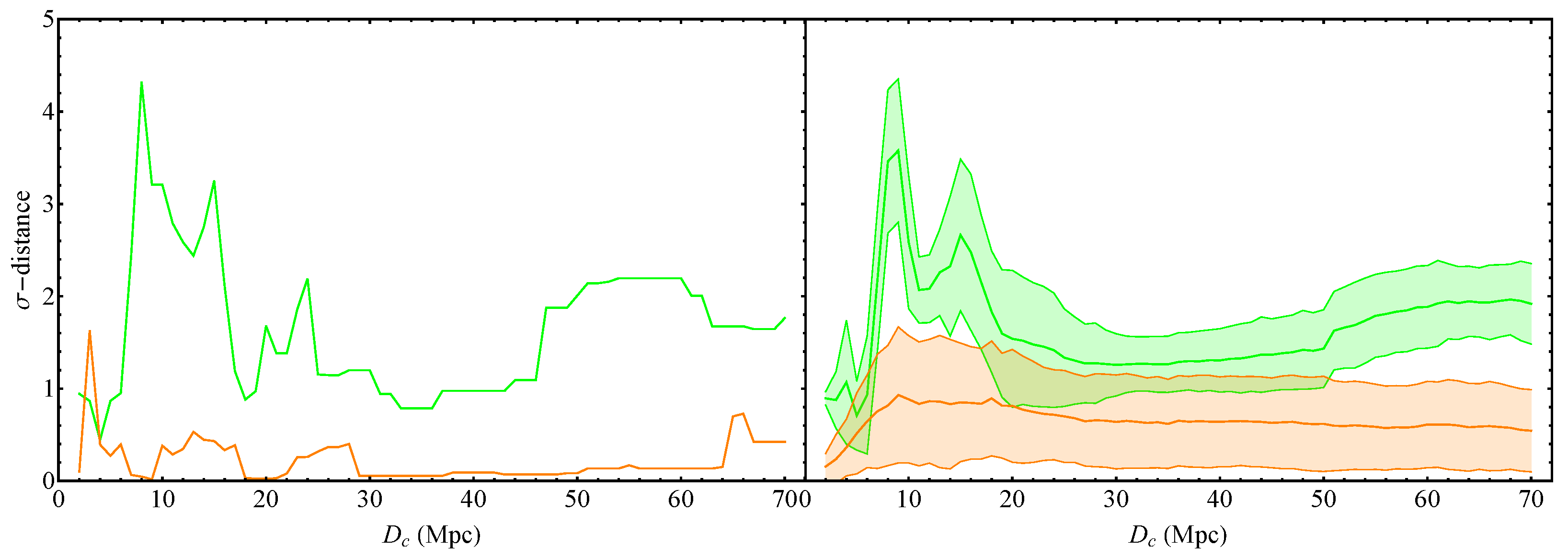
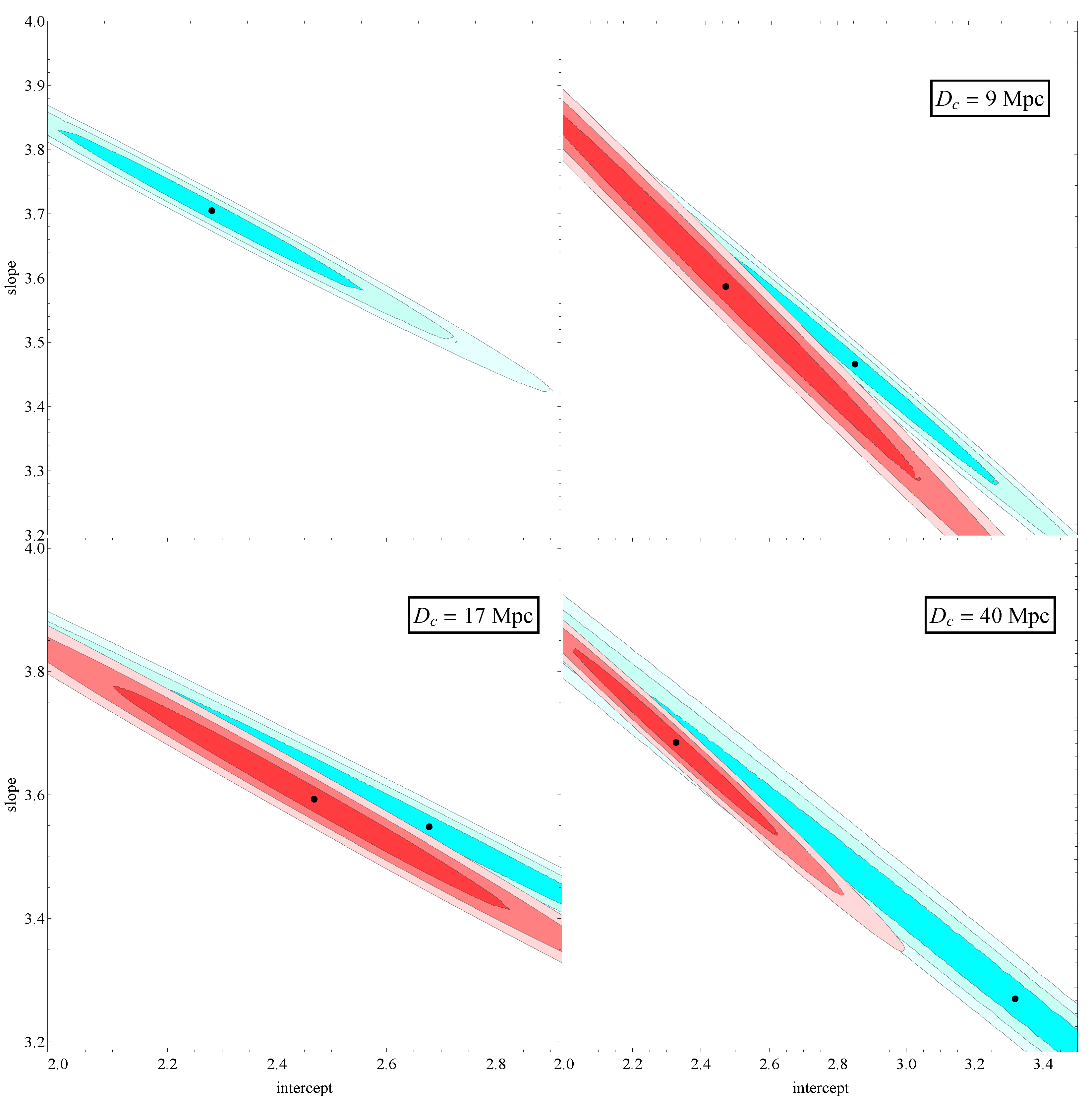
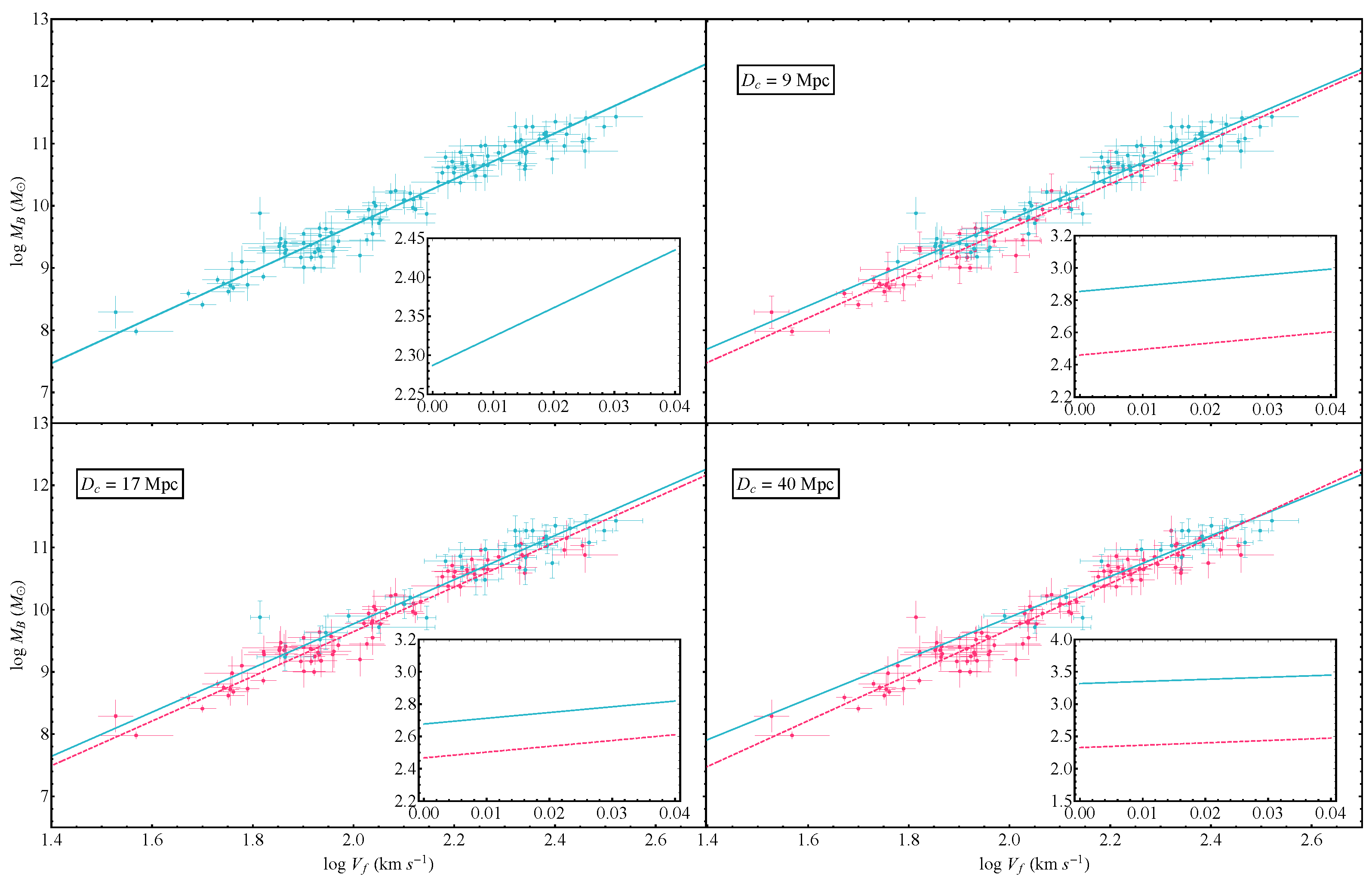
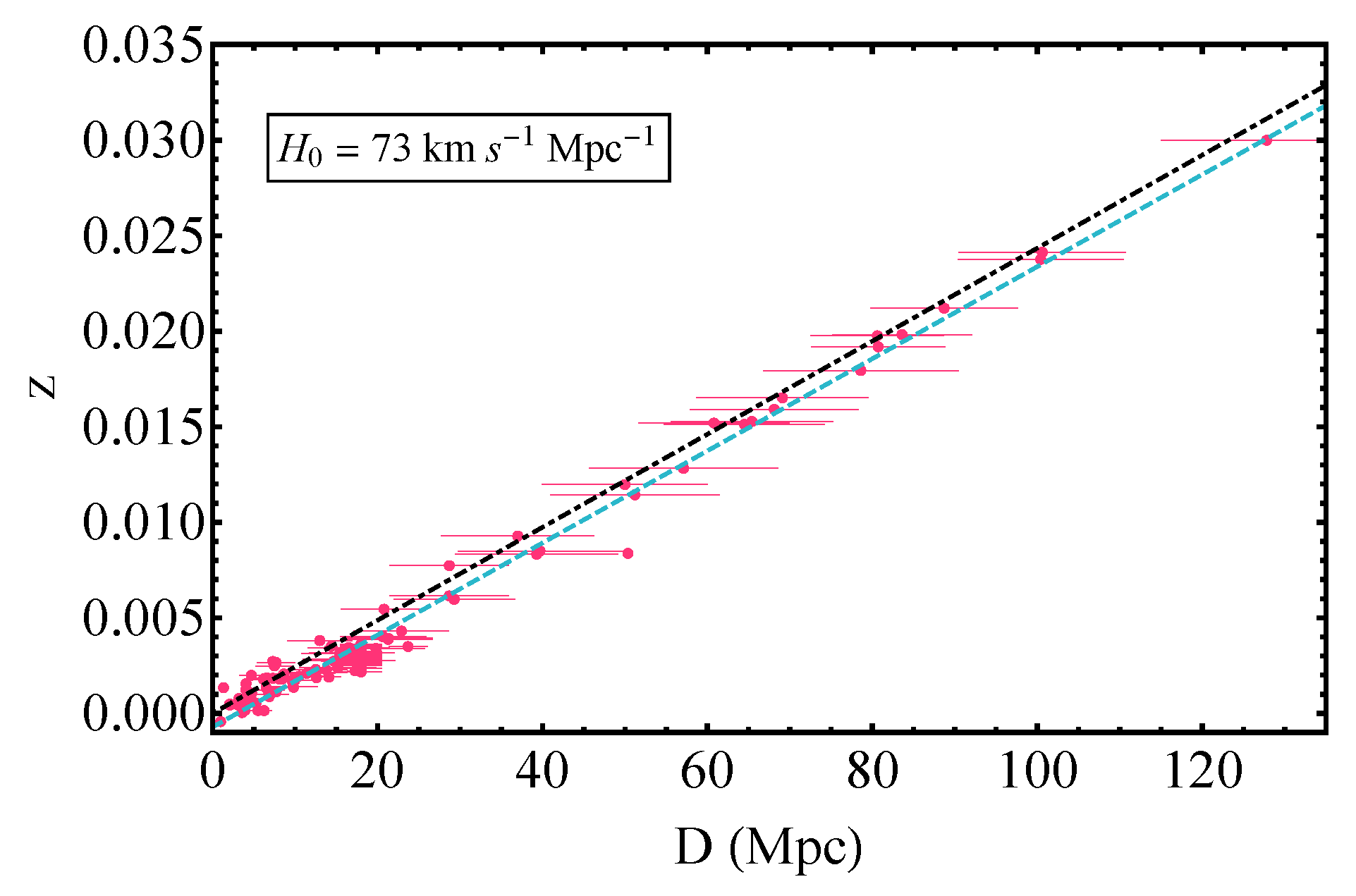
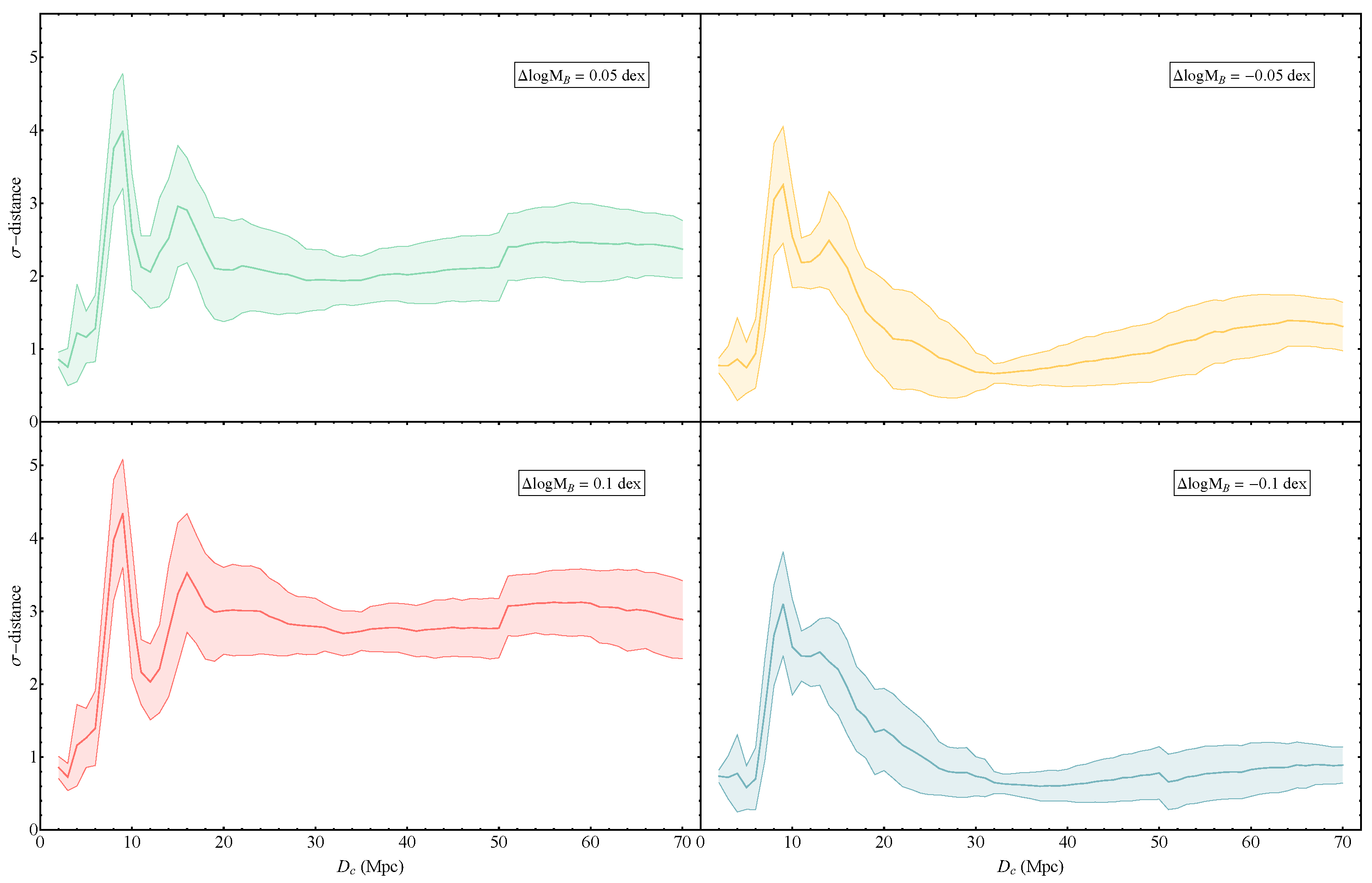
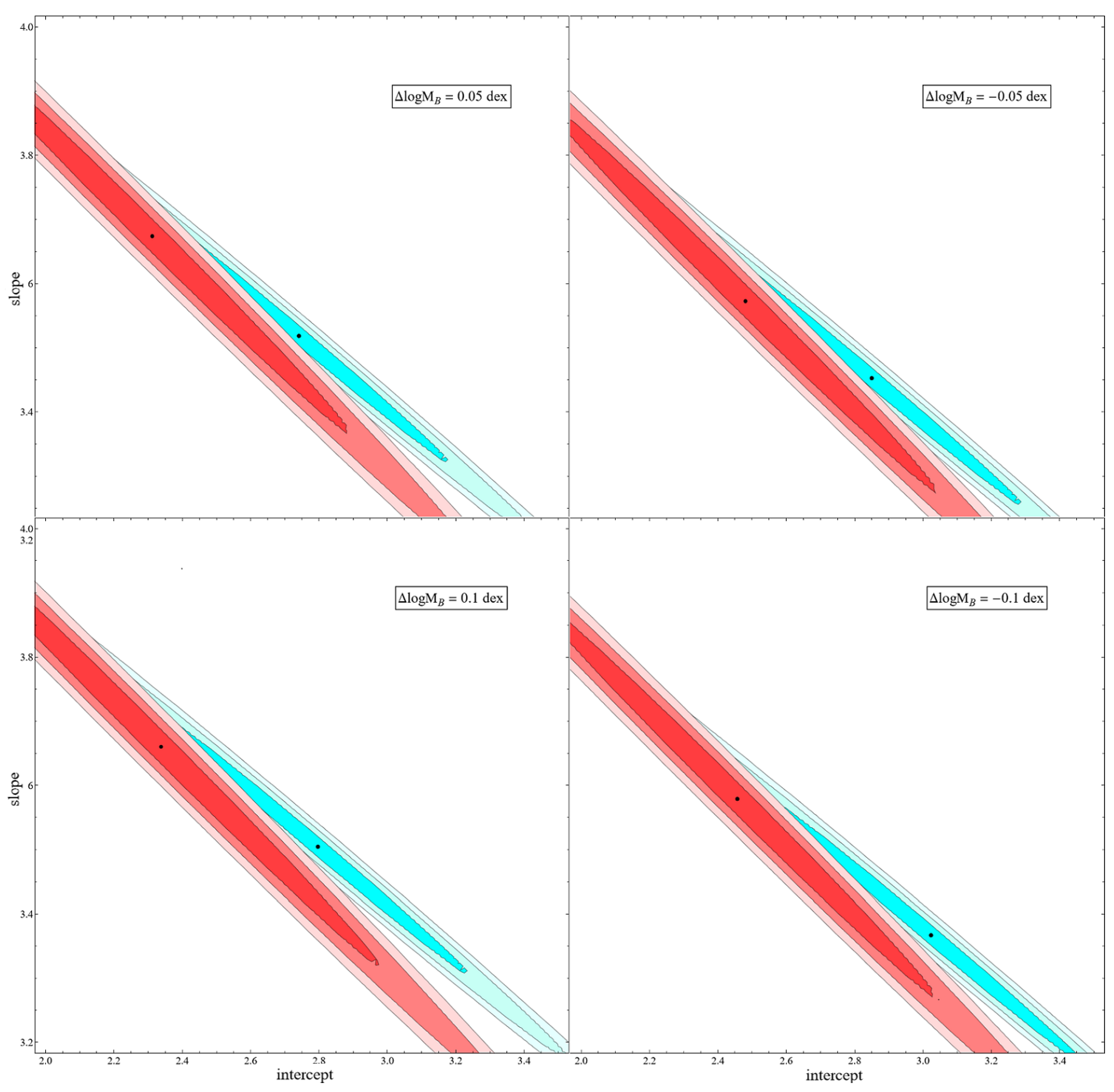
2. Search for Transitions in the Evolution of the BTFR

The logarithmic form of the BTFR (Equation (2)) is as follows:
y = l o g M B = s l o g v r o t + l o g A B s x + b
and a similar form for the TFR. Due to Equation (4), the intercept b l o g A B depends on both the galaxy formation mechanisms through the surface density S and on the strength of gravitational interactions through G eff .
A controversial issue in the literature is the type of possible evolution of the slope and intercept of the TFR and the BTFR. Most studies have searched for possible evolution in high redshifts (redshift range z [ 0 , 3 ] ) with controversial results. For example, several studies found no statistically significant evolution of the intercept of the TFR up to redshifts of z 1.7 [52,53,54,55,56,57,58], while other studies found a negative evolution of the intercept up to redshift z 3   [59,60,61,62,63,64,65,66]. Similar controversial results in high z appeared for the BTFR, where [60] found no significant evolution of the intercept since z 0.6 , while [64] found a positive evolution of the intercept between low-z galaxies and a z 2 sample. In addition, cosmological simulations of disc galaxy formation based on cosmological N-body/hydrodynamical simulations have indicated no evolution of the TFR based on stellar masses in the range z [ 0.1 ] [67], indicating also that any observed evolution of the TFR is an artifact of the luminosity evolution.
These studies have focused mainly on comparing high-z with low-z samples, making no attempt to scan low redshift samples for abrupt transitions of the intercept and slope. Such transitions would be hard to explain in the context of known galaxy formation mechanisms but are well motivated in the context of fundamental gravitational constant transitions, which may be used to address the Hubble tension [22,23]. Thus, in this section, we attempt to fill this gap in the literature.
We consider the BTFR dataset shown in Appendix A based on the data from [12,31,32,33] of the flat rotation velocity of galaxies vs. the baryonic mass (stars plus gas) consisting of 118 datapoints, shown in Table A1. The sample is restricted to those objects for which both quantities are measured to better than 20 % accuracy and includes galaxies in the approximate distance range D [ 1 , 130 ] Mpc . This is a robust low z dataset ( z < 0.1 ) with low scatter showing no evolution of velocity residuals as a function of the central surface density of the stellar disks.
Our analysis is distinct from previous studies in two aspects:
  • We use an exclusively low z sample to search for BTFR evolution.
  • We focus on a particular type of evolution: sharp transitions of the intercept and slope.
In this context, we use the dataset shown in Table A1 of Appendix A [12,31,32,33], consisting of the distance D, the logarithm of the baryonic mass l o g M B and the logarithm of the asymptotically flat rotation velocity l o g v r o t of 118 galaxies along with 1 σ errors. We fix a critical distance D c and split this sample in two subsamples Σ 1 (galaxies with D < D c ) and Σ 2 (galaxies with D > D c ). For each subsample, we use the maximum likelihood method [68] and perform a linear fit to the data setting y i = l o g ( M B ) i , x i = l o g ( v r o t ) i , while the parameters to fit are the slope s and the intercept b of Equation (7). Thus, for each sample j ( j = 0 , 1 , 2 with j = 0 corresponding to the full sample and j = 1 , 2 corresponding to the two subsamples Σ 1 and Σ 2 ), we minimize the following:
χ j 2 ( s , b ) = i = 1 N j y i ( s j x i + b j ) 2 s j 2 σ x i 2 + σ y i 2 + σ s 2
with respect to the slope s j and intercept b j . We fix the scatter to σ s = 0.077 , obtained by demanding that χ 0 , m i n 2 N 0 = 1 , where χ 0 , m i n 2 is the minimized value of χ 2 for the full sample and N 0 is the number of datapoints of the full sample. We thus find the best fit values of the parameters s j and b j , ( j = 0 , 1 , 2 ) and also construct the 1 σ 3 σ likelihood contours in the s b parameter space for each sample (full, Σ 1 and Σ 2 ) for a given value of D c . We then evaluate the Δ χ k l 2 ( D c ) of the best fit of each subsample k, best fit with respect to the likelihood contours of the other subsample l. Using these values, we also evaluate the σ -distances ( d σ , k l ( D c ) and d σ , l k ( D c ) ) and conservatively define the minimum of these σ -distances as follows:
d σ ( D c ) M i n d σ , 12 ( D c ) , d σ , 21 ( D c )
For example, for the σ -distance of the best fit of Σ 1 with respect to the likelihood contours of Σ 2 , we have the following:
Δ χ 12 2 ( D c ) χ 2 2 ( s 1 , b 1 ) ( D c ) χ 2 , m i n 2 ( s 2 , b 2 ) ( D c )
and d σ , 12 is obtained as a solution of the following equation [68]:
Δ χ 12 2 = 2 Q 1 M 2 , 1 Erf ( d σ , 12 2 )
where Q 1 is the inverse regularized incomplete Gamma function, M is the number of parameters to fit ( M = 2 in our case) and Erf is the error function.
Figure 1 shows the σ distance d σ ( D c ) in the parameter space ( b , s ) as a function of the split sample distance D c . There are two peaks indicating larger than 3 σ difference between the two subsamples at D c = 9 Mpc and D c = 17 Mpc. In addition, a transition of the σ distance d σ ( D c ) at D c 20 Mpc is apparent. This Monte Carlo simulation is used to construct Figure 2 (right panel—green line—range), where we show the mean and standard deviation range of the σ -distances obtained by the above-described 100 Monte Carlo samples. Clearly, the random variation in the galactic distances cannot change the qualitative features (high double peak at low D c ) of Figure 1 corresponding to the real sample. The σ -distances obtained from such a typical Monte Carlo sample is shown in Figure 2 (left panel green line).
The typical qualitative feature of d σ ( D c ) corresponding to the real sample disappears if we homogenize the sample by randomizing both the velocities and the galactic masses, using the measured values of the velocities and the estimated values of the galactic masses in the context of the best-fit BTFR. In order to construct such a homogenized BTFR sample from the real sample, we use the following steps:
  • We assign to each galaxy a randomly chosen distance obtained from a Gaussian distribution with mean equal to the measured distance and standard deviation equal to the 1 σ error of the measured distance.
  • We assign to each galaxy a randomly chosen l o g v r o t obtained from a Gaussian distribution with mean equal to the measured l o g v r o t and standard deviation equal to the 1 σ error of the measured l o g v r o t .
  • For each galaxy, we use the random l o g v r o t obtained in the previous step to calculate the corresponding BTFR l o g M B , using the best-fit slope and intercept of the real full dataset (first row of Table 2). We then obtain a random l o g M B for each galaxy from a Gaussian distribution with mean equal to the BTFR calculated l o g M B and standard deviation equal to the 1 σ error of the measured l o g M B .
  • We repeat the above process 100 times, thereby generating 100 homogeneous Monte Carlo samples (HMCS) based on the SPARC dataset.
  • For each HMCS, we find the σ distances d σ ( D c ) and for each D c , we find the mean σ distance and its standard deviation over the 100 HMCS. We thus construct the orange region in Figure 2 (right panel). A typical form of d σ ( D c ) is shown as the orange line of Figure 2 (left panel) selected from the 100 HMCS.
Clearly, the forms of d σ ( D c ) generated from the homogenized Monte Carlo samples have the expected property to be confined mainly between 0 σ and 2 σ in contrast to the real measured sample, where d σ ( D c ) extends up to 4 σ or more. Thus, the real dataset is statistically distinct from a homogeneous BTFR dataset.
The two maxima of d σ are more clearly illustrated in Figure 3, where the likelihood contours are shown in the parameter space s (slope)-b (intercept) for the full sample (upper left panel) and for three pairs of subsamples Σ i , including those corresponding to the peaks shown in Figure 1 ( D c = 17 and D c = 9 ). For both d σ maxima, the tension between the two best-fit points is mainly due to the different intercepts, while the values of the slope are very similar for the two subsamples. In contrast, for D c = 40 Mpc , where the σ distance is much lower (about 1 σ , lower right panel), both the slope and the intercept differ significantly in magnitude but the statistical significance of this difference is low. Notice that the use of different statistics, such as the 1 σ range of the best-fit intercept and slope shown in Table 2, or the level of likelihood contour overlap in Figure 3 would not reveal the tension between far and nearby subsamples. In contrast, the σ -distance statistic demonstrates the effect and the Monte Carlo results of Figure 2 verify the fact that such a large σ -distance would be rare in the context of a homogeneous sample.
The statistical significance of the different Tully–Fisher properties between near and far galaxies, which abruptly disappears for dividing distance D c 20 Mpc, could be an unlikely statistical fluctuation, a hint for systematics in the Tully–Fisher data1, an indication for an abrupt change in the galaxy evolution or a hint for a transition in the values of fundamental constants and, in particular, the strength of gravitational interactions G eff . The best-fit values of the intercept and the slope for the cases shown in Figure 3 are displayed in Table 2 along with their 1 σ errors.
The best-fit l o g M B l o g v r o t lines corresponding to Equation (7) for the near–far galactic subsamples are shown in Figure 4, superimposed with the datapoints (red/blue correspond to near/far galaxies). The full dataset corresponds to the upper-left panel. The difference between the two lines for D c = 9 Mpc and D c = 17 Mpc is evident, even though their slopes are very similar. The statistical significance of this difference disappears for larger values of the splitting distance (e.g., D c = 40 Mpc ), even though the slopes of the two lines become significantly different in this case.
The Hubble diagram of the considered dataset along with the best-fit line (black dot-dashed line) and the Hubble blue dashed line ( z D c H 0 ) corresponding to H 0 = 73 km s 1 Mpc 1 is shown in Figure 5. The distances to galaxies beyond 20 Mpc are determined using the Hubble flow with H 0 = 73 km/sec Mpc, and thus, there is no effect of their peculiar velocities. Galaxies closer than about D 20 Mpc are clearly not in the Hubble flow and their redshift is affected significantly by their in-falling peculiar velocities, which tend to reduce their cosmological redshifts. The detected transitions at about 9 Mpc and 17 Mpc correspond to cosmological redshifts of z 0.005 , which is lower than the transition redshift required for the resolution of the Hubble tension ( z t 0.07 is the upper redshift of SnIa–Cepheid host galaxies).
In the context of the above-described analysis, we have ignored the possible systematic uncertainties induced on the estimated baryonic masses M B , due to systematic uncertainties in the measurement of galactic distances. In particular, different sub-samples of galaxies in the SPARC database are affected by different systematic uncertainties. The SPARC sample includes galaxies with both direct and indirect distance measurements. Direct distance measurements are based on standard candles (Cepheids and Tip of Red Giant stars), while indirect measurements are based on the Hubble flow with Virgocentric infall correction. Systematic uncertainties of indirectly measured distances affecting mainly galaxies beyond 15 Mpc are due to uncertainties in the Hubble constant H 0 and in the a Virgocentric infall model. H 0 = 73 km / s / Mpc is assumed in estimating the distances of the Hubble flow subsample of the SPARC sample along with the Virgocentric infall model used to correct the Hubble flow distances. The anticipated shift in l o g M B due to an incorrect assumption of the H 0 value and/or the Virgocentric infall model is anticipated to be of the order of 0.1 dex, assuming a 5 % change in H 0 and a scaling of the estimated value of M B with distance D as M B D 2 .
Thus, the identified mismatch of the Tully–Fisher parameters between low- and high-distance subsamples could, in principle, be due to such a systematic uncertainty of the galactic baryonic masses of Hubble flow galaxies. In order to examine this possibility, we have constructed new Monte Carlo samples where we not only vary randomly the distances but also add a fixed shift of Δ l o g M B along the vertical axis (mass) for all the datapoints where the mass is estimated using the Hubble flow with H 0 = 73 km / s / Mpc . The distances of these points are calculated using the Hubble flow, assuming H 0 = 73 km s 1 Mpc 1 , and correcting for Virgo-centric infall. We have considered four cases of systematic shifts (fixed values of Δ l o g M B ): 0.1 dex, 0.05 dex, + 0.05 dex and + 0.1 dex. The results for the σ -distance ranges in terms of the splitting distance D c for each one of the above four cases are shown in Figure 6. The corresponding likelihood contours for the subsamples corresponding to D c = 9 Mpc (maximum mismatch) are shown in Figure 7. Clearly, the mismatch features at D c = 9 Mpc and D c = 17 Mpc remain in all four cases that explore this type of systematic uncertainty. In particular, the 9 Mpc peak height varies from about 4 σ for Δ l o g M B = 0.1 dex to about 3 σ for Δ l o g M B = 0.1 dex. We thus conclude that this type of systematic uncertainty is unable to wash out the mismatch effect we have identified.
If the intercepts’ transitions are interpreted as being due to a transition in G eff , we can use Equation (4) along with the observed intercept transition amplitude shown in Table 2 to identify the magnitude and sign of the corresponding G eff transition. The intercept transition at D c = 17 Mpc indicated in Table 2 corresponds to the following:
Δ l o g A B l o g A B > l o g A B < 0.2
Since A B is found to be higher at larger distances (early times), G eff should be lower, due to Equation (4). The corresponding fractional change in G eff is easily obtained by differentiating the logarithmic form of Equation (4) as follows:
Δ l o g A B = Δ A B A B = 2 Δ G eff G eff Δ G eff G eff 0.1
This sign (weaker gravity at early times) and magnitude of the G eff transition is consistent with the gravitational transition required for the resolution of the Hubble and growth tensions in the context of the mechanism of Ref. [22].

3. Conclusions-Discussion

We used a specific statistic on a robust dataset of 118 Tully–Fisher datapoints to demonstrate the existence of evidence for a transition in the evolution of BTFR. This evidence was verified by a wide range of Monte Carlo simulations that compare the real dataset with corresponding homogenized datasets constructed using the BTFR. It indicates a transition of the best-fit values of BTFR parameters, which is small in magnitude but appears at a level of statistical significance of more than 3 σ . It corresponds to a transition of the intercept of the BTFR at a distance of D c 9 Mpc and/or at D c 17 Mpc (about 80 million years ago or less). Such a transition could be interpreted as a systematic effect or as a transition of the effective Newton constant with a 10 % lower value at early times, with the transition taking place about 80 million years ago or less. The amplitude and sign of the gravitational transition are consistent with a recently proposed mechanism for the resolution of the Hubble and growth tensions [22,23]. However, the time of the transition is about 60 million years later than the time suggested by the above mechanism (100–150 million years ago corresponding to D c 30–40 Mpc and z 0.007–0.01).
The effect shown in our analysis could be attributed to causes other than a gravitational transition. One such possible cause would be the presence of systematic errors affecting the estimate of galactic masses or rotation velocities for particular distance ranges. Even if this is the case, it is important to point out these inhomogeneities, which may require further analysis to identify their origin. Alternatively, if the causes of the detected mismatch are physical, they could also be due to variation of conventional galaxy formation mechanisms, which may involve other types of modifications of gravitational physics (e.g., effects of MOND gravity). The BTFR is an observationally tight empirical correlation and has therefore been used as a test of various modified gravity models (Refs. [71,72,73] offer comprehensive reviews on the cosmological implications of such models), including modified Newtonian dynamics (MOND) [74,75] and Grumiller modified gravity [76].These models have been shown to be consistent with BTFR for specific values of their acceleration parameters. The BTFR has also been used as a test of the properties of Cold Dark Matter and galaxy formation mechanisms in the context of Λ CDM [77,78].
An interesting effect in the direction of the one observed in our analysis was also reported in Ref. [79]. There, the authors found a transition of the Cepheid magnitude behavior in the range of 10–20 Mpc, which could explain the Hubble tension (see Figure 4 of Ref. [79]). The authors claimed that this transition is probably due to dust property variation, but there is currently a debate on the actual cause of this mismatch.
An important extension of this analysis is the search for similar transition signals and constraints in other types of astrophysical and geophysical–climatological data of Earth paleontology. For example, a wide range of solar system anomalies were discussed in Ref. [80], which could be revisited in the context of the gravitational transition hypothesis. Of particular interest, for example, is the ‘Faint young Sun paradox’ [81], which involves an inconsistency between geological findings and solar models about the temperature of the Earth about 4 billion years ago. Another interesting extension of this study would be the use of alternative methods for the identification of transition-like features in the data, e.g., the use of a Bayesian analysis tool, such as the internal robustness described in Refs. [82,83].
Alternatively, other astrophysical relations that involve gravitational physics, such as the Faber–Jackson relation between intrinsic luminosity and velocity dispersion of elliptical galaxies or the Cepheid star period–luminosity relation, could also be screened for similar types of transitions as in the case of BTFR. For example, the question to address in the Cepheid case would be the following: ‘What constraints can be imposed on a transition-type evolution of the absolute magnitude ( M v )-period (P) relation of Population I Cepheid stars?’ This relation may be written as follows:
M v = s ( l o g P 1 ) + b
where s = 2.43 ± 0.12 and b = 4.05 ± 0.02 [84,85].
In conclusion, the low z gravitational transition hypothesis is weakly constrained in the context of current studies but it could lead to the resolution of important cosmological tensions of the standard Λ CDM model. We have demonstrated the existence of hints for such a transition in the evolution of the Tully–Fisher relation.

Author Contributions

L.P. contributed in the conceptualization, the methodology, the writing, as well as the general supervision of the project. G.A. contributed in the formal data analysis and the writing. I.A. contributed in the data curation and the literature investigation. All authors have read and agreed to the published version of the manuscript.

Funding

The research of LP and GA is co-financed by Greece and the European Union (European Social Fund—ESF) through the Operational Program “Human Resources Development, Education and Lifelong Learning 2014-2020” in the context of the project MIS 5047648.

Data Availability Statement

The numerical files for the reproduction of the figures can be found in the Tully_Fisher_Transition Github repository under the MIT license (Accessed date: 22 September 2021).

Acknowledgments

We thank Savvas Nesseris and Valerio Marra for their useful comments and suggestions. This research has made use of the SIMBAD database [86], operated at CDS, Strasbourg, France.

Conflicts of Interest

The authors declare no conflict of interest.

Appendix A. Dataset of Galaxies Used

The following is the robust dataset of galaxies used in the analysis. We have used a compilation of 118 datapoints from Refs. [12,31,32,33], for which M B ,   v r o t and D were available.
Table A1. The robust compilation of galaxy data found in Refs. [12,31,32,33].
Galaxy Name Logv rot σ Log v rot LogM B σ Log M B D σ D
(km/s)(km/s)( M )( M )(Mpc)(Mpc)
D631-71.760.038.680.057.720.39
DDO1541.670.028.590.064.040.2
DDO1611.820.039.320.267.52.25
DDO1681.730.038.810.064.250.21
DDO1701.780.039.10.2615.44.62
ESO079-G0142.240.0110.480.2428.77.17
ESO116-G0122.040.029.550.2713.3.9
ESO563-G0212.50.0211.270.1660.89.1
F568-V12.050.119.720.180.68.06
F571-82.150.029.870.1953.310.7
F574-11.990.049.90.196.89.68
F583-11.930.049.520.2235.48.85
IC25741.820.049.280.063.910.2
IC42022.380.0211.030.13100.410.
KK98-2511.530.038.290.266.82.04
NGC00242.030.049.450.097.30.36
NGC00551.930.039.640.082.110.11
NGC01001.940.049.630.2718.450.2
NGC02472.020.049.780.083.70.19
NGC02892.210.0510.860.2220.85.2
NGC03001.970.099.430.082.080.1
NGC08012.340.0111.270.1380.78.07
NGC08912.330.0110.880.119.910.5
NGC10032.040.0210.050.2611.43.42
NGC10902.220.0210.680.2337.9.25
NGC24032.120.029.970.083.160.16
NGC26832.190.0310.620.119.810.49
NGC28412.450.0211.030.1314.11.4
NGC29032.270.0210.650.286.61.98
NGC29151.920.049.0.064.060.2
NGC29761.930.059.280.113.580.18
NGC29982.320.0211.030.1568.110.2
NGC31091.820.038.860.061.330.07
NGC31982.180.0110.530.1113.81.4
NGC35212.330.0310.680.287.72.3
NGC37262.230.0310.640.1518.2.5
NGC37411.70.038.410.063.210.17
NGC37692.070.0410.220.1418.2.5
NGC38772.230.0210.580.1618.2.5
NGC38932.250.0410.570.1518.2.5
NGC39172.130.0210.130.1518.2.5
NGC39492.210.0410.370.1518.2.5
NGC39532.340.0210.870.1618.2.5
NGC39722.120.029.940.1518.2.5
NGC39922.380.0211.130.1323.72.3
NGC40102.10.0210.090.1418.2.5
NGC40132.240.0210.640.1618.2.5
NGC40512.20.0310.710.1618.2.5
NGC40852.120.0210.10.1518.2.5
NGC40882.240.0210.810.1518.2.5
NGC41002.20.0210.530.1518.2.5
NGC41382.170.0510.380.1618.2.5
NGC41572.270.0210.80.1518.2.5
NGC41832.040.0310.0.1418.2.5
NGC42172.260.0210.660.1618.2.5
NGC45592.080.0210.240.277.310.2
NGC50052.420.0410.960.1316.91.5
NGC50332.290.0110.850.2715.74.7
NGC50552.260.0310.960.19.90.5
NGC53712.320.0211.270.2439.79.92
NGC55851.960.029.570.277.062.12
NGC59072.330.0111.060.117.30.9
NGC59852.470.0211.080.2450.350.2
NGC60152.190.0210.380.2717.5.1
NGC61952.400.0311.350.13127.812.8
NGC65032.070.019.940.096.260.31
NGC66742.380.0311.180.1951.210.2
NGC69462.200.0410.610.285.521.66
NGC73312.380.0111.150.1314.71.5
NGC78142.340.0110.590.1114.40.72
UGC001282.120.0510.20.1464.59.7
UGC007311.870.029.410.2612.53.75
UGC012811.750.038.750.065.270.1
UGC022591.940.039.180.2610.53.1
UGC024872.520.0511.430.1669.110.4
UGC028852.460.0211.410.1280.68.06
UGC029162.260.0410.970.1565.49.8
UGC029532.420.0311.150.2816.54.95
UGC032052.340.0210.840.250.10.
UGC035462.290.0310.730.2428.77.2
UGC035802.100.0210.090.2320.75.2
UGC042781.960.039.330.2612.590.2
UGC043251.960.039.280.279.62.88
UGC044991.860.039.350.2612.53.75
UGC052532.330.0411.030.2322.95.72
UGC057161.870.069.240.2221.35.3
UGC057211.90.049.010.266.181.85
UGC059862.050.029.770.278.632.59
UGC063991.930.039.310.1418.2.5
UGC064461.920.049.370.2612.3.6
UGC066142.30.1110.960.1288.78.87
UGC066671.920.029.250.1318.2.5
UGC067862.340.0210.640.2429.37.32
UGC067872.40.0110.750.2421.35.32
UGC068181.850.049.350.1318.2.5
UGC069172.040.039.790.1418.2.5
UGC069231.900.039.40.1418.2.5
UGC069302.030.079.940.1318.2.5
UGC069832.040.039.820.1318.2.5
UGC071251.810.039.880.2619.85.9
UGC071511.870.029.290.086.870.34
UGC073992.010.039.20.278.432.53
UGC075241.90.039.550.064.740.24
UGC076031.790.028.730.264.71.41
UGC076901.760.068.980.278.112.43
UGC082861.920.019.170.066.50.33
UGC084901.90.039.170.114.650.53
UGC085501.760.028.720.266.72.
UGC086992.260.0310.480.2439.39.82
UGC090372.180.0410.780.1183.68.4
UGC091332.360.0411.270.1957.111.4
UGC103101.850.089.390.2715.24.6
UGC114552.430.0111.310.1678.611.8
UGC119142.460.0710.880.2816.95.1
UGC125062.370.0311.070.11100.610.1
UGC126321.860.039.470.269.772.93
UGCA4421.750.038.620.064.350.22
UGCA4441.570.077.980.060.980.05

Note

1
A possible source of systematics is the Malmquist bias, which would imply that the detected more distant galaxies are also more massive and may, therefore, display different slopes and intercepts in different mass bins [69,70].

References

  1. Tully, R.B.; Fisher, J.R. A New method of determining distances to galaxies. Astron. Astrophys. 1977, 54, 661–673. [Google Scholar]
  2. Den Heijer, M.; Oosterloo, T.A.; Serra, P.; Józsa, G.I.G.; Kerp, J.; Morganti, R.; Cappellari, M.; Davis, T.A.; Duc, P.-A.; Emsellem, E.; et al. The Hully-Fisher relation of early-type galaxies. Astron. Astrophys. 2015, 581, A98. [Google Scholar] [CrossRef]
  3. McGaugh, S.S. The Baryonic Tully-Fisher Relation of Galaxies with Extended Rotation Curves and the Stellar Mass of Rotating Galaxies. Astrophys. J. 2005, 632, 859–871. [Google Scholar] [CrossRef] [Green Version]
  4. Aaronson, M.; Huchra, J.; Mould, J. The infrared luminosity/H I velocity-width relation and its application to the distance scale. Astroph. J. 1979, 229, 1–13. [Google Scholar] [CrossRef]
  5. Freeman, K.C. On the Disks of Spiral and S0 Galaxies. Astroph. J. 1970, 160, 811. [Google Scholar] [CrossRef]
  6. Zwaan, M.A.; van der Hulst, J.M.; de Blok, W.J.G.; McGaugh, S.S. The Tully-Fisher relation for low surface brightness galaxies—Implications for galaxy evolution. Mon. Not. R. Astron. Soc. 1995, 273, L35. [Google Scholar] [CrossRef] [Green Version]
  7. McGaugh, S.S.; de Blok, W.J.G. Testing the dark matter hypothesis with low surface brightness galaxies and other evidence. Astrophys. J. 1998, 499, 41. [Google Scholar] [CrossRef] [Green Version]
  8. Dutton, A.A. The baryonic Tully–Fisher relation and galactic outflows. Mon. Not. R. Astron. Soc. 2012, 424, 3123–3128. [Google Scholar] [CrossRef] [Green Version]
  9. Sales, L.V.; Navarro, J.F.; Oman, K.; Fattahi, A.; Ferrero, I.; Abadi, M.; Bower, R.; Crain, R.A.; Frenk, C.S.; Sawala, T.; et al. The low-mass end of the baryonic Tully–Fisher relation. Mon. Not. R. Astron. Soc. 2016, 464, 2419–2428. [Google Scholar] [CrossRef]
  10. Freeman, K.C. On the Origin of the Hubble Sequence. Astrophys. Space Sci. 1999, 269, 119–137. [Google Scholar] [CrossRef]
  11. McGaugh, S.S.; Schombert, J.M.; Bothun, G.D.; de Blok, W.J.G. The Baryonic Tully-Fisher Relation. Astrophys. J. Lett. 2000, 533, L99–L102. [Google Scholar] [CrossRef] [Green Version]
  12. Verheijen, M.A.W. The Ursa Major Cluster of Galaxies. V. H I Rotation Curve Shapes and the Tully-Fisher Relations. Astroph. J. 2001, 563, 694–715. [Google Scholar] [CrossRef]
  13. Zaritsky, D.; Courtois, H.; Munoz-Mateos, J.C.; Sorce, J.; Erroz-Ferrer, S.; Comerón, S.; Gadotti, D.A.; Gil de Paz, A.; Hinz, J.L.; Laurikainen, E. The Baryonic Tully-Fisher Relationship for S4G Galaxies and the ”Condensed” Baryon Fraction of Galaxies. Astron. J. 2014, 147, 134. [Google Scholar] [CrossRef] [Green Version]
  14. Schombert, J.; McGaugh, S.; Lelli, F. Using the Baryonic Tully–Fisher Relation to Measure Ho. Astron. J. 2020, 160, 71. [Google Scholar] [CrossRef]
  15. Riess, A.G.; Casertano, S.; Yuan, W.; Bowers, J.B.; Macri, L.; Zinn, J.C.; Scolnic, D. Cosmic Distances Calibrated to 1% Precision with Gaia EDR3 Parallaxes and Hubble Space Telescope Photometry of 75 Milky Way Cepheids Confirm Tension with ΛCDM. Astrophys. J. Lett. 2021, 908, L6. [Google Scholar] [CrossRef]
  16. Aghanim, N.; Akrami, Y.; Ashdown, M.; Aumont, J.; Baccigalupi, C.; Ballardini, M.; Banday, A.J.; Barreiro, R.B.; Bartolo, N.; Basak, S.; et al. Planck 2018 results. VI. Cosmological parameters. Astron. Astrophys. 2020, 641, A6. [Google Scholar] [CrossRef] [Green Version]
  17. Perivolaropoulos, L.; Skara, F. Challenges for ΛCDM: An update. arXiv 2021, arXiv:2105.05208. [Google Scholar]
  18. Di Valentino, E.; Mena, O.; Pan, S.; Visinelli, L.; Yang, W.; Melchiorri, A.; Mota, D.F.; Riess, A.G.; Silk, J. In the Realm of the Hubble tension—A Review of Solutions. arXiv 2021, arXiv:2103.01183. [Google Scholar]
  19. Kazantzidis, L.; Perivolaropoulos, L. Is gravity getting weaker at low z? Observational evidence and theoretical implications. arXiv 2019, arXiv:1907.03176. [Google Scholar]
  20. Alestas, G.; Kazantzidis, L.; Perivolaropoulos, L. H0 tension, phantom dark energy, and cosmological parameter degeneracies. Phys. Rev. D 2020, 101, 123516. [Google Scholar] [CrossRef]
  21. Alestas, G.; Perivolaropoulos, L. Late-time approaches to the Hubble tension deforming H(z), worsen the growth tension. Mon. Not. R. Astron. Soc. 2021, 504, 3956–3962. [Google Scholar] [CrossRef]
  22. Marra, V.; Perivolaropoulos, L. A rapid transition of Geff at zt≃0.01 as a solution of the Hubble and growth tensions. arXiv 2021, arXiv:2102.06012. [Google Scholar]
  23. Alestas, G.; Kazantzidis, L.; Perivolaropoulos, L. A w-M phantom transition at zt<0.1 as a resolution of the Hubble tension. arXiv 2020, arXiv:2012.13932. [Google Scholar]
  24. Camarena, D.; Marra, V. A new method to build the (inverse) distance ladder. Mon. Not. R. Astron. Soc. 2020, 495, 2630–2644. [Google Scholar] [CrossRef]
  25. Amendola, L.; Corasaniti, P.S.; Occhionero, F. Time variability of the gravitational constant and type Ia supernovae. arXiv 1999, arXiv:astro-ph/9907222. [Google Scholar]
  26. Gaztanaga, E.; Garcia-Berro, E.; Isern, J.; Bravo, E.; Dominguez, I. Bounds on the possible evolution of the gravitational constant from cosmological type Ia supernovae. Phys. Rev. D 2002, 65, 023506. [Google Scholar] [CrossRef] [Green Version]
  27. Wright, B.S.; Li, B. Type Ia supernovae, standardizable candles, and gravity. Phys. Rev. D 2018, 97, 083505. [Google Scholar] [CrossRef] [Green Version]
  28. Übler, H.; Förster Schreiber, N.M.; Genzel, R.; Wisnioski, E.; Wuyts, S.; Lang, P.; Naab, T.; Burkert, A.; van Dokkum, P.G.; Tacconi, L.J.; et al. The Evolution of the Tully-Fisher Relation between z ~ 2.3 and z ~ 0.9 with KMOS3D. Astroph. J. 2017, 842, 121. [Google Scholar] [CrossRef]
  29. Esposito-Farese, G.; Polarski, D. Scalar tensor gravity in an accelerating universe. Phys. Rev. D 2001, 63, 063504. [Google Scholar] [CrossRef] [Green Version]
  30. Alvey, J.; Sabti, N.; Escudero, M.; Fairbairn, M. Improved BBN Constraints on the Variation of the Gravitational Constant. Eur. Phys. J. C 2020, 80, 148. [Google Scholar] [CrossRef]
  31. Walter, F.; Brinks, E.; de Blok, W.J.G.; Bigiel, F.; Kennicutt, R.C.; Thornley, M.D.; Leroy, A. Things: The H I nearby galaxy survey. Astron. J. 2008, 136, 2563–2647. [Google Scholar] [CrossRef]
  32. Lelli, F.; McGaugh, S.S.; Schombert, J.M.; Desmond, H.; Katz, H. The baryonic Tully-Fisher relation for different velocity definitions and implications for galaxy angular momentum. Mon. Not. R. Astron. Soc. 2019, 484, 3267–3278. [Google Scholar] [CrossRef]
  33. Lelli, F.; McGaugh, S.S.; Schombert, J.M. The Small Scatter of the Baryonic Tully-Fisher Relation. Astroph. J. Lett. 2016, 816, L14. [Google Scholar] [CrossRef]
  34. Hofmann, F.; Müller, J. Relativistic tests with lunar laser ranging. Class. Quant. Grav. 2018, 35, 035015. [Google Scholar] [CrossRef]
  35. Pitjeva, E.V.; Pitjev, N.P.; Pavlov, D.A.; Turygin, C.C. Estimates of the change rate of solar mass and gravitational constant based on the dynamics of the Solar System. Astron. Astrophys. 2021, 647, A141. [Google Scholar] [CrossRef]
  36. Pitjeva, E.V.; Pitjev, N.P. Relativistic effects and dark matter in the Solar system from observations of planets and spacecraft. Mon. Not. R. Astron. Soc. 2013, 432, 3431. [Google Scholar] [CrossRef] [Green Version]
  37. Deller, A.T.; Verbiest, J.P.W.; Tingay, S.J.; Bailes, M. Extremely high precision VLBI astrometry of PSR J0437-4715 and implications for theories of gravity. Astrophys. J. Lett. 2008, 685, L67. [Google Scholar] [CrossRef] [Green Version]
  38. Giani, L.; Frion, E. Testing the Equivalence Principle with Strong Lensing Time Delay Variations. J. Cosmol. Astropart. Phys. 2020, 9, 8. [Google Scholar] [CrossRef]
  39. Zhu, W.W.; Desvignes, G.; Wex, N.; Caballero, R.N.; Champion, D.J.; Demorest, P.B.; Ellis, J.A.; Janssen, G.H.; Kramer, M.; Krieger, A.; et al. Tests of Gravitational Symmetries with Pulsar Binary J1713+0747. Mon. Not. R. Astron. Soc. 2019, 482, 3249–3260. [Google Scholar] [CrossRef] [Green Version]
  40. Genova, A.; Mazarico, E.; Goossens, S.; Lemoine, F.G.; Neumann, G.A.; Smith, D.E.; Zuber, M.T. Solar system expansion and strong equivalence principle as seen by the NASA MESSENGER mission. Nat. Commun. 2018, 9, 289. [Google Scholar] [CrossRef] [Green Version]
  41. Masuda, K.; Suto, Y. Transiting planets as a precision clock to constrain the time variation of the gravitational constant. Publ. Astron. Soc. Jap. 2016, 68, L5. [Google Scholar] [CrossRef] [Green Version]
  42. Gaztañaga, E.; Cabré, A.; Hui, L. Clustering of luminous red galaxies—IV. Baryon acoustic peak in the line-of-sight direction and a direct measurement of H(z). Mon. Not. R. Astron. Soc. 2009, 399, 1663–1680. [Google Scholar] [CrossRef] [Green Version]
  43. Córsico, A.H.; Althaus, L.G.; García-Berro, E.; Romero, A.D. An independent constraint on the secular rate of variation of the gravitational constant from pulsating white dwarfs. J. Cosmol. Astropart. Phys. 2013, 6, 32. [Google Scholar] [CrossRef]
  44. Hellings, R.W.; Adams, P.J.; Anderson, J.D.; Keesey, M.S.; Lau, E.L.; Standish, E.M.; Canuto, V.M.; Goldman, I. Experimental Test of the Variability of G Using Viking Lander Ranging Data. Phys. Rev. Lett. 1983, 51, 1609–1612. [Google Scholar] [CrossRef]
  45. Guenther, D.B.; Krauss, L.M.; Demarque, P. Testing the Constancy of the Gravitational Constant Using Helioseismology. Astrophys. J. 1998, 498, 871–876. [Google Scholar] [CrossRef] [Green Version]
  46. Vijaykumar, A.; Kapadia, S.J.; Ajith, P. Constraints on the time variation of the gravitational constant using gravitational wave observations of binary neutron stars. arXiv 2020, arXiv:2003.12832. [Google Scholar]
  47. Uzan, J.P. The Fundamental Constants and Their Variation: Observational Status and Theoretical Motivations. Rev. Mod. Phys. 2003, 75, 403. [Google Scholar] [CrossRef] [Green Version]
  48. Degl’Innocenti, S.; Fiorentini, G.; Raffelt, G.G.; Ricci, B.; Weiss, A. Time variation of Newton’s constant and the age of globular clusters. Astron. Astrophys. 1996, 312, 345–352. [Google Scholar]
  49. Thorsett, S.E. The Gravitational constant, the Chandrasekhar limit, and neutron star masses. Phys. Rev. Lett. 1996, 77, 1432–1435. [Google Scholar] [CrossRef] [Green Version]
  50. Jofre, P.; Reisenegger, A.; Fernandez, R. Constraining a possible time-variation of the gravitational constant through gravitochemical heating of neutron stars. Phys. Rev. Lett. 2006, 97, 131102. [Google Scholar] [CrossRef] [Green Version]
  51. Wu, F.; Chen, X. Cosmic microwave background with Brans-Dicke gravity II: Constraints with the WMAP and SDSS data. Phys. Rev. D 2010, 82, 083003. [Google Scholar] [CrossRef] [Green Version]
  52. Conselice, C.J.; Bundy, K.; Ellis, R.S.; Brichmann, J.; Vogt, N.P.; Phillips, A.C. Evolution of the near-infrared Tully-Fisher relation: Constraints on the relationship between the stellar and total masses of disk galaxies since z = 1. Astrophys. J. 2005, 628, 160–168. [Google Scholar] [CrossRef] [Green Version]
  53. Kassin, S.A.; Weiner, B.J.; Faber, S.M.; Koo, D.C.; Lotz, J.M.; Diemand, J.; Harker, J.J.; Bundy, K.; Metevier, A.J.; Phillips, A.C.; et al. The Stellar Mass Tully-Fisher Relation to z = 1.2 from AEGIS. Astrophys. J. Lett. 2007, 660, L35–L38. [Google Scholar] [CrossRef] [Green Version]
  54. Miller, S.H.; Bundy, K.; Sullivan, M.; Ellis, R.S.; Treu, T. The Assembly History of Disk Galaxies: I—The Tully-Fisher Relation to z~1.3 from Deep Exposures with DEIMOS. Astrophys. J. 2011, 741, 115. [Google Scholar] [CrossRef] [Green Version]
  55. Contini, T.; Epinat, B.; Bouché, N.; Brinchmann, J.; Boogaard, L.A.; Ventou, E.; Bacon, R.; Richard, J.; Weilbacher, P.M.; Wisotzki, L.; et al. Deep MUSE observations in the HDFS—Morpho-kinematics of distant star-forming galaxies down to 108M. Astron. Astrophys. 2016, 591, A49. [Google Scholar] [CrossRef] [Green Version]
  56. Di Teodoro, E.M.; Fraternali, F.; Miller, S.H. Flat rotation curves and low velocity dispersions in KMOS star-forming galaxies at z ∼ 1. Astron. Astrophys. 2016, 594, A77. [Google Scholar] [CrossRef] [Green Version]
  57. Molina, J.; Ibar, E.; Swinbank, A.M.; Sobral, D.; Best, P.N.; Smail, I.; Escala, A.; Cirasuolo, M. SINFONI-HiZELS: The dynamics, merger rates and metallicity gradients of ’typical’ star-forming galaxies at z = 0.8–2.2. Mon. Not. R. Astron. Soc. 2017, 466, 892–905. [Google Scholar] [CrossRef] [Green Version]
  58. Pelliccia, D.; Tresse, L.; Epinat, B.; Ilbert, O.; Scoville, N.; Amram, P.; Lemaux, B.C.; Zamorani, G. HR-COSMOS: Kinematics of star-forming galaxies at z ∼ 0.9. Astron. Astrophys. 2017, 599, A25. [Google Scholar] [CrossRef] [Green Version]
  59. Puech, M.; Flores, H.; Hammer, F.; Yang, Y.; Neichel, B.; Lehnert, M.; Chemin, L.; Nesvadba, N.; Epinat, B.; Amram, P.; et al. IMAGES- III. The evolution of the near-infrared Tully-Fisher relation over the last 6 Gyr. Astron. Astrophys. 2008, 484, 173–187. [Google Scholar] [CrossRef]
  60. Puech, M.; Hammer, F.; Flores, H.; Delgado-Serrano, R.; Rodrigues, M.; Yang, Y. The baryonic content and Tully-Fisher relation at z ∼ 0.6. Astron. Astrophys. 2010, 510, A68. [Google Scholar] [CrossRef] [Green Version]
  61. Cresci, G.; Hicks, E.K.S.; Genzel, R.; Schreiber, N.M.F.; Davies, R.; Bouché, N.; Buschkamp, P.; Genel, S.; Shapiro, K.; Tacconi, L.; et al. The sins survey: Modeling the dynamics of z ∼ 2 galaxies and the high-z tully–fisher relation. Astrophys. J. 2009, 697, 115. [Google Scholar] [CrossRef] [Green Version]
  62. Gnerucci, A.; Marconi, A.; Cresci, G.; Maiolino, R.; Mannucci, F.; Calura, F.; Cimatti, A.; Cocchia, F.; Grazian, A.; Matteucci, F.; et al. Dynamical properties of AMAZE and LSD galaxies from gas kinematics and the Tully-Fisher relation at z ∼ 3. Astron. Astrophys. 2011, 528, A88. [Google Scholar] [CrossRef] [Green Version]
  63. Swinbank, M.; Sobral, D.; Smail, I.; Geach, J.; Best, P.; McCarthy, I.; Crain, R.; Theuns, T. The Properties of the Star-Forming Interstellar Medium at z = 0.84–2.23 from HiZELS-I: Mapping the Internal Dynamics and Metallicity Gradients in High-Redshift Disk Galaxies. Mon. Not. R. Astron. Soc. 2012, 426, 935. [Google Scholar] [CrossRef] [Green Version]
  64. Price, S.H.; Kriek, M.; Shapley, A.E.; Reddy, N.A.; Freeman, W.R.; Coil, A.L.; de Groot, L.; Shivaei, I.; Siana, B.; Azadi, M.; et al. The mosdef survey: Dynamical and baryonic masses and kinematic structures of star-forming galaxies at 1.4 ≤ z ≤ 2.6. Astrophys. J. 2016, 819, 80. [Google Scholar] [CrossRef] [Green Version]
  65. Tiley, A.L.; Stott, J.P.; Swinbank, A.M.; Bureau, M.; Harrison, C.M.; Bower, R.; Johnson, H.L.; Bunker, A.J.; Jarvis, M.J.; Magdis, G.; et al. The KMOS Redshift One Spectroscopic Survey (KROSS): The Tully–Fisher relation at z ∼ 1. Mon. Not. R. Astron. Soc. 2016, 460, 103–129. [Google Scholar] [CrossRef] [Green Version]
  66. Straatman, C.M.S.; Glazebrook, K.; Kacprzak, G.G.; Labbé, I.; Nanayakkara, T.; Alcorn, L.; Cowley, M.; Kewley, L.J.; Spitler, L.R.; Tran, K.V.H.; et al. ZFIRE: The Evolution of the Stellar Mass Tully–Fisher Relation to Redshift ∼ 2.2. Astrophys. J. 2017, 839, 57. [Google Scholar] [CrossRef]
  67. Portinari, L.; Sommer-Larsen, J. The Tully-Fisher relation and its evolution with redshift in cosmological simulations of disc galaxy formation. Mon. Not. R. Astron. Soc. 2007, 375, 913–924. [Google Scholar] [CrossRef] [Green Version]
  68. Press, W.H.; Teukolsky, S.A.; Vetterling, W.T.; Flannery, B.P. Numerical Recipes 3rd Edition: The Art of Scientific Computing, 3rd ed.; Cambridge University Press: New York, NY, USA, 2007. [Google Scholar]
  69. Dutton, A.A.; Obreja, A.; Wang, L.; Gutcke, T.A.; Buck, T.; Udrescu, S.M.; Frings, J.; Stinson, G.S.; Kang, X.; Macciò, A.V. NIHAO XII: Galactic uniformity in a ΛCDM universe. Mon. Not. R. Astron. Soc. 2017, 467, 4937–4950. [Google Scholar] [CrossRef] [Green Version]
  70. Desmond, H. The scatter, residual correlations and curvature of the sparc baryonic Tully–Fisher relation. Mon. Not. R. Astron. Soc. Lett. 2017, 472, L35–L39. [Google Scholar] [CrossRef] [Green Version]
  71. Nojiri, S.; Odintsov, S.D.; Oikonomou, V.K. Modified Gravity Theories on a Nutshell: Inflation, Bounce and Late-time Evolution. Phys. Rept. 2017, 692, 1–104. [Google Scholar] [CrossRef] [Green Version]
  72. Nojiri, S.; Odintsov, S.D. Unified cosmic history in modified gravity: From F(R) theory to Lorentz non-invariant models. Phys. Rept. 2011, 505, 59–144. [Google Scholar] [CrossRef] [Green Version]
  73. Clifton, T.; Ferreira, P.G.; Padilla, A.; Skordis, C. Modified Gravity and Cosmology. Phys. Rept. 2012, 513, 1–189. [Google Scholar] [CrossRef] [Green Version]
  74. Milgrom, M. A modification of the Newtonian dynamics—Implications for galaxies. Astroph. J. 1983, 270, 371–383. [Google Scholar] [CrossRef]
  75. McGaugh, S.S. The baryonic tully–fisher relation of gas-rich galaxies as a test of ΛCDM and MOND. Astron. J. 2012, 143, 40. [Google Scholar] [CrossRef] [Green Version]
  76. Ghosh, S.; Bhadra, A.; Mukhopadhyay, A.; Sarkar, K. Baryonic Tully–Fisher Test of Grumiller’s Modified Gravity Model. Grav. Cosmol. 2021, 27, 157–162. [Google Scholar] [CrossRef]
  77. Blanton, M.R.; Geha, M.; West, A.A. Testing Cold Dark Matter with the Low-Mass Tully-Fisher Relation. Astroph. J. 2008, 682, 861–873. [Google Scholar] [CrossRef] [Green Version]
  78. Governato, F.; Brook, C.; Mayer, L.; Brooks, A.; Rhee, G.; Wadsley, J.; Jonsson, P.; Willman, B.; Stinson, G.; Quinn, T.; et al. Bulgeless dwarf galaxies and dark matter cores from supernova-driven outflows. Nature 2010, 463, 203–206. [Google Scholar] [CrossRef] [Green Version]
  79. Mortsell, E.; Goobar, A.; Johansson, J.; Dhawan, S. The Hubble Tension Bites the Dust: Sensitivity of the Hubble Constant Determination to Cepheid Color Calibration. arXiv 2021, arXiv:2105.11461. [Google Scholar]
  80. Iorio, L. Gravitational Anomalies in the Solar System? Int. J. Mod. Phys. D 2015, 24, 1530015. [Google Scholar] [CrossRef] [Green Version]
  81. Feulner, G. The faint young Sun problem. Rev. Geophys. 2012, 50, RG2006. [Google Scholar] [CrossRef] [Green Version]
  82. Amendola, L.; Marra, V.; Quartin, M. Internal robustness: Systematic search for systematic bias in SN Ia data. Mon. Not. R. Astron. Soc. 2013, 430, 1867–1879. [Google Scholar] [CrossRef] [Green Version]
  83. Heneka, C.; Marra, V.; Amendola, L. Extensive search for systematic bias in supernova Ia data. Mon. Not. R. Astron. Soc. 2014, 439, 1855–1864. [Google Scholar] [CrossRef] [Green Version]
  84. Benedict, G.F.; McArthur, B.E.; Feast, M.W.; Barnes, T.G.; Harrison, T.E.; Patterson, R.J.; Menzies, J.W.; Bean, J.L.; Freedman, W.L. Hubble Space Telescope Fine Guidance Sensor Parallaxes of Galactic Cepheid Variable Stars: Period-Luminosity Relations. Astron. J. 2007, 133, 1810–1827, Erratum in Astron. J. 2007, 133, 2980. [Google Scholar] [CrossRef] [Green Version]
  85. Benedict, G.F.; McArthur, B.E.; Fredrick, L.W.; Harrison, T.E.; Lee, J.; Slesnick, C.L.; Rhee, J.; Patterson, R.J.; Nelan, E.; Jefferys, W.H.; et al. Astrometry with hubble space telescope: A parallax of the fundamental distance calibrator delta cephei. Astron. J. 2002, 124, 1695–1705. [Google Scholar] [CrossRef]
  86. Wenger, M.; Ochsenbein, F.; Egret, D.; Dubois, P.; Bonnarel, F.; Borde, S.; Genova, F.; Jasniewicz, G.; Laloë, S.; Lesteven, S.; et al. The SIMBAD astronomical database. The CDS reference database for astronomical objects. Astron. Astroph. 2000, 143, 9–22. [Google Scholar] [CrossRef] [Green Version]
Figure 1. The σ -distance between the various Σ 1 and Σ 2 datasets as a function of the split distances D c . There are 2 clear peaks at D c = 9 Mpc and D c = 17 Mpc and a transition seems to have been completed at D c 20 Mpc . The anticipated plot would be a σ -distance that consistently varies in the range up to about 2 σ for all values of D c . The observed peaks indicate either the presence of systematics or the presence of interesting physics.
Universe 07 00366 g001
Figure 2. Left panel: The σ -distances as a function of the split distances D c for a sample dataset with random distance values, normally distributed inside their individual 1 σ range (green line), versus the σ -distances as a function of the split distances D c for a homogeneous Monte Carlo sample constructed using the best-fit BTFR (orange line). Right panel: The 68 % range of the σ -distances versus the split distances D c produced by a Monte Carlo simulation of 100 sample datasets obtained by randomly varying galaxy distance values with a Gaussian probability distribution (green band). Superimposed is the 68 % range of the σ -distances versus the split distances D c obtained from 100 homogeneous Monte Carlo samples constructed using the best-fit BTFR (orange band). Evidently, the characteristic two-peak form of the plot remains practically unchanged, even after the random variation in the distances (green band), whereas no significant tension is present in the case of the homogeneous Monte Carlo samples for any value of D c (orange band).
Universe 07 00366 g002
Figure 3. The best-fit contours of the slope and intercept for the entire dataset, as well for 3 different cases of split distance ( D c ). The red contours correspond to the dataset with galaxies that have a distance below D c , whereas the cyan contours correspond to galaxies with distances above D c .
Universe 07 00366 g003
Figure 4. The best-fit lines corresponding to the best fit slope and intercept parameters of the whole galaxy dataset as well as each of the 2 datasets produced for 4 different split distances ( D c ). The red dashed line and datapoints correspond to the data below D c , and the cyan ones belong to the data over D c for each case.
Universe 07 00366 g004
Figure 5. The distances alongside their errorbars versus the redshifts of each galaxy in our compilation. The blue dashed line corresponds to the best fit line, and the black dot-dashed one is produced by Equation (1) for H 0 = 73 km s 1 Mpc 1 .
Universe 07 00366 g005
Figure 6. The 68 % range of the σ -distances versus the split distances D c produced by a Monte Carlo simulation of 100 sample datasets. The simulations are performed for different values of the shift Δ l o g M B , which represents the possible systematic errors present in the datapoints whose distances are calculated using the Hubble flow, assuming H 0 = 73 km s 1 Mpc 1 , and correcting for Virgo-centric infall. The same characteristic two-peak structure remains for all shifts considered, indicating the robust nature of the identified effect.
Universe 07 00366 g006
Figure 7. The likelihood contours of the slope and intercept for a sample splitting distance D c = 9 Mpc corresponding to the different values of the systematic shift Δ l o g M B shown in Figure 6. The red contours correspond to the dataset with galaxies that have distance below 9 Mpc, whereas the cyan contours correspond to galaxies with distances above 9 Mpc. The σ distance between the two best fits varies between 3 σ and 4 σ .
Universe 07 00366 g007
Table 2. The best-fit values of the intercept and slope parameters corresponding to the likelihood contours of Figure 3 alongside with their 1 σ errors. The minimum Δ χ 2 between the best fits of the two samples is also shown. The corresponding σ -tension in parenthesis is obtained in the context of two free parameters from Equation (11). Notice that, even though the parameter values appear to be consistent, the value of Δ χ 2 between the subsamples reveals the tension at D c = 9 Mpc and D c = 17  Mpc.
D c (Mpc)InterceptSlope Δ χ min 2
- 2.287 ± 0.18 3.7 ± 0.08 -
<9 2.461 ± 0.407 3.586 ± 0.216 23.7 ( 4.5 σ )
>9 2.854 ± 0.379 3.46 ± 0.204 23.7 ( 4.5 σ )
<17 2.467 ± 0.38 3.592 ± 0.17 17.0 ( 3.7 σ )
>17 2.677 ± 0.368 3.548 ± 0.166 17.0 ( 3.7 σ )
<40 2.327 ± 0.987 3.681 ± 0.419 2.9 ( 1.2 σ )
>40 3.318 ± 0.816 3.283 ± 0.349 2.9 ( 1.2 σ )
Publisher’s Note: MDPI stays neutral with regard to jurisdictional claims in published maps and institutional affiliations.

