Abstract
For a scenario of a close flyby of a compact star near a spinning black hole, we provide analytical and numerical estimates for the shift of trajectory periastron due to relativistic (beyond post-Newtonian) effects. More specifically, we derived a generalized expression (not limited to quasi-circular or elliptical orbits) directly linking the periastron shift and the spin of the black hole. The expression permits the estimation of black hole spin based on astronomical tracking of locations of stars traveling along highly eccentric (parabolic and hyperbolic) trajectories in close vicinity of a black hole. We also demonstrate how stars traveling on hyperbolic or parabolic trajectories may be (temporarily) captured onto quasi-circular orbits around black holes, and we quantitatively examine conditions for such scenarios.
1. Introduction
The spin of a black hole (BH) is a critically important parameter in many problems of astrophysics. A number of spin measurement techniques have been developed over the decades, but challenges remain (see, for example, Review [1]). For a while, spin measurements were only possible based on observations of accretion disks. For accreting supermassive black holes in active galactic nuclei, or for accreting stellar mass black holes in X-ray binaries, observations of the accreting gas—its emissions or temperature—can be used to deduce the disk structure affected by the frame-dragging due to BH spin. Indeed, the position of the innermost stable circular orbit (ISCO)—the transition between the Newtonian zone and the zone where relativistic effects become important, destabilizing circular orbits and causing the accreting gas to undergo a plunging spiral into the BH event horizon—is a basic property of the BH gravitational field and depends on the spin. The key challenge is to understand the influence of frame-dragging on accretion disk structure and compare these expectations to data from real black holes. The more recently developed BH spin measurement methods have their challenges as well. Thus, although gravitational waves can provide information about the binary equivalent of the ISCO during the merger of a binary BH system, for single black holes, no systematic gravitational waves are expected. Another method—imaging with the Even Horizon Telescope—can detect the asymmetry in brightness between the approaching and receding sides of the disk, which are strongly spin-dependent. However, interpretation of the data depends on the modeled time and space variability of the accretion disk and the foreground distribution of galactic gas that acts as a varying scattering screen. Finally, observations of stellar orbits in the close vicinity of black holes may also reveal the BH spin. We focus our work on this method.
It is well-known that studies of the differences between the observed stellar trajectories near a black hole and the hypothetical trajectories of the stars estimated within the Newtonian framework help not only to verify the current theory of relativity, but also determine characteristics of the black hole and the orbiting stars (see, for example, refs. [2,3,4,5], and references therein). Obviously, relativistic effects are the strongest in the vicinity of the periastron—the point where the traveling object is the closest to the gravitationally powerful attractor. The closest approaches to the attractor may occur when stellar objects travel along strongly-elongated elliptical orbits or parabolic/hyperbolic trajectories. In close vicinity of a spinning black hole, the commonly used post-Newtonian approximation may become inaccurate. In this paper, we develop analytical and numerical estimates for the shift of the periastron due to relativistic (beyond post-Newtonian) effects.
Specifically, we focus on the following questions: In close vicinity of a spinning black hole, how strong is the periastron shift (relative to its Newtonian proxy)? How many revolutions around the black hole does it take for the test-body to reach the periastron? What parameters determine the revolution-number, and what is the dependence-function? Under what conditions does the body inevitably fall into the ergozone? The questions seem simple, but upon closer examination, the results are not at all obvious. Furthermore, our goal is not only to obtain these estimates, but also to outline the method by which these estimates are obtained. Indeed, in view of the prevalent use of powerful numerical simulations being the main approach to problem solving, a recourse to the concept—a theoretical method is more important than a result, because an error-free method generates additional correct results—seems to be methodically justified. Analyses of the questions listed above must include the premises that the effects of both relativistic theories are strong, the black hole spinning is rapid, and that the effect is studied from the perspective of a distant observer (i.e., located not in a co-moving frame).
The sequence of steps in the analytical approach is the following: (a) we start with articulation of the principle of least action within a specific structure of spacetime in the vicinity of a spinning black hole; (b) we construct the Lagrangian for the test body of finite mass; (c) we find equations of motion for the body; (d) from the symmetry of the Lagrangian, we find the integrals of motion; (e) finally, we obtain the key equation for the trajectory, which captures the nonlinear general-relativistic effects (including the “rotation” of the black hole); (f) we calculate the periastron’s shift and find (for a parabolic trajectory) the conditions under which the body falls onto the static limit—the boundary of ergosphere where the frame-dragging becomes irresistible and all matter and light is forced to rotate around the black hole. To give a consistent presentation of the method for calculating the characteristics of the process, we include a brief overview of the properties of spacetime in the vicinity of a rotating black hole.
The structure of the paper is as follows: In Section 2, the problem is defined. To avoid unnecessary complications in the calculations, we suppose that the traveling object is not destroyed by tidal forces. In Section 3, the motion regime of the compact star moving in the vicinity of the spinning black hole, and the estimate of the periastron shift, are given. The calculated effect opens up (in principle) a new opportunity for the estimation of the rates of rotation of black holes based on observed distortions of trajectories of compact stars traversing their vicinity. Indeed, position-tracking for stars moving along, not quasi-circular but, highly eccentric orbits, or open trajectories, near supermassive stars (black holes), and subsequent quantification of for the descending and outgoing parts of the trajectories, can offer validating arguments for the employed relativistic model. Section 4 concludes with a discussion and final remarks.
2. Model
2.1. Metric near Spinning Black Hole
A non-charged black hole is described by the Kerr metric: an exact, singular, stationary and axially symmetric solution of the Einstein–Hilbert equations of the gravitational “field” in vacuum. It is generally accepted that the spacetime near any massive object M, which possesses angular momentum , may also be described by the Kerr metric [6,7,8,9,10,11,12]. In the Boyer–Lindquist coordinates, the components of the metric tensor can be found from expression
which is given here in dimensional units. Here and further on, we employ the metric signature for the Minkowski tensor, which is also commonly used (see, for example, ref. [13]). The four coordinates represent a world event. They are defined from the viewpoint of a remote observer. The meaning of space coordinates is clear once transitioned to the limit and . When the square of the interval becomes , i.e., at infinity, parameters may be interpreted as the standard spherical coordinates in flat spacetime. Note again that the first term has the plus sign in front of it. Within the used parametrization—Equation (1)—the z-axis and the BH angular momentum are co-aligned. Here also: is the Schwarzschild radius, c is the speed of light, G is the gravitational constant. Equation (1) uses length-scales , , and , for succinctness:
Parameter is a measure of the BH “rate of rotation”. Some publications use notation or notation a. Parameter may be not be negligible in some physically-interesting cases. For the Sun, for example, the angular moment , giving (not negligibly small).
To satisfy the principle of causality for material objects, it must be that . As for the parameter r, note that it is not the “distance” from the black hole. This is because, for any material object, in the spacetime defined by Equation (1), no central point exists in the sense of a world-event on a valid world-line.
Besides the Boyer–Lindquist coordinates, other representations of spacetime locations exist (see, for example, refs. [14,15]).
The cross-product term, , plays a key role in the spacetime metric near spinning black holes. It describes the coupling of time and space. When the angular momentum can be disregarded, the coupling disappears.
In units of length and time , when , , and is replaced with , then
where
From expressions (3) and (4), it is apparent that, in the Kerr metric, there exist hyper-surfaces where components of metric tensor permit certain features. Four such hyper-surfaces exist, but two are “hidden beneath” the event horizon.
One of the surfaces corresponds to the event horizon. At this surface, the value for the purely radial component of the metric goes to infinity. Equation yields two solutions. The physically meaningful one is: . It reveals that parameter is always A quickly-spinning black hole with is a maximally-rotating object. In some works, for example [8], calculations of some effects are carried out even with . Besides the singularity at the event horizon, one more singularity arises when the component of the metric tensor goes to zero. Again, equation (which has two solutions) gives the physically meaningful solution: . Because of underneath the radical sign, this outer hyper-surface (known as the “static limit”) looks like a flattened sphere, which at the poles, where latitude equals 0 or , touches the event horizon.
Between these two hyper-surfaces lies the ergosphere. There—in the chosen Boyer–Lindquist coordinate presentation—the component of the metric tensor is negative, i.e., the time coordinate manifests itself as a spatial coordinate. See Ref. [16] for a discussion on the meaning of singularities within and at the ergozone.
2.2. Equations of Motion
2.2.1. Extremum of Action
The motion of a free test-body in a gravitational field is determined by the same principle of least action as in the special theory of relativity. The gravitational field becomes manifested only via the changed expression for the interval in terms of quantities when .
The action S is determined by the proper time integral between two world-points [17], which can be rewritten as
Here, is a selected affine parameter (such as s, t, or proper time , for example)
Thus, the quantity can be identified as the Lagrangian of the test-body. The extremum of action S is found from setting the variational derivatives to zero
Here, the functional derivative of variables with respect to , is shifted to the left and it is taken into account that the Lagrangian is always determined up to an inessential term which can be omitted. Keeping in mind that , we obtain the four-dimensional Lagrange equations
As the Lagrangian, instead of L, quantity may be taken [18,19]:
This follows from direct calculations (see, for example, ref. [13]). In fact, the variation . On the other hand, since and operators and d are commutative, the same quantity . Therefore, the variation of action S is
Here it is taken into account that at the limits of integration over s, and . It obviously follows from here
At the limit of large x, the Lagrangian—whose explicit form is
and where, for succinctness, quantities are from Equation (4)—takes the form
It is clear from here that, for a remote stationary observer, the Lagrangian for a relativistic free object (see [17]) turns to , where expression is taken account of.
2.2.2. Geodesic
The equations of motions (8) can be written as
For the Lagrangian , the derivatives are and , and Equation (14) take form of equations for four-velocity
This expression coincides with geodesic equations for a test particle. Multiplication of Equation (15) by the inverse metric tensor yields
Here, the Christoffel symbols are given by and .
2.2.3. 3D-Trajectory
As known, if a Lagrangian is independent of some coordinate , then quantity is an integral of motion. Lagrangian (12) depends neither on coordinates t and , nor on proper time . Therefore, the angular momentum , the full energy , and a certain invariant where , are conserved. For Lagrangian (12), quantity . Therefore, from the four Lagrange equations, two correspond to the ignorable coordinates t and , giving conservation of full energy and momentum . These conservation laws produce the following equations (see [16] for details):
where , and (on the world-line). Derivatives (17) turn into and , for large .
The other two Lagrange equations—for and —are
These equations must incorporate Equation (17).
2.2.4. Trajectory in Equatorial Plane
For Equation (18), condition is satisfied with . The meaning is that a body with initial conditions and , will stay on the “surface” , always. Thus, derivative for all .
For the body moving on the surface , the condition of normalization of four-velocity along the world-line is:
i.e.,
using and , together with Equation (17) which in this case take form
For a trajectory with zero velocity at the infinity, the dimensionless parameter . For the first branch (“approaching the black hole”), the Lagrange equations for four-coordinates , , , can be rewritten using as a parameter, in the following form:
The standard rule permits the calculation of the covariant components.
3. Results
After some transformations, the basic equation for the trajectory of the test-body can be written in the form
where is the derivative ; is the dimensionless energy (including the rest-mass); and is the dimensionless angular momentum.
3.1. Weak Shift
We suppose now that . By keeping only four first-leading terms when expanding Equation (23), we obtain
Here,
where the terms of order in and are omitted. The nonlinear equation for the trajectory follows from Equation (24)
In the linear approximation, when we neglect the terms and , we obtain that
This expression shows that trajectories of particles moving in the vicinity of the rotating, , black hole, are no longer closed, and the position of periastron is changed: . It follows from Equation (27) that the smallness of u means that . Obviously, for , when , we obtain the limit case: the classical expression for the trajectory of a body moving in the vicinity of a Newtonian attractor as .
The solution of the non-linear Equation (26) for parabolic motion with when the last term is neglected, is given by the expression
Here,
3.2. Trajectory Distortions
To illustrate the impact of the black hole’s spin on a test-body’s trajectory, we solve Equation (23) for several cases with varying parameters and j. From the start, it may be noted that at great distances from the black hole, the relativistic impact on the trajectory can be captured via small corrections to the classical Lagrangian. These are scenarios with numerical values for the initial momentum . At smaller j, such as (or or ), the relativistic impact on the motion becomes significant. Furthermore, when , the traveling body eventually becomes captured by the black hole. Conversely, when the body’s initial momentum , the body manages to escape the zone of the black hole’s influence.
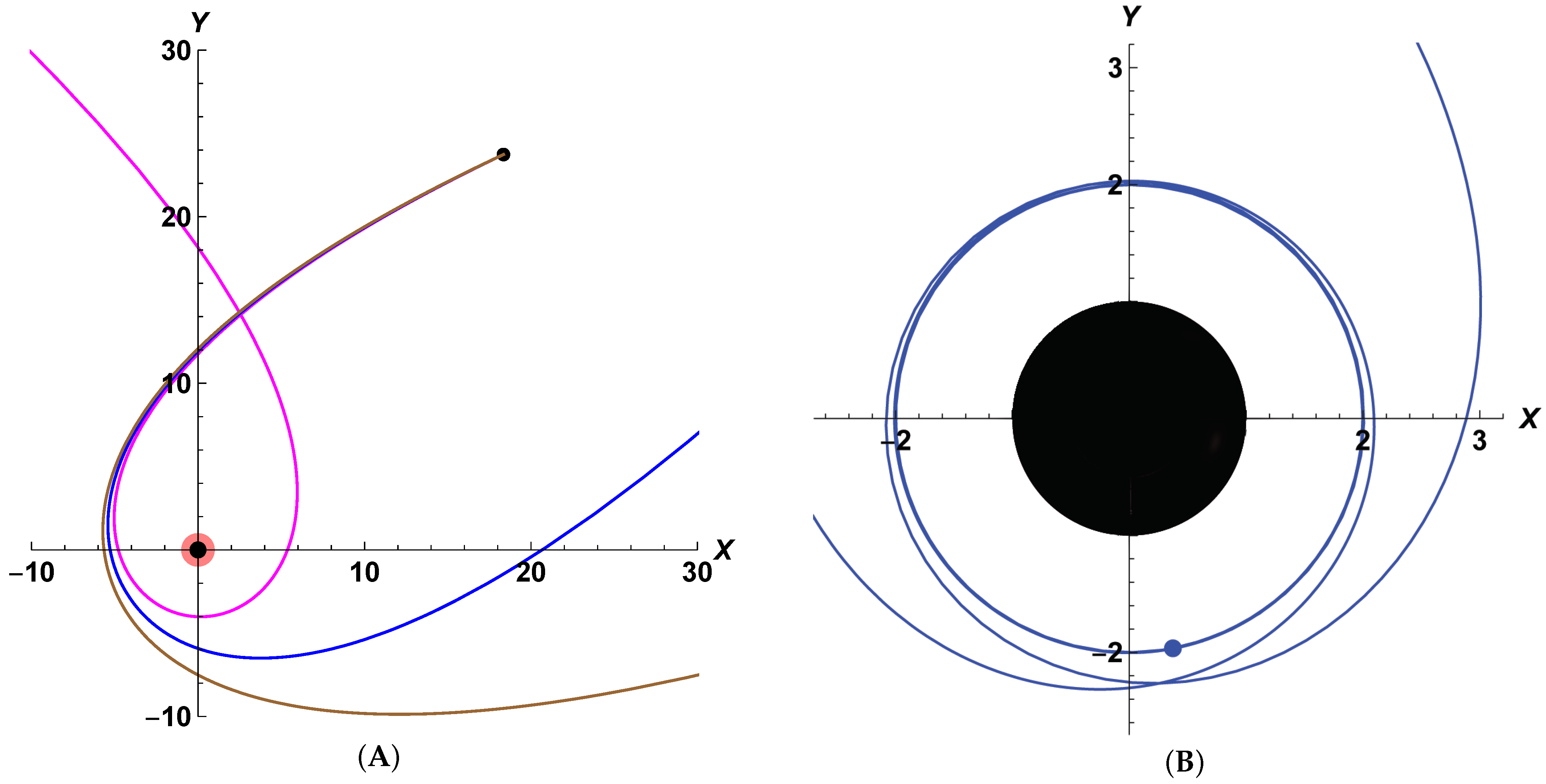
The shapes of the test-body’s trajectory within the zone of significant black hole influence (strong relativistic effects) may vary dramatically. Figure 1A illustrates the variety and plots trajectories of a test-body with (sufficient to escape in each case) for the scenarios when the black hole’s spin and the test-body’s momentum are co-aligned (, magenta line), counter-aligned (, brown line), and when the black hole does not spin at all (, blue line). As revealed, depending on the black hole’s spin, the trajectory may twist significantly (as shown by the magenta line, ), or quasi-reverse (as shown by the blue line, ), or simply curve (as shown by the brown line, ). When the black hole’s spinning is co-aligned with the body’s angular momentum, the movement of the body and the swirling of the time-space coincide. The essence of the effect may perhaps be grasped by visualizing a boat sailing with an ocean current or against the current—the boat’s trajectories relative to a distant observer would look quite different.
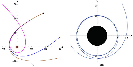
Figure 1.
Trajectory distortions for an object traveling with initial angular momentum j in the vicinity of a black hole (BH) with “rotation rapidity” : when BH spin and momentum j are co-aligned, BH spin is counter-clockwise; when BH spin and momentum j are counter-aligned, BH spin is clockwise. When , BH “radius” is (in the equatorial plane ) and ergosphere “radius” (pink) is 1. (Left Panel (A)) Impact of BH spin direction is shown for: (brown); (blue); (magenta). (Right Panel (B)) Dark-blue-trajectory (for ) illustrates temporary “capture onto quasi-circular orbit”: spiraling inward, passing through the periastron (Dark-Blue-Dot), and spiraling outward.
Particularly intriguing cases may occur when the initial angular momentum of the traveling body falls within a “narrow” range (not-too-fast but not-too-slow, defined by the system’s parameters; here ). For a non-spinning black hole (), the body may circle around the non-rotating black hole several times before departing towards infinity.
Figure 1B shows such trajectory’s details (recall that for a non-rotating black hole, the event-horizon coincides with the static limit). The Dark-Blue-Dot (in the lower-right quadrant of Figure 1B) corresponds to the minimal distance (periastron) from the “center” of the black hole that is reached by the body. As the body passes through the periastron (Dark-Blue-Dot), its radial velocity turns to zero. Prior to passing through the periastron, the sign of the body’s radial velocity component is negative (the body is approaching); after the passing, the sign is positive (the body is moving away). If the energy diagram were drawn, the process would look as if the representative point was moving along the straight line (of constant energy), reaching the energy barrier (corresponding to Dark-Blue-Dot in Figure 1B), reflecting from the barrier (passing trough the periastron), and moving in the opposite direction along the level of constant energy. (A similar discussion and underlying details can be found in [17].) This explains the gradual spiraling of the trajectory closer towards the periastron (Dark-Blue-Dot) and the subsequent unwinding. Eventually, the body departs the black hole’s vicinity and generally the zone of influence.
3.3. Strong Shift
By comparing observational data (periastron shifts) for star trajectories near black holes with theoretical curves for a range of spin-values , it may be possible to estimate the actual black hole spin. Since relativistic effects are the strongest at periastron when the orbit of a star (test-body) is not quasi-circular but elongated (quasi-parabolic), observations of elongated orbits can be more revealing than data on quasi-circular orbits. Consequently, in this section, we demonstrate how to calculate the shift of the periastron for a parabolic trajectory (energy ) and provide the results from our numerical simulations for a sample of spin-values .
When a star begins its travel from infinity (where its radial inverse-coordinate ) and approaches a black hole along the incoming (upper) branch of the trajectory, the star’s angular coordinate , for each u, is derived (as a function of the radial coordinate ) from Equation (23) and has the form
Here, is the value of u when solutions and merge (at the point where ). Parameter . Quantities and with are the solutions of equation
Solution determines the periastron in which derivative .
Realization Domain: Not every combination of is realizable. For example, as mentioned earlier, when the test-body’s initial angular momentum is below , the body becomes captured by the black hole (its trajectory ends at the static limit). So those test-bodies, which can eventually complete their trajectories, without being captured, are described by the combinations within a limited “realization” domain. Such domain has two bounds: and .
The (initial) bound, , is obvious and reflects the fact that the test-body starts at the infinity with some initial angular momentum . (Because Lagrangian is invariant with respect to rotation, the test-body’s angular momentum is conserved, so momentum remains constant as the test-body approaches the black hole along the incoming branch of the parabolic trajectory with energy .)
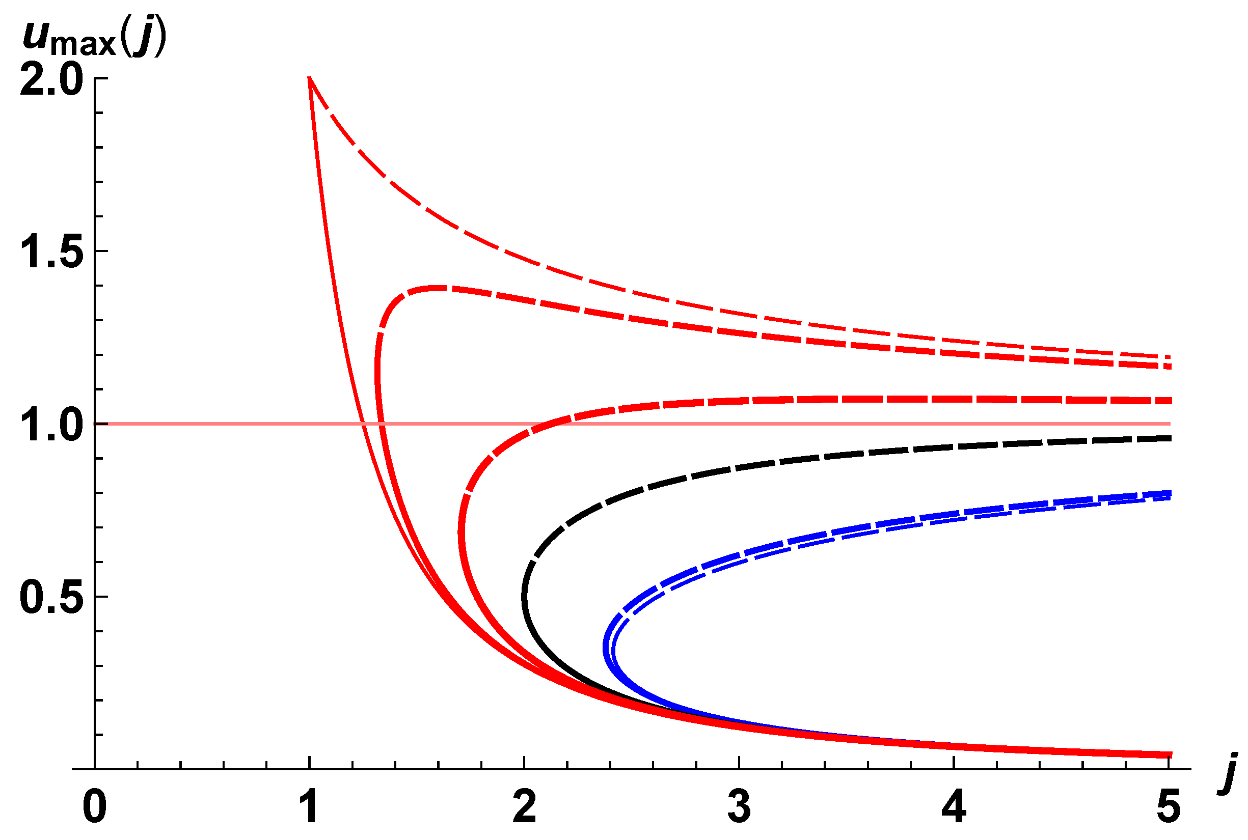
The second (periastron) bound, , is more complex. Figure 2 plots several u-curves composed of a solid part and a dashed part —merging at —but it is the curves’ lower branches (, solid lines) that serve as the second (periastron) bounds . (The curves are plotted for the black hole spin-values , from the left-most to the right-most: red , , ; black ; blue , ).
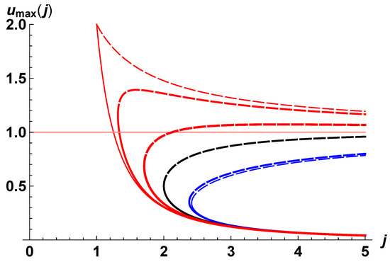
Figure 2.
Not every combination of is realizable. Trajectories are completed only when, for a given initial angular momentum , values u are within the “domain of physical motion”: between and . Colored u-curves, composed of branches (lower, solid) and (upper, dashed), correspond to scenarios with BH spin-values (from the left-most to the right-most): (red), (red), (red), (black), (blue), (blue). Horizontal line marks the static limit (where metric tensor component ). In this -space, the (corresponding to the test-body) state-point starts at the point and “moves” upward (along the vertical line ) until reaching —on the lower branch of the u-curve corresponding to the encountered black hole’s spin —which corresponds to the trajectory’s periastron in the physical space, then the body “reflects”, and returns downward (along the vertical line ) to point which is now the exiting value at the infinity.
For —which is the case when the test-body with initial momentum eventually escapes the black hole with spin —in the -space, the (corresponding to the test-body) state-point starts at the point and “moves” upward (along the vertical line ) until reaching the lower branch of one of the plotted u-curves (the one corresponding to the encountered black hole’s spin ). This point corresponds to the test-body’s trajectory’s periastron in the physical space. After the periastron, the test-body’s physical movement proceeds along the outbound branch of its physical trajectory, but in the -space, after “reflecting” at the periastron-representing state-point , the test-body-representing state-point follows the vertical line downward towards (now it is the exiting value at the infinity).
For the cases when the black hole captures the test-body and the body ends up falling onto the static limit (which happens when test-body’s initial angular momentum ), in the -space the test-body-representing state-point starts at the point and “moves” upward (along the vertical line ) until the horizontal line (the static limit, above which—within the ergozone—the metric-tensor component becomes negative).
Periastron Coordinates: The angular coordinate for periastron when (or for the body when it falls onto the static limit when ) is defined by the integral
where, for simplicity, the Heaviside function is used: when and when , with the half-maximum convention . We remind readers that in the region , quantity is purely imaginary, and in the region , is purely real and positive. The integral Equation (32) cannot be expressed in simple analytical functions. It can be either calculated numerically, or its asymptotics may be considered.
For large j, Equation (32) gives the following estimate
where only the leading terms are retained. The first term corresponds to classical Newtonian mechanics—the angular coordinate for the periastron is . The second term gives the shift of the periastron due to the relativistic effect in the Schwarzschild metric. This term is always positive. The third term takes into account the black hole’s spin and can have any sign. At , even for , this correction term is small when compared to the previous one, since for the Kerr metrics , always.
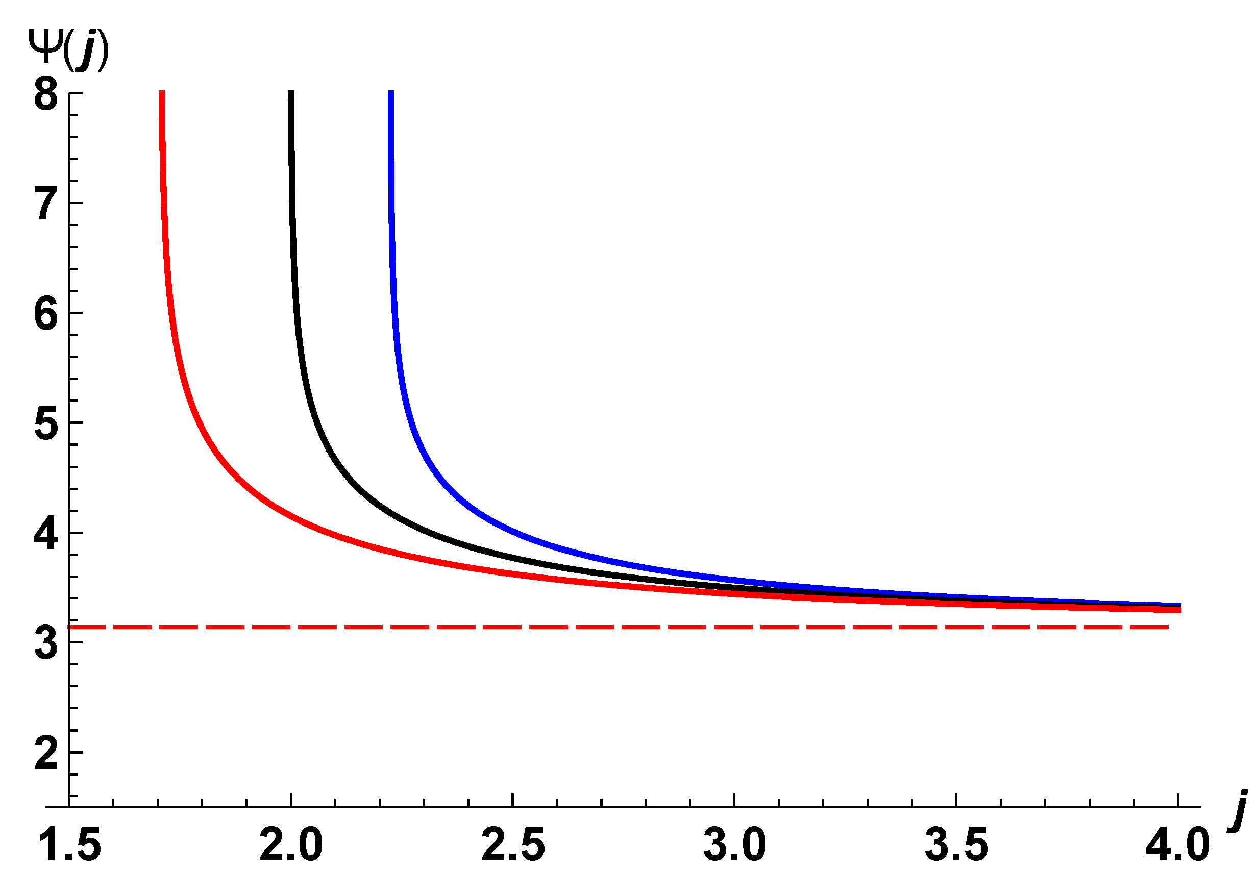
Figure 3 shows the angular coordinate for periastron as a function of test-body’s momentum j for three black hole spin-values: (blue), (black), and (red).

Figure 3.
Periastron coordinate as a function of the moment j for black hole spin-values : blue for , black for , and red for .
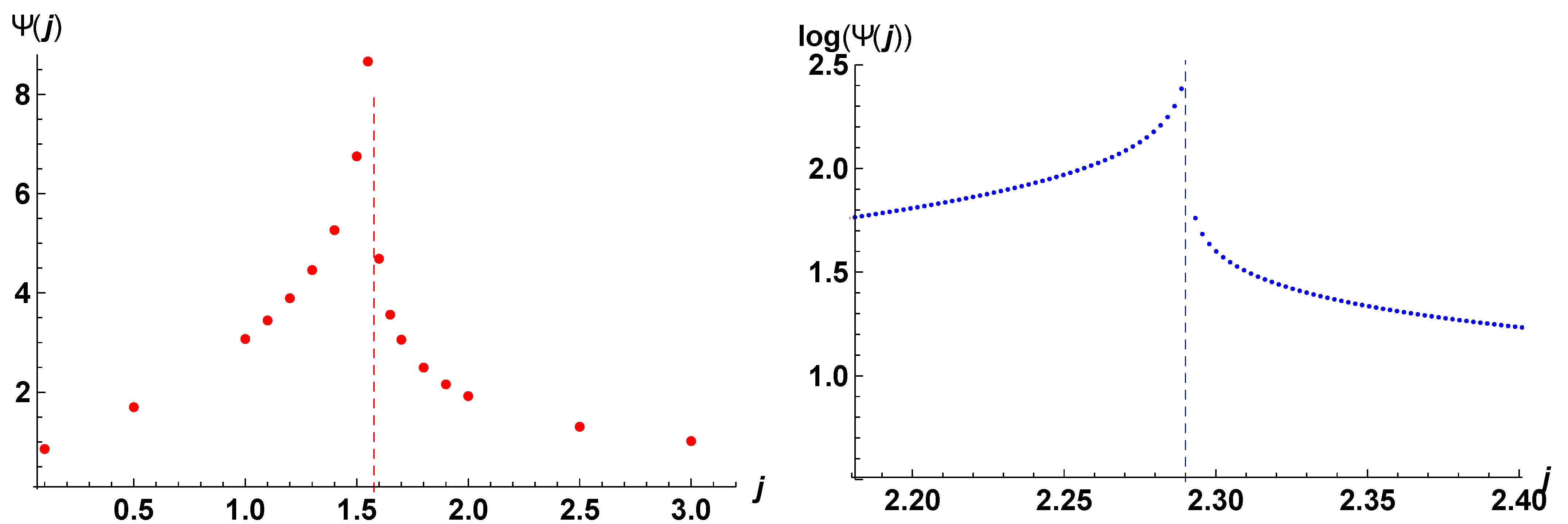
As Figure 3 reveals, for large values of initial angular momentum, , the relativistic effects are indeed relatively small, placing the periastron slightly above . However, the effect of the black hole’s spin becomes rather significant for . Notably, as shown in Figure 4, the effect is strongest for j near . The logarithmic scale in the right panel of Figure 4 reveals that -function is not some power-function but is more complex. The left panel shows the case when the black hole’s spin is counter-aligned () with the test-body’s angular momentum j. The right panel shows the case when the spin is co-aligned () with the momentum.
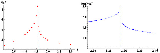
Figure 4.
(Left Panel) Numerical estimates of periastron coordinate for . (Right Panel) Numerical estimates of for .
In the vicinity of , integral diverges. By expressing momentum j as , where , and retaining only the leading terms, we find expression for in the vicinity of :
Here, and (which depend on ) are of order unity. For example, in the particular case of , the values of the parameters are: and . For , the value of the angular coordinate of the periastron turns out to be .
The total number, N, of rotations of the compact star around the black hole—seen as if “captured onto a quasi-circular orbit” by a remote observer—is then estimated as . (Here of rotations occur before the body reaches the periastron, and of rotations occur after passing through the periastron.)
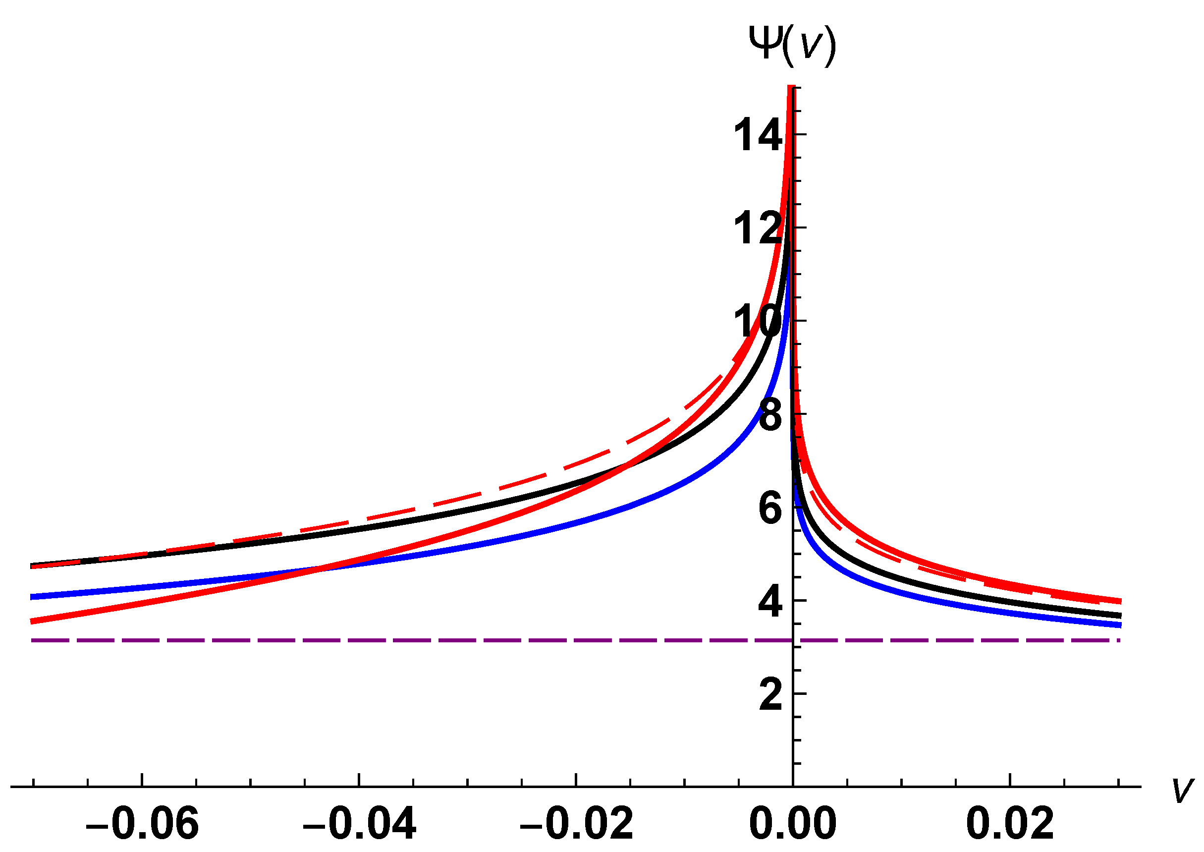
Finally, Figure 5 compares the locations and shapes of -curves when black hole spin is counter-aligned (, red), absent (, black), or co-aligned (, blue) with the test-body momentum j. Figure 6 reveals the nuances of the differences in the shapes of -curves when the test-body’s momentum-value happens to be in the vicinity of (i.e., near ). For comparison, the Newtonian periastron is plotted as the horizontal dashed line.
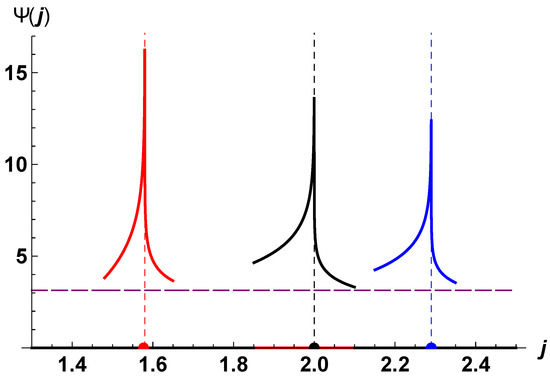
Figure 5.
Comparison of for black hole spin-values (red), (black), and (blue). Horizontal dashed line shows the Newtonian periastron .
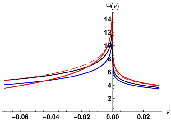
Figure 6.
Comparison of , where and , for black hole spin-values (red), (red dashed), (black), and (blue). Horizontal dashed line show the Newtonian periastron .
4. Conclusions
Context and Challenges: Measurement of the spin of certain black holes—such as, for example, the supermassive black hole closest to us, Sgr A*, at the center of our own Galaxy—may be challenging for a number of reasons. The geometry and temperature of their accretion disks may not produce X-ray reflection features or the thermal blackbody radiation suitable for analyses. When the black hole is single, no systematic gravitational waves are expected. Interpretations of the results from imaging with the Even Horizon Telescope—capable of detecting the asymmetry in brightness between the approaching and receding sides of the disk, which are strongly spin-dependent—may face model-dependent challenges due to time and space variability of the accretion disk and the foreground distribution of galactic matter that acts as a varying scattering screen. However, when it is possible to observe precession of highly-eccentric orbits of individual stars closely approaching the black hole, then the BH spin may be estimated. Over the past several decades, the existing—and continuously improving techniques—have been permitting such observations of individual bright stars traveling near Sgr A*. The relativistic shift of trajectory periastra—from which the BH spin value is deduced—would be even more pronounced for parabolic or hyperbolic stellar flybys.
Results: In this paper, we provide (1) analytical expressions for the periastron coordinate () for an elongated (parabolic/hyperbolic at the limit) trajectory; (2) numerical simulations and qualitative examinations of several illustrative scenarios; (3) discussion of the theoretical method permitting such comprehensive consideration; (4) illumination of the importance of symmetries of the Lagrangian and their contribution to construction of solutions; (5) illustration of the possibility of arising resonance regimes when test-bodies move in the vicinity of black holes. In particular, we find the relativistic shift of the periastron (relative to the Newtonian position, ), for varying rates of the black hole’s rotation : no-spin (, for comparison) and when the black hole’s spin is co-aligned () or counter-aligned () with the angular momentum (j) of the traveling star. It is shown that stars (modeled here as non-destructible compact test-bodies with zero initial kinetic energy at infinity) with the initial values of angular momentum () that are less than certain critical value () (which depends on , the spin of the black hole, as ) become captured by the black hole, while the stars with have their trajectories distorted by the black hole in various ways, but eventually return to infinity.
“Capture” onto Quasi-Circular Orbit: If the initial angular momentum happened to be less than the critical value for the spinning black hole, the black hole will capture the star—the star will spiral and inevitably fall onto the static limit. If , the star’s trajectory will curve around the black hole and the star will depart towards infinity. However, if the initial angular momentum happened to be close, but slightly more than the critical value for the spinning black hole, an interesting effect arises. After approaching the black hole, the star starts rotating around the black hole, gradually spiraling towards the periastron. It may take a great (finite) number of revolutions for the star to eventually reach and pass through the periastron point, at which moment that trajectory starts “unwinding” just as gradually. For the duration of this process, for an observer, the star would appear as if on a “circular” orbit close to the black hole, with radius . This radius can be observationally determined. Due to energy conservation, however, the star will eventually continue its journey along the outgoing branch of its trajectory, leaving the vicinity of the black hole, and exiting towards the infinity. Mathematically, the value for periastron coordinate becomes very large (Figure 4). At the limit , the angular coordinate of periastron tends to infinity according to logarithmic law (Equation (34)).
Practical Use: The obtained results may be of use in the following practical ways:
(1) Since these expressions are derived from the first principles for all orbits/trajectory types and for all black hole spins, the observations of periastron coordinates and measurements of angular momenta j can provide sufficiently accurate estimates for black hole spins :
Naturally, this formula is valid for . For j closer to , the analytical expression for involves cumbersome hyper-geometrical functions, and numerically estimated graphic representations (as illustrated in Figure 3, Figure 5 and Figure 6) offer easier visualization of its tendencies.
(2) Of particular interest may be the highly elongated orbits. The stars with such orbits spend the shortest amount of time in the vicinity of black holes and may be detected within much shorter observational timeframes than those required for quasi-circular orbits.
(3) The more elongated the orbit, the “sharper” the turn at the periastron, the greater the acceleration experienced by the traveling body. When acceleration is the highest, the (destroyed into charged “fragments”) body emits the maximum amount of electromagnetic radiation. Greater brightness makes it easier to detect astronomically and interpret theoretically. (synchrotron or bremsstrahlung radiation are the examples of this effect for charged particles.) Thus, elongated orbits offer the most promise for observations.
Novel Perspectives: Recently, the quest for measuring spins of supermassive black holes at the centers of galaxies has received an additional impetus. In the set of publications [20,21,22], we advanced and supported the hypothesis that an additional nucleogenetic process—fission-driven rather than nucleosynthesis-driven—contributes (and has historically contributed) to chemical enrichment of galaxies. This process depends (to a large extent) on the crushing and catapulting power of the central galactic black holes. More massive black holes with greater spins can catapult pieces of crushed neutron stars further, with greater speeds. Thus, the resulting distribution of the fission-driven nuclei-production relative to the nucleosynthesis-driven nuclei-production would differ between galaxies. See Ref. [20] for details. In our own galaxy, this fission-driven mechanism has impacted chemical compositions of stars, compositions and properties of exoplanets, structures of exoplanetary systems, and (not less importantly) the composition and structure of our own solar system (see Ref. [21]). To properly analyze the differences between chemical enrichments of galaxies, and to better understand the nucleogenetic signature of the fission-driven enrichment mechanism, accurate estimates of the masses and spins of central black holes are required.
Author Contributions
Conceptualization and writing, E.P.T. and V.I.P. All authors have read and agreed to the published version of the manuscript.
Funding
This research received no external funding.
Institutional Review Board Statement
Not applicable.
Informed Consent Statement
Not applicable.
Conflicts of Interest
The authors declare that there is no conflict of interest regarding the publication of this article.
References
- Reynolds, C.S. Observing Black Holes Spin. Nat. Astron. 2019, 3, 41–47. [Google Scholar] [CrossRef] [Green Version]
- Abuter, R.; Amorim, A.; Bauböck, M.; Berger, J.P.; Bonnet, H.; Brandner, W.; Cardoso, V.; Clénet, Y.; de Zeeuw, P.T.; Dexter, J.; et al. [GRAVITY Collaboration]. Detection of the Schwarzschild precession in the orbit of the star S2 near the Galactic centre massive black hole. Astron. Astrophys. 2020, 636, L5. [Google Scholar] [CrossRef] [Green Version]
- Parsa, M.; Eckart, A.; Shahzamanian, B.; Karas, V.; Zajaček, M.; Zensus, J.A.; Straubmeier, C. Investigating the Relativistic Motion of the Stars Near the Supermassive Black Hole in the Galactic Center. Astrophys. J. 2017, 845, 22. [Google Scholar] [CrossRef] [Green Version]
- Peißker, F.; Eckart, A.; Zajaček, M.; Ali, B.; Parsa, M. S62 and S4711: Indications of a Population of Faint Fast-moving Stars inside the S2 Orbit—S4711 on a 7.6 yr Orbit around Sgr A*. Astrophys. J. 2020, 899, 50. [Google Scholar] [CrossRef]
- Bambhaniya, P.; Solanki, D.N.; Dey, D.; Joshi, A.B.; Joshi, P.S.; Patel, V. Precession of timelike bound orbits in Kerr spacetime. Eur. Phys. J. C 2021, 81, 205. [Google Scholar] [CrossRef]
- Kerr, R.P. Gravitational Field of a Spinning Mass as an Example of Algebraically Special Metrics. Phys. Rev. Lett. 1963, 11, 237–238. [Google Scholar] [CrossRef]
- Misner, C.W.; Thorne, K.S.; Wheeler, J.A. Gravitation; W. H. Freeman and Company, Princeton University Press: Princeton, NJ, USA, 1973. [Google Scholar]
- Diener, P.; Frolov, V.P.; Khokhlov, A.M.; Novikov, I.D.; Pethick, C.J. Relativistic Tidal Interaction of Stars with a Rotating Black Hole. Astrophys. J. 1997, 479, 164–178. [Google Scholar] [CrossRef]
- Shapiro, S.L.; Teukolsky, S.A. Black Holes, White Dwarfs, and Neutron Stars; Wiley: New York, NY, USA, 2004. [Google Scholar] [CrossRef]
- Wiltshire, D.L.; Visser, M.; Scott, S.M. The Kerr Spacetime; Cambridge University Press: Cambridge, UK, 2009. [Google Scholar]
- Frolov, V.P.; Zelnikov, A. Introduction to Black Hole Physics; Oxford University Press: Oxford, UK, 2011. [Google Scholar]
- Thorne, K.S.; Blandford, R.D. Modern Classical Physics: Optics, Fluids, Plasmas, Elasticity, Relativity, and Statistical Physics; Princeton University Press: Princeton, NJ, USA, 2017. [Google Scholar]
- Landau, L.D.; Lifshitz, E.M. The Classical Theory of Fields; Elsevier: Amsterdam, The Netherlands, 2013. [Google Scholar]
- Neves, J.C.S. Deforming regular black holes. Int. J. Mod. Phys. A 2017, 32, 1750112. [Google Scholar] [CrossRef] [Green Version]
- Sharif, M.; Shahzadi, M. Neutral Particle Motion around a Schwarzschild Black Hole in Modified Gravity. J. Exp. Theor. Phys. 2018, 127, 491–502. [Google Scholar] [CrossRef]
- Tito, E.P.; Pavlov, V.I. Relativistic Motion of Stars near Rotating Black Holes. Galaxies 2018, 6, 61. [Google Scholar] [CrossRef] [Green Version]
- Landau, L.D.; Lifshitz, E.M. Mechanics; Elsevier: Amsterdam, The Netherlands, 1982. [Google Scholar]
- Ritus, V.I. Lagrangian equations of motion of particles and photons in a Schwarzschild field. Physics-Uspekhi 2015, 58, 1118. [Google Scholar] [CrossRef]
- Sharif, M.; Shahzadi, M. Particle dynamics near Kerr-MOG black hole. Eur. Phys. J. C 2017, 77, 363. [Google Scholar] [CrossRef]
- Tito, E.P.; Pavlov, V.I. “In-System” Fission-Events: An Insight into Puzzles of Exoplanets and Stars? Universe 2021, 7, 118. [Google Scholar] [CrossRef]
- Tito, E.P.; Pavlov, V.I. Hypothesis about Enrichment of Solar System. Physics 2020, 2, 213–276. [Google Scholar] [CrossRef]
- Tito, E.P.; Pavlov, V.I. Hot super-dense compact object with particular EoS. Astrophys. Space Sci. 2018, 363, 44. [Google Scholar] [CrossRef] [Green Version]

Publisher’s Note: MDPI stays neutral with regard to jurisdictional claims in published maps and institutional affiliations. |
© 2021 by the authors. Licensee MDPI, Basel, Switzerland. This article is an open access article distributed under the terms and conditions of the Creative Commons Attribution (CC BY) license (https://creativecommons.org/licenses/by/4.0/).