The Impact of Coronal Mass Ejections on the Seasonal Variation of the Ionospheric Critical Frequency f₀F2

Abstract

We investigated the relations between the monthly average values of the critical frequency (f₀F2) and the physical properties of the coronal mass ejections (CMEs), then we examined the seasonal variation of f₀F2 values as an impact of the several CMEs properties. Given that, f₀F2 were detected by PRJ18 (Puerto Rico) ionosonde station during the period 1996–2013. We found that the monthly average values of f₀F2 are varying coherently with the sunspot number (SSN). A similar trend was found for f₀F2 with the CMEs parameters such as the CME energy (linear correlation coefficient R = 0.73), width (R = 0.6) and the speed (R = 0.6). The arrived CMEs cause a plasma injection into the ionosphere, in turn, increasing the electron density, and consequently, f₀F2 values. This happens in the high latitudes followed by the middle and lower latitudes. By examining the seasonal variation of f₀F2, we found that the higher correlation between f₀F2 and CMEs parameters occurs in the summer, then the equinoxes (spring and autumn), followed by the winter. However, the faster CMEs affect the ionosphere more efficiently in the spring more than in the summer, then the winter and the autumn seasons.

1. Introduction

Several studies were interested in investigating the impact of solar activities upon the ionosphere [1,2,3,4]. Among those studies that are concerned with the response of the ionosphere critical frequency (f₀F2) to the coronal mass ejections (CMEs) has become of the utmost importance during the past few years [5,6,7]. Actually, the solar activity is the main source of disturbances and fluctuations in the Earth’s environment, in particular the magnetosphere and the ionosphere layers.

The variability of the ionosphere can be attributed to contributions from lower atmospheric internal waves, geomagnetic and solar activity variations from high atmosphere as well [8]. In fact, solar ionizing flux varies not only with a longer time scale, the solar cycle, but also with the shorter time scale, the quasi-27-day rotation of the Sun and even on a day to day basis. Additionally, solar flux-induced variations in the neutral temperature, winds and neutral composition manifest also to ionospheric plasma densities and heights [4].

Indeed, during solar minimum there is a little X-ray emission and a low number of CMEs, while at solar maximum the Sun’s atmosphere emits large amounts of X-rays in addition to large numbers of CMEs. This gives rise to a solar cycle variation in the intensity of ionization of the ionosphere. During solar storms, the ionospheric structure can be drastically modified by energy input from the Sun [9].

The ionosphere is separated into three layers D, E and F, in which the F layer is divided into two layers as well, F1 and F2. Moreover, the ionospheric electron density is highest around the F2 peak, and it has been the subject of many investigations.

The widely used f₀F2 is a well-defined parameter extracted from ionograms of ground-based ionosondes. Actually, f₀F2 has a strong solar activity dependence, but varies with the seasons. This may be attributed to thermospheric winds, neutral winds, dynamo electric fields as well as the distance between the Sun and Earth, which varies seasonally [5].

Nowadays, a general picture was drawn for the ionospheric dynamo, in which, the equatorial electrojet is produced due to Eastward electric field E [10] which interacts with Earth’s magnetic field B causing strong vertical upward E×B drift velocity and enhanced f₀F2 in low latitudes [11].

CMEs are thought to cause an increase of the electron density in large volumes of the Earth’s ionosphere [6]. In addition, CME events are usually the origin of intense geomagnetic storms and they occur predominantly during the solar maximum phase. That is why they are considered to be the origin of space weather effects [12]. Basically, CMEs are huge explosions of plasma and magnetic fields from the sun’s corona. They eject billions of tons of coronal material having frozen in magnetic fields which are greater than the background solar wind magnetic field (IMF). Additionally, they are travelling outward from the sun at speeds ranging from 250 (km/s) to as fast as near 3000 km/s.

Really, there were good efforts exerted by some researchers in the field such as authors of [6] who studied the direct influences of CMEs properties on f₀F2 at mid-latitude ionospheric stations during the period 1996–2013 and found that the energetic, massive and fast CMEs can affect f₀F2 more efficiently. Despite this, the authors of [4] found that both positive and negative deviations of f₀F2 have no dependency on season and location.

Moreover, authors of [7] studied the relation between the monthly-averaged values of CME parameters and the monthly maximum values of f₀F2 at high, middle, and low latitudes for solar cycles 23 and 24 and found that there is a moderately good correlation between the two time series graphs at high and middle latitudes, but the ionosphere correlation is not clear in lower latitudes, indicating that the impact of CMEs on f₀F2 is higher at high latitudes than at the low latitudes.

Besides, authors of [13] examined the effect of CMEs and solar winds on the seasonal variation of f₀F2 at the Korhogo station during the period 1992–2002, through investigating the geomagnetic activity index Aa, where Aa ≥ 40 nT during one, two or three days announcing the CMEs arrival based on studies of [14,15,16]. They reported that CMEs affect midday troughs on f₀F2 diurnal profiles and the night peaks in winter and spring. Nevertheless, in autumn, CMEs do not affect the nighttime peak on f₀F2 diurnal profiles. In addition, CMEs always causes stronger positive storms compared to the solar wind effects, assuming that these storms are mainly due to the combination of the phenomena of rapid penetration eastward electric field and equatorward neutral winds during daytime but at night time they are mainly related to neutral winds alone.

In the present work, we aim to examine the seasonal variation of f₀F2 as a response to the CMEs influences for a long time period (1996 to 2013) at middle latitudes. Besides, we would examine and explain which value of both the monthly average and the monthly maximum f₀F2 values which give better results concerning the response to the arriving CMEs. In the next section, we describe the data sources, while in Section 3 we introduce the methodology. Section 4 shows the results and discussions, and we give the conclusion in Section 5.

2. Data Sources

The ionospheric f₀F2 data were obtained from Space Physics Interactive Data Resource (SPIDR). The data span between 1996 and 2013, consisting of minutely values of f₀F2 with 5 min resolution.

Table 1. The details of the mid-latitude ionosonde station in the Northern hemisphere.

Code	Name	Latitude	Longitude
PRJ18	Puerto Rico	18.5°	−67.2°

summarizes the details of the selected station.

CME data were taken from the SOHO LASCO CME Catalog obtained from a URL (http://cdaw.gsfc.nasa.gov/CME_list/), we obtained 20635 CME events during the period 1996 to 2013.

3. Methodology

Before introducing a description of the methodology, it is preferred to give a brief note about the detection and the extraction of the data concerning with the ionospheric critical frequency and the coronal mass ejection. The basic idea of the performance of the ionosonde depends on that the ionization in the atmosphere is in the form of several horizontal layers, and consequently, the electron concentration varies with height. By broadcasting a range of frequencies, usually in the range of 0.1 to 30 MHz, and measuring the time it takes for each frequency to be reflected, it is possible to estimate the concentration and height of each layer of ionization.

The frequency at which the wave penetrates the layer without reflection is that the transmitted wave that just exceeds the peak plasma frequency or the critical frequency. The critical frequency is directly proportional to the square root of electron number density of the layer.

CMEs are massive plasma cloud associated with the magnetic field. We cannot observe the CME during its onset time of ejection because the solar disk is brighter than it. SOHO/LASCO satellite masks the solar disk, causing an artificial solar eclipse.

The CME can be shown as a cone beam that appear outside the occulting disk with a sky-plane angular width called “width” which is typically measured in the field of view (FOV) after the width becomes stable. The SOHO/LASCO catalog estimates the velocity, the mass and the energy corresponding to each CME which may eject in all directions around the sun.

Coronal mass ejections are considered as large eruptions of plasma and magnetic fields which are produced from various sources of high intensity plasma emission. These are often associated with the acceleration of energetic electrons. Energetic protons released by a CME can cause an increase in the number of free electrons in the ionosphere. The higher impact is in the high-latitude polar regions. The increase in free electrons enhances radio wave absorption. The higher impact is within the ionospheric D-region. It is leading to Polar Cap Absorption (PCA) events.

CMEs may reach Earth within one to five or even seven days according to their speeds [17,18,19,20,21,22] such that their prediction is so hard that no one can estimate their arriving time accurately and consequently their impact on the ionosphere. As a result, some scientists studied this impact by investigating some of certain events like [2,23,24]. On the other hand, others used the average values for the CMEs parameters and f₀F2 for a long time period to achieve a global and deep view upon the expected link between the CMEs and the ionospheric f₀F2 [6,7].

We have decided to use the same methodological invariants as that applied in [6] but with some modifications supporting our new goals in this study concerning the seasonal variation of f₀F2.

We estimated the monthly average values of the CMEs parameters and f₀F2 to overcome the problem of the inaccurate estimation of the CME’s travel time. In addition, we divided each year of data-taking into four seasons according to the meteorological temperate seasons as shown in

Table 2. The seasons according to meteorological temperate seasons.

The Seasons		The Period
Northern Hemisphere	Southern Hemisphere	Start	End
Winter	Summer	1 December	28 February
Spring	Autumn	1 March	31 May
Summer	Winter	1 June	31 August
Autumn	Spring	1 September	30 November

.

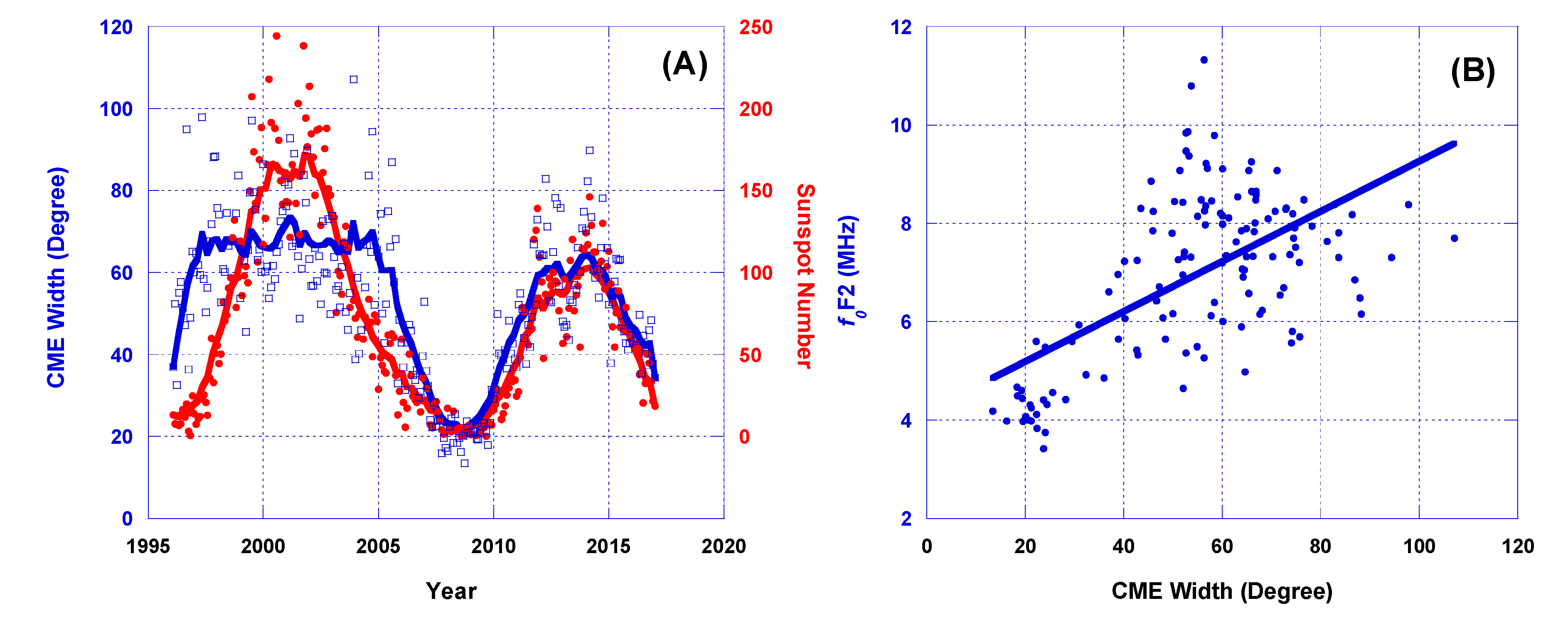
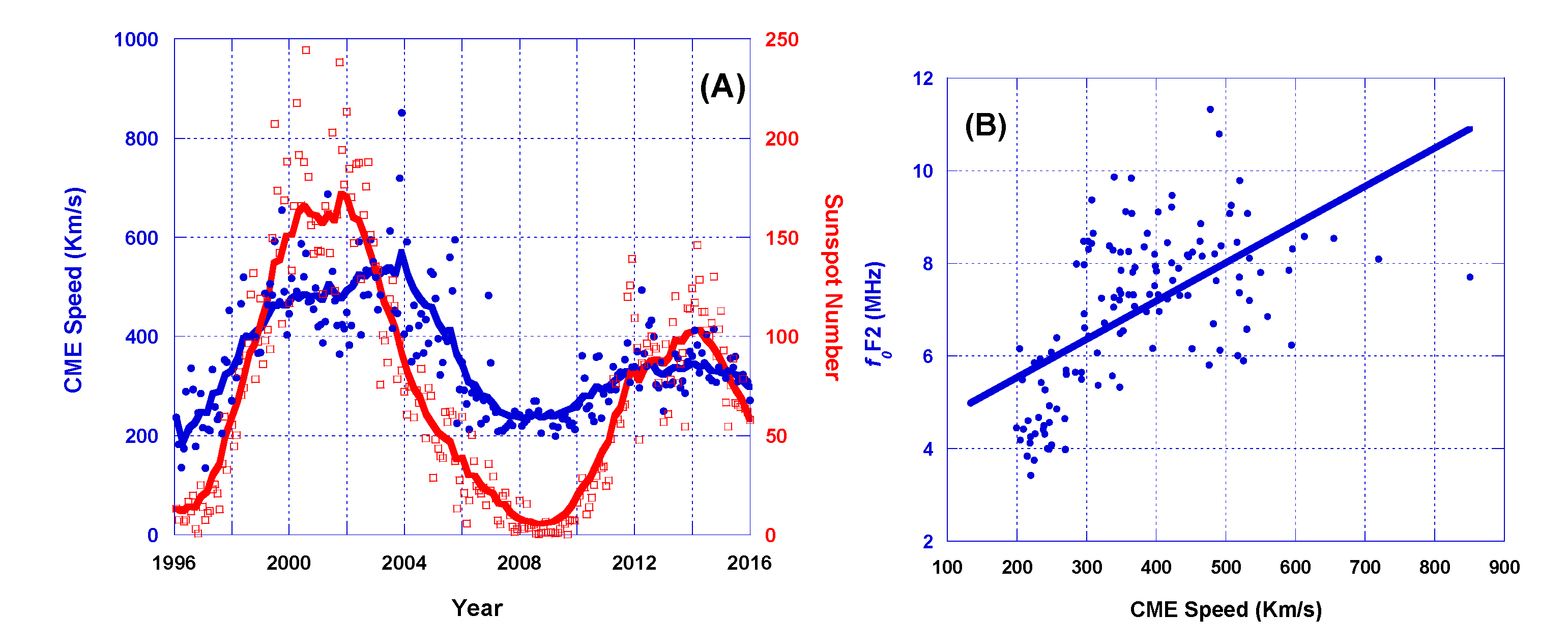
4. Results and Discussion

4.1. Monthly Variation

The monthly average value of f₀F2, hereafter F, changes drastically, exhibiting frequent oscillations, with time. In addition, we found that the monthly average value of f₀F2 profile has a high coherence with that of the sunspot number (SSN) as shown in Figure 1, we found that its profile has the maximum and the minimum monthly average values 11.3 MHz and 3.4 MHz at the dates May 2000 and July 2007 respectively.

Moreover, we examined the average and maximum monthly values of f₀F2 during our selected period. We found that the preferable matching with SSN profile is the monthly average values of f₀F2 as shown clearly in Figure 1 as well.

Using the monthly average f₀F2 provides more accurate results than the monthly maximum, different from the previous studies performed by [6,7] which focused on using the maximum value of the critical frequency, that is referring to the day-time variation in the ionosphere only. However, the average values more precisely reflect the total variation throughout the day, the day and the night, which implies, to a great extent, that the total incoming forces by the solar particles which may enhance at the night in the absence of the solar radiation. Therefore, we have decided to use the monthly average f₀F2 values in the present study in order to yield the improved outcomes.

CMEs represent an important portion of energetic particles and massive plasma coming from the Sun. Because of this, we plotted the monthly average values of the CMEs widths with F values as shown in Figure 2. This figure shows clearly that the CME angular width is varying with the solar activity as well as f₀F2. The widths become smaller during the quiet Sun phase, while they are greater during the active Sun phase. At the same time, F values become smaller during the quiet phase of the Sun and higher through the active phase of the Sun.

Actually, F values are linearly proportional to the monthly average values of the CME widths, providing the correlation coefficient R equals 0.6 (Pearson’s chi-squared test χ2 equals 244.01) according to the following equation:

F (MHz) = 4.1647 + 0.051 × W (degree)

(1)

where F is the monthly average value of f₀F2 (in MHz), and W is the monthly average value of the CME angular width (in degrees).

According to Figure 2, f₀F2 and CME width profiles match with the solar cycle 23 and the ascending period of the solar cycle 24. This trend emphasizes that the f₀F2 profiles rely, for a great extent, on the solar activity, which is in a good agreement with several works such as [3,5,25] and in particular the CMEs, as presented by [6,7,13]. One step further, Figure 1 and Figure 2 imply with no doubt that the less wide CMEs predominantly reach the Earth and can affect the ionosphere, such that the majority of CMEs, having angular widths less than 120 degrees, seem to have a similar f₀F2 time profiles. However, the wider CMEs have the ability to cause a plasma injection into the ionosphere than the thinner ones, in turn, increasing the electron density, or f₀F2. Obviously, this happens in the high latitudes followed by the middle and lower latitudes.

Although the time profile of the monthly average values of the CME parameters expresses a high coherence with SSN, including the CME energy, we found that the correlation of the monthly maximum value of the CME energy with the monthly average value of f₀F2 gives better results, as an exception, than using the monthly average CME energy.

Among the CME parameters, the CME energy seems to be the main factor that directly affects the ionosphere through ion production and consequently the critical frequency. Hence, the monthly maximum CME energy values give better results instead of the average ones, which indicates that the solar particles have a direct effect on the ionosphere.

Really, the maximum value of f₀F2, which is measured through the day only, expresses its response to both solar ionizing by radiation, in addition to other factors relating to the lower atmosphere. However, the average value of f₀F2, which is measured throughout the day and the night represents its response mainly to the solar plasma, in addition to other factors from the lower atmosphere.

As a consequence, and in order to investigate the CMEs energy influences upon f₀F2, we plotted the relation between the monthly maximum CME energy and the monthly average f₀F2 as shown Figure 3, which displays obviously a linearly direct correlation based on the following equation:

F (MHz) = 4.1127 + 4.1×10⁻⁴ × E (erg)

(2)

where E is the monthly average value of CME energy (erg). The correlation coefficient R equals 0.73 (Pearson’s chi-squared test χ2 equals 178.85). This high value indicates that the CME energy strongly affects the ionospheric critical frequency.

Along the same lines, the initial speed of CME increases directly with the solar activity. In general, the CMEs become faster through the active Sun phase and slower during the quiet Sun phase. This arises from investigating the relation between the CME speeds and the sunspot numbers, SSN as shown in Figure 4. Furthermore, the monthly average of CME initial speed has a linear correlation with the monthly average f₀F2, and the following formula represents its fitting:

F (MHz)= 3.88 + 8.26 ×10⁻³ × V (Km/s)

(3)

where V (Km/s) is the monthly average value of CME speed. The correlation coefficient R equals ∼0.6 (Pearson’s chi-squared test χ2 equals 246.12). This high correlation coefficient implies that the faster CMEs can affect the f0F2 more efficiently than slower ones.

Although the polynomial fitting gives a higher correlation coefficient than the linear fitting in our past figures. We preferred using linear correlation in order to make the investigations clearer and the results to be comparable in an obvious behavior. Specially, the second order polynomial fitting is very close to the performed linear fitting.

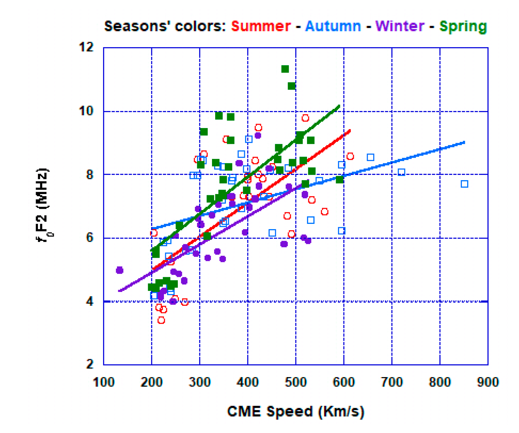
4.2. Seasonal Variation

The solar energy that leads to the ion production in the ionosphere is attributed not only to the solar radiation, but also to the solar particles [26]. This fact is generally valid during all seasons, but may be strong or slightly varying according to the season, in other words, the seasonal variation. These seasonal variations. These, in general, occur due to the tilt in the rotation axis of the Earth and the rotation of the Earth around the Sun. As a result, the Earth leans toward the Sun in the summer while it leans away from the Sun in winter, the equinox occurs in between as well. During the summer, the northern hemisphere, especially high latitudes, receives more solar radiation than the southern hemisphere due to the tilt angle and vice versa in the winter for the same northern hemisphere. This situation is similar in the case of solar plasma, including the solar wind and CMEs. In other words, during the summer season, the northern hemisphere, especially high and mid-latitudes, is subjected to plasma injection more than during the winter season.

Actually, the terrestrial northern hemisphere faces the heliospheric equator in the summer, which inclines by ~7.25° on the ecliptic, as a result, one can expect that the CMEs parameters can affect f₀F2 values in the mid-latitude region, tropical zone, in the summer season more efficiently than the spring and the autumn then the winter.

Figure 5 introduces a sketch which illustrates the impact of the Earth’s inclination with respect to the ecliptic plane on the area hit by the solar plasma. It shows clearly that the shorter path of the CME’s plasma is to the pole and it occurs during the summer season, while the middle path happens through the equinoxes, spring and autumn, and the longer path occurs during the winter season.

Figure 6 shows a high correlation between the monthly average CME energy and the monthly average f₀F2, which exhibits seasonal variation: (R = 0.76) in summer, (R = 0.64) in winter, (R = 0.59) in spring, then (R = 0.35) in autumn, in the northern hemisphere. However, we found that using the monthly maximum values of CME energy gives better results and the correlation coefficient values R increase as follows: (R = 0.82) in summer, (R = 0.80) in autumn, (R = 0.75) in spring, then (R = 0.67) in winter. Additionally, The CMEs width and initial speed display a similar seasonal variation trend as shown in Figure 7 and Figure 8, but with slight discrepancies: for the CMEs width, the correlation coefficients are (R = 0.69) in summer, (R = 0.68) in spring, (R = 0.62) in autumn, then (R = 0.60) in winter, in the northern hemisphere. At the same time, for the CME speed, the correlation coefficients are (R = 0.72) in spring, (R = 0.65) in winter, (R = 0.64) in summer, then (R = 0.46) in autumn, in the northern hemisphere.

Table 3. The correlation coefficient values (R) and Pearson’s chi-squared test χ2 of the linear relations between the monthly average f₀F2 and each of the monthly maximum CME energy and the monthly average values of the CME width and speed.

Seasons	Max CME Energy		Average CME Energy		CME Width		CME Speed
	R	χ2	R	χ2	R	χ2	R	χ2
Winter	0.67	33.244	0.64	36.431	0.61	38.765	0.65	35.593
Spring	0.75	52.89	0.59	79.476	0.68	64.845	0.72	58.644
Summer	0.82	31.656	0.76	41.242	0.69	51.213	0.64	57.484
Autumn	0.80	21.987	0.35	55.283	0.62	38.906	0.46	49.43

summarizes the values of the correlation coefficients R.

Actually, our selected ionosonde station is in the northern hemisphere of the Earth, localized approximately in the middle latitudes. Therefore, the correlation is the strongest in the summer season which may be attributed to that the number of electron density varies not only seasonal but also with respect to the latitudinal variations. However, the CME speed has a behavior that is different from the CME energy and width. The highest impact happens during equinoxes in the spring season, and this impact increases in the autumn season. This finding is also supported by the fact that the rate of electron density in equinox is faster than that in winter and summer season which leads to higher TEC at equinox months. Further, during this period, the Sun is directly above the equator, which leads to a higher value of TEC during the equinox at low latitude regions than at mid or high latitude [27].

5. Conclusions

The data of f₀F2 used in this work were collected from the ionosonde station PRJ18 (Puerto Rico) located approximately in the mid-latitude region. We estimated the monthly average values of f₀F2 during the period 1996–2013 and the corresponding monthly average values of the CME’s parameters.

By investigating the average and the maximum monthly values of f₀F2, we pointed out that the most preferable values, giving better results, are the monthly average ones. The average values reflect the total variation in the electron density throughout the day and the night that indicates the total incoming forces by solar particles.

We also found that the monthly average value of f₀F2 changes dramatically with time. It has a high coherence with the sunspot number (SSN). This behavior emphasizes that the f₀F2 profiles rely, for a great extent, on the solar activity.

Moreover, CME’s parameters are found to be varying with SSN in the same coherence behavior, like f₀F2. Further, by examining the correlations between each of the monthly average values of the CMEs’ physical properties and that of f₀F2, throughout the period of study, we found that relations are linear with the correlation coefficients equal approximately to 0.73, 0.6 and 0.6 for the CME energy, angular width and initial speed respectively.

The wide CMEs are more frequent during the active Sun, while they become less frequent during the quiet Sun. The CMEs’ speed and energy exhibit a similar behavior with the solar activity as well. As a result, the wider, energetic, and faster CMEs can increase the electron density in the ionosphere due to the plasma injection, giving rise to high values of f₀F2.

We also conclude that the highest impact of the CMEs on the seasonal variation is found to be in the summer, then equinoxes (spring and autumn) followed by winter. This is attributed to the direction of the Earth’s inclined rotational axis, with respect to the heliospheric equator.

During the summer solstice the terrestrial exposed area to the Sun is the greatest in the northern hemisphere, in addition, the north pole is the nearest one which has a shorter path for the plasma more than in the winter which has a longer path, giving rise to more plasma injection happening in the summer. This is valid for the CMEs energy and angular width. However, the CMEs speed shows a different behavior in which the faster CMEs raise the values of f₀F2 more efficiently in the spring, the winter and the summer, followed by the autumn season, respectively.

References

1. Liu, L.; Wan, W.; Ning, B.; Pirog, O.M.; Kurkin, V.I. Solar activity variations of the ionospheric peak electron density. J. Geophys. Res. Sp. Phys. 2006, 111. [Google Scholar] [CrossRef]
2. Iyer, K.N.; Jadav, R.M.; Jadeja, A.K.; Manoharan, P.K. Space Weather Effects of Coronal Mass Ejection. J. Astrophys. Astr. 2006, 27, 219–226. [Google Scholar] [CrossRef]
3. Kutiev, I.; Tsagouri, I.; Perrone, L.; Pancheva, D.; Mukhtarov, P.; Mikhailov, A.; Lastovicka, J.; Jakowski, N.; Buresova, D.; Blanch, E.; et al. Solar activity impact on the Earth’s upper atmosphere. J. Sp. Weather Sp. Clim. 2013, 3, A06. [Google Scholar] [CrossRef] [Green Version]
4. Buresova, D.; Lastovicka, J.; Hejda, P.; Bochnicek, J. Ionospheric disturbances under low solar activity conditions. Adv. Sp. Res. 2014, 54, 185–196. [Google Scholar] [CrossRef]
5. Ikubanni, S.O.; Adebesin, B.O.; Adebiyi, S.J.; Adeniyi, J.O. Relationship between F2 layer critical frequency and solar activity indices during several solar epochs. Indian J. Radio Sp. Phys. 2013, 42, 73–81. [Google Scholar]
6. Farid, H.M.; Mawad, R.; Yousef, M.; Yousef, S. The Impacts of CMEs on the Ionospheric Critical Frequency foF2. Elixir Sp. Sci. 2015, 80, 31067–31070. [Google Scholar]
7. Seyoum, A.; Gopalswamy, N.; Nigussie, M.; Mezgebe, N. The impact of CMEs on the critical frequency of F2-layer ionosphere (foF2). arXiv 2019, arXiv:2004.08278. [Google Scholar]
8. Yiǧit, E.; Immel, T.; Ridley, A.; Frey, H.U.; Moldwin, M. General Circulation Modeling of the Thermosphere-Ionosphere during a Geomagnetic Storm. 41st COSPAR Scientific Assembly, Abstracts from the the Meeting that was to be Held 30 July–7 August at the Istanbul Congress Center (ICC), Turkey, but was Cancelled. Abstract id. C1.1-1-16. Available online: http://cospar2016.tubitak.gov.tr/en/ (accessed on 27 October 2020).
9. Moldwin, M. An Introduction to Space Weather; Cambridge University Press: Cambridge, UK, 2008. [Google Scholar]
10. Seba, E.B.; Nigussie, M. Investigating the effect of geomagnetic storm and equatorial electrojet on equatorial ionospheric irregularity over East African sector. Adv. Sp. Res. 2016, 58, 1708–1719. [Google Scholar] [CrossRef]
11. Horvath, I.; Essex, E.A. The southern-hemisphere mid-latitude day-time and night-time trough at low-sunspot numbers. J. Atmos. Solar Terr. Phys. 2003, 65, 917–940. [Google Scholar] [CrossRef]
12. Gopalswamy, N. Coronal mass ejections and space weather. In Climate and Weather of the Sun-Earth System (CAWSES): Selected Papers from the 2007 Kyoto Symposium; Tsuda, T., Fujii, R., Shibata, K., Geller, M.A., Eds.; Terrapub: Tokyo, Japan, 2009; pp. 77–120. [Google Scholar]
13. Karim, G.; Jean, L.Z.; Kaboré, S.; Frédéric, O. Solar events and seasonal variation of foF2 at Korhogo station from 1992 to 2002. Int. J. Phys. Sci. 2020, 15, 22–27. [Google Scholar] [CrossRef]
14. Simon, P.A.; Legrand, J.P. Solar cycle and geomagnetic activity: A review for geophysicists. Part. I. The contributions to geomagnetic activity of shock waves and of the solar wind. J. Ann. Geophys. Atmos. Hydrospheres Space Sci. 1989, 7, 565–578. [Google Scholar]
15. Richardson, I.G.; Cane, H.V. Sources of Geomagnetic Activity during Nearly Three Solar Cycles (1972–2000). J. Geophys. Res. 2000, 107, 1187. [Google Scholar] [CrossRef]
16. Richardson, I.G.; Cliver, E.W.; Cane, H.V. Sources of Geomagnetic Activity over the Solar Cycle: Relative Importance of Coronal Mass Ejections, High-Speed Streams, and Slow Solar Wind. J. Geophys. Res. 2002, 105, 18203–18213. [Google Scholar] [CrossRef]
17. Gopalswamy, N.; Lara, A.; Yashiro, S.; Kaiser, M.L.; Howard, R.A. Predicting the 1-AU arrival times of coronal mass ejections. J. Geophys. Res. Sp. Phys. 2001, 106, 29207–29217. [Google Scholar] [CrossRef]
18. Owens, M.J.; Cargill, P. Predictions of the arrival time of Coronal Mass Ejections at 1AU, an analysis of the causes of errors. In Annales Geophysicae; Copernicus GmbH: Göttingen, Germany, 2004; Volume 22, pp. 661–671. [Google Scholar] [CrossRef] [Green Version]
19. Youssef, M.; Mawad, R.; Shaltout, M. Empirical Model of the Travel Time of Interplanetary Coronal Mass Ejection Shocks. NRIAG J. Astron. Geophys. 2011, 47–61. Available online: https://www.researchgate.net/publication/269518496_Empirical_Model_of_the_Travel_Time_of_Interplanetary_Coronal_Mass_Ejection_Shocks (accessed on 27 October 2020).
20. Mawad, R.; Youssef, M.; Yousef, S.; Abdel-Sattar, W. Quantized variability of Earth’s magnetopause distance, Quantized variability of Earth’s magnetopause distance. J. Mod. Trends Phys. Res. 2014, 14, 105–110. [Google Scholar] [CrossRef]
21. Mawad, R.; Farid, H.M.; Yousef, M.; Yousef, S. Empirical CME-SSC listing model. J. Mod. Trends Phys. Res. 2014, 14, 130–136. [Google Scholar] [CrossRef]
22. Mawad, R.; Radi, A.; Saber, R.; Mahrous, A.; Youssef, M.; Abdel-Sattar, W.; Hussein, M.; Yousef, S. Detection of interplanetary coronal mass ejections’ signature using artificial neural networks. J. Mod. Trends Phys. Res. 2016, 16, 1–10. [Google Scholar] [CrossRef]
23. Haider, S.A.; Abdu, M.A.; Batista, I.S.; Sobra, J.H.; Kallio, E.; Maguire, W.C.; Verigin, M.I. On the responses to solar X-ray flare and coronal mass ejection in the ionospheres of Mars and Earth. Geophys. Res. Lett. 2009, 36. [Google Scholar] [CrossRef]
24. Adebesin, B.O.; Ikupanni, S.O.; Ojediran, J.O.; Kayode, J.S. An investigation into the geomagnetic and ionospheric response during a magnetic activity at high and mid-latitude. Adv. Appl. Sci. Res. 2012, 3, 146–155. [Google Scholar]
25. Chaitanya, P.P.; Patra, A.K.; Balan, N.; Rao, S.V.B. Ionospheric variations over Indian low latitudes close to the equator and comparison with IRI-2012. Ann. Geophys. 2015, 33, 997–1006. [Google Scholar] [CrossRef] [Green Version]
26. Schunk, R.; Nagy, A. Ionospheres: Physics, Plasma Physics, and Chemistry, 2nd ed.; Cambridge Atmospheric and Space Science Series; Cambridge University Press: Cambridge, UK, 2009. [Google Scholar]
27. Parwani, M.; Atulkar, R.; Mukherjee, S.; Purohit, P.K. Latitudinal variation of ionospheric TEC at Northern Hemispheric region. Russ. J. Earth Sci. 2019, 19. [Google Scholar] [CrossRef]
Figure 1. The time series of the monthly average (A) and the monthly maximum (B) values of ionospheric critical frequency f0F2 (in MHz). The two plots are compared with the monthly average sunspot number, SSN showing a good agreement. The blue color of the left axis values, smooth curve and square points refer to f0F2 values, while the red color of the right axis values, smooth curve and round points denote to the sunspot numbers.
Universe 06 00200 g001
Figure 2. The time series of the monthly average values of the coronal mass ejections (CMEs) angular widths (in degrees) and that of the sunspot number (SSN) (A), and the relationship between monthly average value of f0F2 values and the monthly average CMEs widths (B). The blue color of the left axis values, smooth curve and square points of plot (A) refer to the CME’s width, while the red color of the right axis values, smooth curve, and round points denote to the sunspot numbers.
Universe 06 00200 g002
Figure 3. The time series of the monthly average values CME energy (in erg) and that of sunspot numbers (SSN) during the period 1996–2013 (A), and the relationship between F values and the monthly maximum CME energy (B). The blue color of the left axis values, smooth curve and round points of plot (A) refer to the f0F2, while the red color of the right axis values, smooth curve and square points denote to the sunspot numbers.
Universe 06 00200 g003
Figure 4. The time series of the monthly average values CME initial speed (Km/s) and that of the sunspot numbers (SSN) during the period 1996–2013 (A), and the relationship between F values and the monthly average CMEs initial speeds (B). The blue color of the left axis values, smooth curve and round points of plot (A) refer to f0F2 values, while the red color of the right axis values, smooth curve, and square points denote to the sunspot numbers.
Universe 06 00200 g004
Figure 5. A sketch shows the path of the CME’s plasma, through the magnetosphere, directed into the left panel (A): during the equinoxes; the middle panel (B): during summer for the southern hemisphere; the right panel (C): during summer for the northern hemisphere. The shortest path to the pole is during the summer season, while the longest one is during the winter season.
Universe 06 00200 g005
Figure 6. The seasonal variation of the monthly average f0F2 with the monthly average CME energy (left panel) and the monthly maximum CME energy (right panel). The season points and its fitting line are colorized as in the figure’s caption of each season word’s color.
Universe 06 00200 g006
Figure 7. The seasonal variation of the monthly average f0F2 as a response to the monthly average CME width variation. The season points and its fitting line are colorized as in the figure’s caption of each season word’s color.
Universe 06 00200 g007
Figure 8. The seasonal variation of the monthly average f0F2 as a response to the monthly average CME initial speed variation. The season points and its fitting line are colorized as in the figure’s caption of each season word’s color.
Universe 06 00200 g008