1. Introduction
Binary black hole (BBH) coalescences constitute one of the most important types of gravitational wave sources for the network of gravitational-wave detectors, such as the Advanced LIGO [
1], Virgo [
2,
3], GEO [
4], and KAGRA [
5], with the first observational detection of gravitational waves coming from precisely such a binary [
6]. Hence, it is important to know what dynamics of the astronomical system underlies the inspiral, merger and ringdown stages of a BBH waveform, and can therefore be studied using that waveform. For example, the merger phase (defined here as between the formation of the common apparent horizon, i.e., merger, and the beginning of the quasinormal mode ringdown) dynamics are interesting because they reflect strong gravity behaviors and correspond to a large gravitational wave amplitude.
The particular aspect of the merger phase dynamics we examine is the decline (not necessarily disappearance) of the current quadrupole moment relative to the mass quadrupole moment in the near zone. For our study, we will rely on
-symmetric simulations such as the superkick (equal-mass BBH with anti-aligned spins in the orbital plane) BBH coalescence previously examined in Reference [
7] for demonstration, which we will refer to as the SK simulation. By
-symmetry, we mean that the system is invariant under a
-rotation around an axis orthogonal to the initial orbital plane [
8]. This symmetry brings about significant simplifications that are useful for us. We will also utilize other
-symmetric simulations (not necessarily superkick configurations) whose initial parameters are similar to those of SK, aside from the initial spin orientations. The details of the initial parameters for these simulations are given in
Table 1 (note that these parameters are obtained at the very beginning of the simulation, on the initial data [
9]; once the simulation gets going, there will be a pulse of junk radiation emitted, as the system settles down from a caricature of the actual binary to a more accurate depiction, which subsequently leaves the computational domain; the parameters will change slightly after the junk radiation passes, and the binary will tend to pick up a slight eccentricity. Such changes will not affect the qualitative studies that are carried out in this paper, but please refer to [
10] for a more quantitative assessment of the impact of junk radiation; the simulations are carried out with resolutions comparable to the high resolution runs of the catalogue described in [
11]).
In this paper, weak field and/or perturbative expressions are utilized to help build intuition and aid in the formulation of qualitative arguments. However, we will use the tools of tendex and vortex, which are non-perturbative and valid in strong fields, to examine the numerical simulations. We begin by examining the analytical predictions for the tendex and vortex fields generated by the mass and current quadrupoles in
Section 2. We then use the knowledge gained to study these quantities in the SK simulation, and show that the current quadrupole declines in relative importance against the mass quadrupole during the merger phase. In
Section 3, we propose the mechanism through which the current quadrupole makes its exit, namely that the remnants of the individual spins become (nearly) aligned or anti-aligned with the total angular momentum. In
Section 4, we directly visualize the movements of these remnant spins using the horizon vorticity, which appear to be in agreement with our proposal. Finally in
Section 5, we speculate on the implication of our investigation in terms of helping the electric and magnetic parity quasinormal modes (QNM) achieve equality in their frequencies.
Note that the spin-total angular momentum alignment or anti-alignment considered here is not the same as the spin-flip examined in, for example, References [
12,
13], which considers the difference between the spin of the remnant black hole and the pre-merger individual spins (i.e., a comparison between different entities), and is simply a result of the former acquiring much of the pre-merger orbital angular momentum [
12]. Our discussion is, however, a comparison between the individual (remnant) spins with their earlier selves.
In the formulas below, the spacetime indices are written in the front part of the Latin alphabet, while the spatial indices use the middle part of that alphabet. We will use bold-face font for vectors and tensors, and adopt geometrized units with
. All the simulations and visualizations are performed with the Spectral Einstein Code (
SpEC) [
14] infrastructure.
2. Vorticity from the Mass and Current Quadrupoles
Given a timelike vector field
normal to a foliation of the spacetime by spatial hypersurfaces, the tendex
and vortex
fields are spatial tensors defined by:
where
is the Weyl curvature tensor,
is the projection operator into the spatial hypersurfaces with
being the spacetime metric, and the Hodge dual operates on the first two indices. Because the Weyl curvature tensor can be decomposed into and be reconstructed from the tendex and vortex fields, we can see these fields as representations of the spacetime geometry. The eigenvalues of
and
are called tendicities and vorticities. Because the tendex and vortex tensors are
matrices at each field location, there are three branches of tendicities and vorticities. From the discussions in Section VI of Reference [
15], we know that in the wave zone, one of the branches is associated with the Coulomb background piece of the Weyl curvature tensor, in the sense that the tendicity and vorticity are the real and imaginary parts of the Newman–Penrose (NP) scalar
(see Reference [
16] for more details on interpreting
—
in that paper —as the Coulomb background, and
—
in that paper—as the outgoing transverse radiation). We will refer to this branch as the Coulomb branch, even in the near zone. The other two branches weave into the gravitational wavefront in the sense of Figures 7 and 8 of Reference [
15], as well as Reference [
17]. Another definition we will need is the horizon vorticity. Given the spatial normal
to an apparent or event horizon, the horizon vorticity
is defined by
.
For the rest of the section, we will mostly specialize to the Coulomb branch vorticity field generated by the mass and current quadrupoles, although as the discussions are centered on symmetries, they would work with the other two branches as well. The mass quadrupole contains only orbital motion contribution; and is given by (for point particles, and for the leading terms in the usual post-Newtonian approximation; for higher order corrections, please consult, e.g., Reference [
18]):
where
labels the black holes and STF stands for taking the symmetric, trace-free part. The current quadrupole moment is given by:
with
being the total angular momentum that has two components: The orbital angular momentum and the spins:
For the
-symmetric simulations we consider, the
are the same for the two black holes, but the
are opposite, so the orbital contribution from the two black holes cancel out in Equation (
3). The spin contribution, on the other hand, have opposite
for the two black holes (
is the projection operator into the orbital plane, which for the post-merger context will refer to the equatorial plane of the remnant black hole), and therefore does not need to vanish. Furthermore, the total orbital angular momentum
and the total spin
are both collinear with
.
Note that Equations (
2) and (
3) are in the STF notation of Reference [
19,
20,
21], which has been summed over
m. For our simulations,
-symmetry suppresses the
modes, and even though there can be some small
mode contribution in the waveforms, we are most interested in the
modes. To approximate the
and
generating such modes in our simulations, we can use the quasi-Newtonian formula:
on a Cartesian coordinate system
with
spanning the orbital plane. The quantity
M is the total mass,
R is the separation between the black holes, and
is the Newtonian orbital angular frequency. Note that we have replaced the time
t in a purely Newtonian expression by the retarded time
. For the current quadrupole, there are a few interesting configurations. First of all, when the spins are constant, anti-parallel to each other and in the orbital plane, we have:
where
S is the shared magnitude of the individual spins. Note that as the spins don’t precess, there is only one
factor in Equation (
6) coming from the
term in Equation (
3), so the current quadrupole will evolve at the orbital frequency, instead of twice the orbital frequency like the mass quadrupole. If however, the spins precess also at frequency
, we would then have the current quadrupole evolving at a frequency of
. For example, in the simple case where the spins are anti-parallel, locked to orthogonal directions to the line linking the black holes, and confined to the orbital plane, we have:
Another useful result is for the case when spin
is locked to the
direction, where:
Finally, we note that if the two spins are aligned with each other, such as in the AA simulation (spins anti-aligned with the orbital angular momentum), then we suffer from the same effect that diminishes orbital contribution to
: The
are the same for the two black holes, while their
are opposite, so the overall current quadrupole vanishes. For the SK, SK- and SK⊥ simulations (spins initially in the orbital plane, see
Table 1), the current quadrupole moment is non-vanishing during inspiral, and can be approximated by Equation (
6) during the early part of inspiral. Towards later stages of inspiral, the spin precession frequency increases and
is somewhere between Equations (
6)–(
8). We now develop some tools for tracking how
evolves in, e.g., the SK simulation, during the merger phase.
The tendex and vortex fields corresponding to the current quadrupole
, in weak gravity, with a source region smaller than the gravitational wavelength, are given in Reference [
15] as:
where repeated indices are summed over, parentheses denote symmetrization, commas signify partial derivatives, and the overdot denotes time derivatives. Roughly, each time derivative introduces an
factor, while each spatial derivative can introduce either an
factor when operating on explicit
r’s in Equations (
9) and (
10), or an
factor through the retarded time. In the near zone, where
(ƛ is the reduced wavelength), the spatial derivatives that generate
factors are favorable, so terms with more spatial derivatives are more dominant, and the strength of the tendex and vortex fields are determined by the first terms in Equations (
9) and (
10). The ratio of the strength between them is proportional to
. When
(in the wave zone), it is preferable for spatial derivatives to introduce an
factor instead, and all the terms in the sums contribute equally. The result in the case of Equation (
9) is the same as a transverse-traceless projection operator acting on the four time derivative term multiplied by
. In this case, the
and
fields are of the same strength, as one would expect from them being sustained by mutual induction in a gravitational wave [
15].
The
and
fields generated by the mass quadrupole
have the same form as those due to the current quadrupole, up to prefactors, but with
and
swapped:
The symmetry between Equations (
9), (
10) and Equations (
11), (
12) allows for the definition of a complex quadrupole moment:
and then the tendex and vortex fields are given by the unified expression:
We now turn to examine the symmetry properties of the
field generated by Equations (
9) and (
11). Following Reference [
22], we define a positive/negative (abbreviated to +ve/−ve below) parity tensor field to be one that does not/does change sign under a reflection against the origin. Note that the parity operation we consider applies to the field location coordinates (e.g.,
r in Equation (
9), and not the source (black hole) locations or motions e.g.,
or
in Equation (
4), which can be seen formally as existing in a separate internal vector space. This is akin to applying the parity transformation to only the
x coordinate of a Green function
while leaving
unaffected. It is straightforward to see that both
and
have +ve parity, as do
in Equation (
9) and
in Equation (
12) that have even numbers of derivatives, while
in Equation (
10) and
in Equation (
11) take on −ve parity.
We show in
Figure 1 that the Coulomb branch vorticity contours for
as given by Equations (
9) and (
11). In addition to parity, our
fields are
-symmetric by construction. So by combining a
-rotation with a parity transformation, we arrive at reflection anti-symmetry/symmetry about the orbital plane, for the mass/current quadrupole generated vorticity. Furthermore, for the
modes we are considering, there is a
-rotation antisymmetry for both
and
generated vorticity, as evident from
Figure 1. We will call the combination of a parity transformation with a
-rotation the “skew-reflection”, and then the mass/current quadrupole generated vorticity is skew-reflection symmetric/anti-symmetric. Now consider an axisymmetric dipolar vorticity which also has a −ve parity, such as that generated by the orbital angular momentum or the spin of the post-merger final remnant black hole. It would be reflection anti-symmetric, as well as skew-reflection anti-symmetric. Therefore, a combination of the mass quadrupolar and the dipolar vorticities would have a definitive reflection anti-symmetry, but has no definitive skew-reflection symmetry property. Subsequently, the contours of opposite vorticities will be aligned with each other (in terms of rotation about the
axis) across the orbital plane. On the other hand, when we combine the current quadrupolar vorticity with the dipolar vorticity, we will have definite skew-reflection anti-symmetry, but no definitive reflection symmetry property. Therefore, the contours of opposite vorticities will be misaligned by
instead.
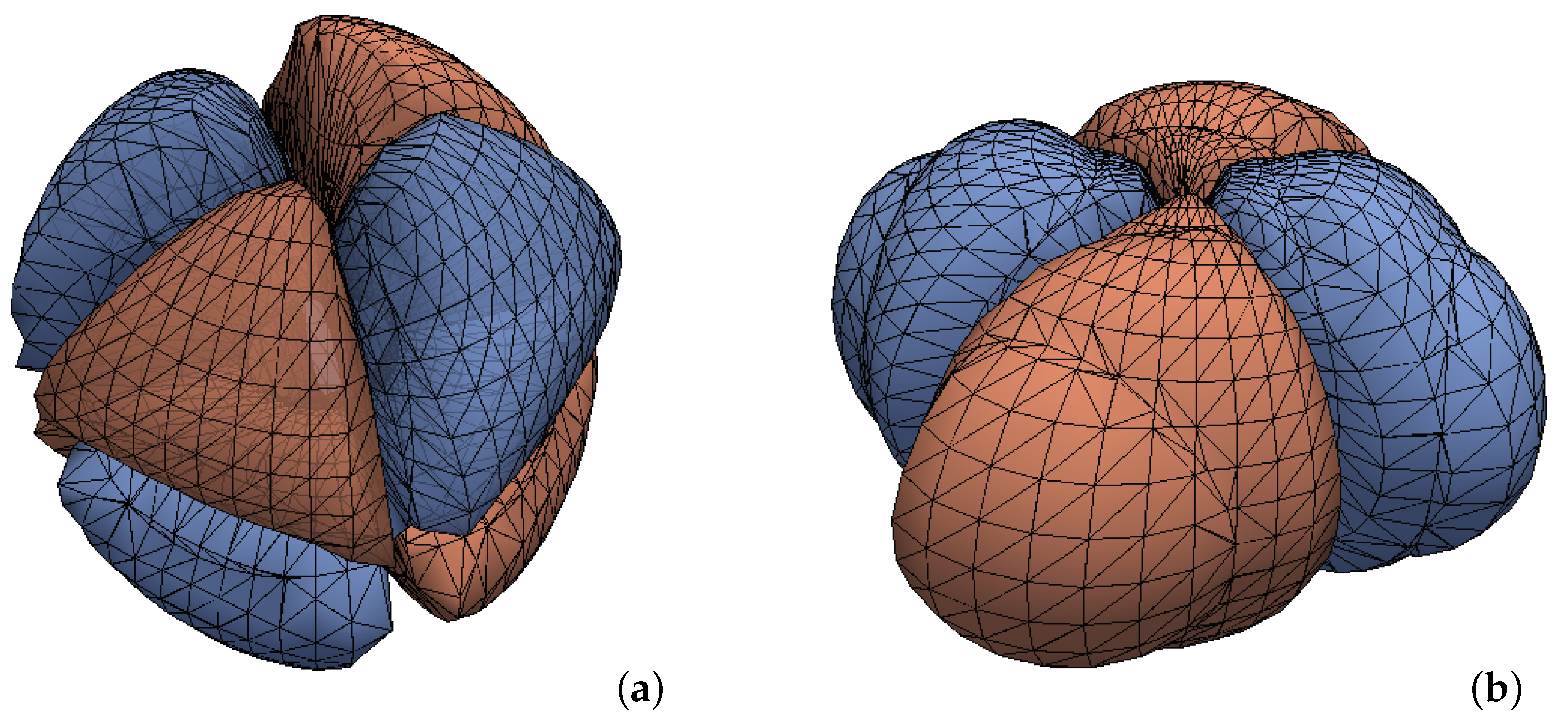
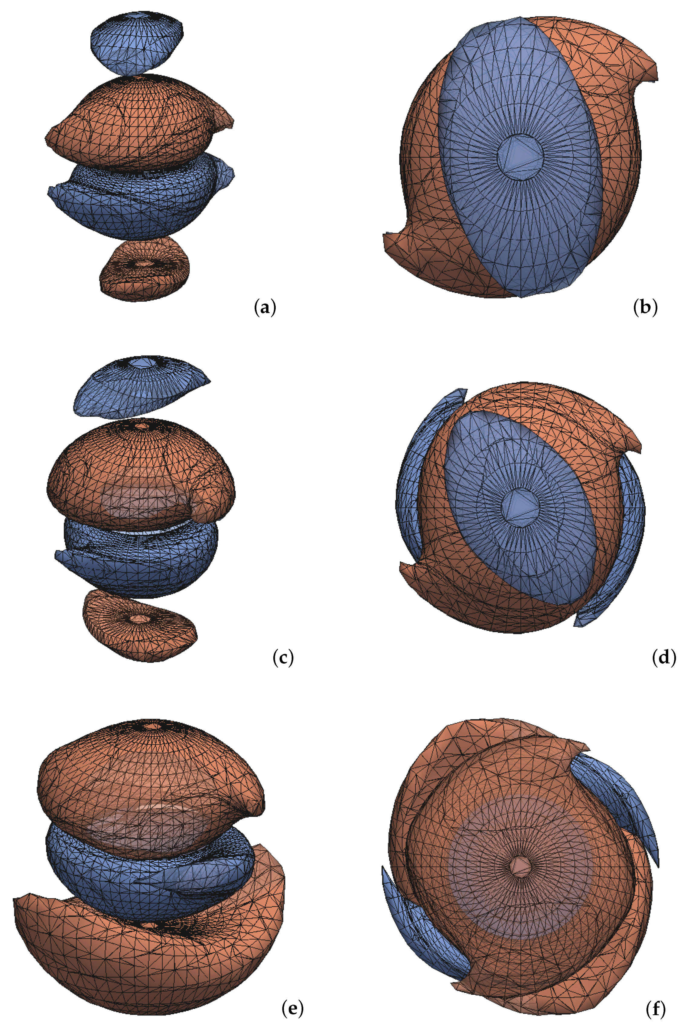
This conclusion is demonstrated graphically in the top two rows of
Figure 2, where contours of opposite vorticity are represented in red and blue. When constructing this figure, the dipole contribution is approximated as the vorticity field of a Kerr black hole [
23] in the Kerr–Schild coordinates (with spin
, similar to the final merged hole).When we combine the contributions from both quadrupoles (with parameters
,
,
and
) as well as the dipole, the red and blue spiraling arms subtend a misalignment angle between 0 and
(possessing neither definitive reflection symmetry nor definitive skew-reflection symmetry), as shown in the third row of
Figure 2. Note that although we have been utilizing weak gravity expressions in this section to construct examples, the qualitative symmetry considerations should remain valid in strong gravity, where this misalignment angle can serve as a convenient measure of the relative strength between the two types of quadrupoles. Aside from a non-vanishing misalignment angle, another indicator for the existence of a current quadrupole contribution is that the contours can slice through the orbital plane (see
Figure 1b and
Figure 2e), which is allowed by the skew-reflection anti-symmetry. On the other hand, reflection antisymmetry prevents the contours with non-vanishing vorticity from intersecting the orbital plane (see
Figure 1a and
Figure 2a). Finally, note that when both types of quadrupoles are present, the red and blue contours do not need to share the same size and/or shape (see
Figure 1e,f), with the difference between them dependent on the relative strength of these quadrupoles, as well as their relative phase.
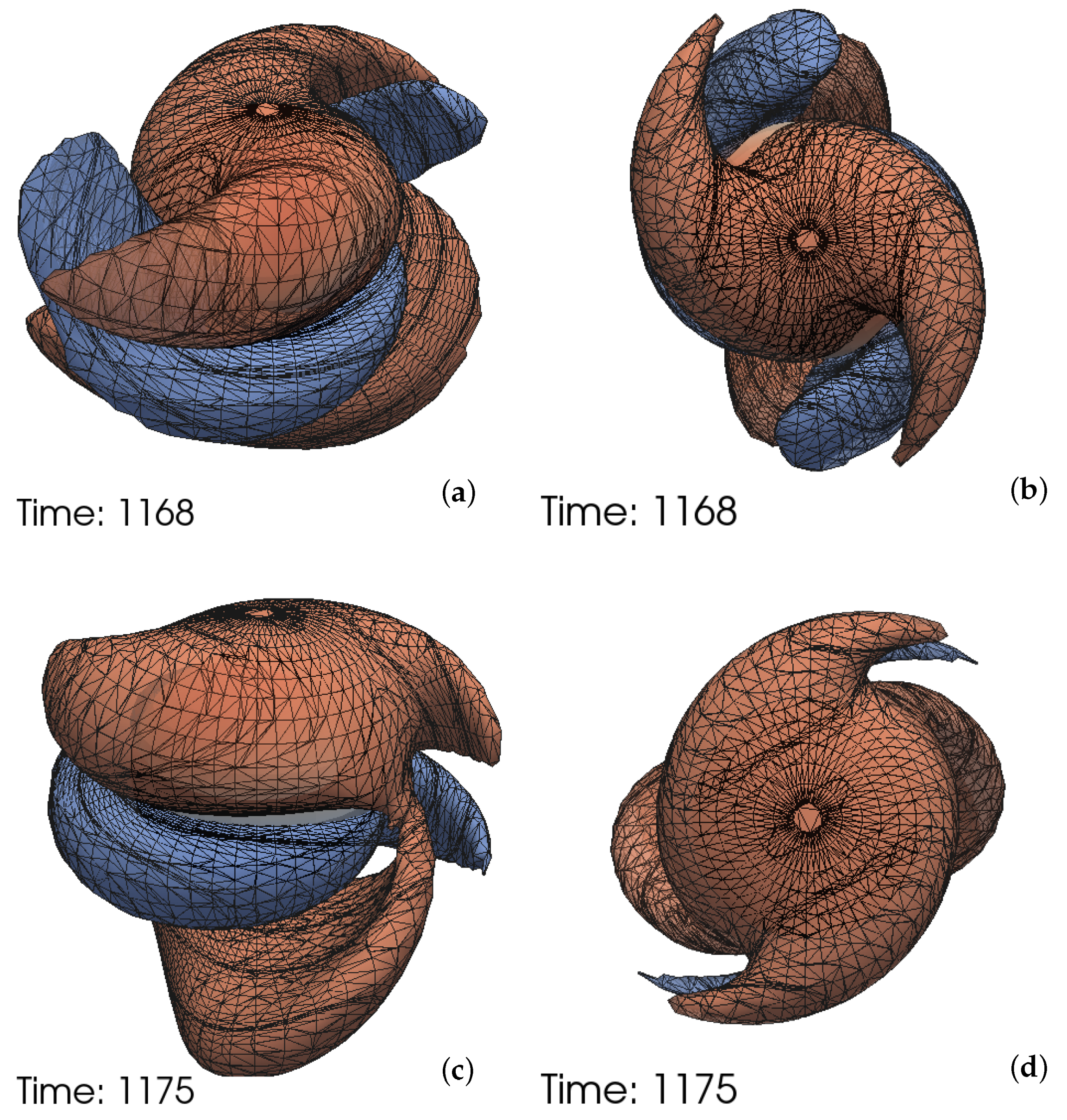
We now plot the time evolution (during the merger phase) of the opposite vorticity contours for the SK simulation in the top two rows of
Figure 3, and see an increase of alignment over time, suggesting a decreasing current quadrupole moment. We also note that the blue spiraling arms in
Figure 3a slice through the orbital plane, while their counterparts in
Figure 3c do not behave in the same way. Furthermore, the blue arms are larger in spatial extent initially, but reduce to be of similar sizes as the red arms later. These features are also consistent with a declining current quadrupole contribution. For comparison, we also plot in the bottom row of
Figure 3, the contours for the AA simulation at the same time delay from merger as in
Figure 3a,b, where as the current quadrupole moment vanishes according to Equation (
4), the contours are already exactly aligned.
3. Avenue for the Exit of the Current Quadrupole
If we hold spin magnitude
S constant, and keep spin directions tangential to the orbital plane in a
-symmetry configuration, then a comparison between Equation (
5) and Equations (
6)–(
8) suggests that as
R decreases, the relative strength of
as compared to
should increase. Using the values for
M and
S in
Table 1, we find that
and
should become similar in magnitude when
, or around merger time. Furthermore, if
for the
r range we are interested in (e.g., the range plotted in
Figure 3), then the first terms dominate in Equations (
9) and (
11), and the ratio of
field strength as generated by
to that generated by
is multiplied by a factor of
on top of the strength ratio between
and
. On the other hand, when
, all the terms in Equations (
9) and (
11) contribute, so the additional factor is around 1 because all the terms introduce an
factor. In other words, the current quadrupole is either more effective or equally effective at generating the vortex field as compared to the mass quadrupole. This conclusion should remain true in a strong gravitational field, as
can be seen as the primary field generated by
, while only a secondary field for
that is induced by the time variation of
(see Section VI C and Section VI D 1 of Reference [
15] for further discussions and examples). Consequently, as the absolute magnitude of
catches up to or even overtakes that of
during the merger phase, we should not see its influence in vorticity decline in the fashion of
Figure 3. Therefore, the current quadrupole must somehow diminish during the merger phase. It would vanish if the equal and opposite spins of the two individual black holes simply annihilate each other, but this does not explain why spins annihilate faster than the two masses merge (i.e., why the current quadrupole declines faster than the mass quadrupole). In other words, we need the current quadrupole to reduce faster than the signature of the individual black holes disappears.
Such a scenario is possible if the individual spins experience a re-orientation into configurations that produce near-vanishing
, even as the spins themselves are still non-vanishing. This can be achieved if the spins move to become nearly aligned with each other, which according to Equation (
4) would result in a nearly vanishing
.
Above, we have used the term “individual spins” in a generalized sense. Even before merger, the spins of the individual black holes are really reflections of the spacetime dynamics outside of these holes, as the characteristic modes for the Einstein equation are strictly outgoing at the apparent horizons (which are inside the event horizons). The merger would not instantaneously remove the near-zone dynamics that were underlying the individual spins, so one may regard the continuation of such dynamics as a kind of remnant spin (the word “remnant” will be omitted frequently for brevity). In the tendex and vortex language, one may say that these remnant spins are the vorticity and tendicity of the spacetime that were associated with the spins before merger, but would not instantly dissipate upon the formation of the common apparent horizon. Similarly, the tendicity and the vorticity of the spacetime that were associated with the orbital motion of the individual black holes before merger continue to evolve post-merger, and provide a remnant orbital motion. We note that the remnant spins considered here belong to the defunct individual black holes, and are not the spin of the remnant black hole.
Due to the lack of analytical descriptions for highly dynamic regimes, we will rely on the available perturbative expressions to aid our qualitative arguments in the rest of this section. Although we are likely pushing these expressions beyond their reasonable range of validity, we will only be interested in the qualitative features of the spacetime they expose, and not their quantitative accuracy.
In order to achieve alignment, it is required that the spins be lifted out of the orbital plane, either through spin–orbit coupling or spin–spin coupling, because the
-symmetry forbids the spins from being aligned when they are confined to the orbital plane. The spin–orbit coupling is given by the leading order PN expression [
25,
26,
27,
28]:
in the center-of-mass frame, where
is the orbital angular momentum at the Newtonian order:
with
being the reduced mass and
, and also
R being the magnitude of
. For the post-merger context, we will instead take
to be
minus the remnant individual spins. We note that the
in Equation (
15) cannot point out of the orbital plane and will only generate spin precession within it.
The spin–spin coupling, on the other hand, can create a torque pointing out of the orbital plane. The leading order expression for spin–spin coupling is given by [
25,
26,
27,
28]:
in the center-of-mass frame, and
is defined as
. For the SK configuration,
when the spins are in the orbital plane, as they must be anti-parallel by
-symmetry, but
is not required to be transverse (especially when the spins are not locked to the orbital motion), so
and there is a
in the direction orthogonal to the orbital plane. Normally, this direction is not constant over an orbital cycle for a pair of spins not locked to the orbital motion, so the spin–spin coupling effect does not accumulate significantly during early inspiral, but as the merger phase will not take up a whole cycle, we need not worry about cancellations. On the other hand, the directions of
and
are the same, so as desired, the spins for our SK configuration either both move upwards (more aligned with
) or both move downwards (more anti-aligned with
), retaining the
-symmetry.
According to Equation (
17), the spins do not need to move towards spin–spin alignment. In fact, the
-symmetry enforces
, so unless
, the spins would never be aligned. The situation would change however if we include the radiation reaction. Because gravitational waves drain dynamical energy, radiation reaction should push the spin orientations towards an energetically favorable equilibrium configuration, where the spin precession due to both spin–spin and spin–orbit coupling ceases. From Equation (
15), it is clear that the spin–orbit induced precession would shut off only when
and
are orthogonal to the orbital plane, or in other words are collinear with
. Furthermore, Equation (
17) shows that the spin–spin coupling generated spin precession also stops for such configurations. In addition, when the spins are either both aligned or both anti-aligned with
(henceforth referred to as spin–
alignment or anti-alignment), the current quadrupole will vanish.
For this postulate to work, a necessary condition is that the spin–
alignment or anti-alignment configuration should correspond to a local minimum in energy. To this end, we note that the potential energy associated with the spin–spin interaction at leading order is given by References [
25,
26,
27,
28] as:
while the potential for the spin–orbit coupling is [
25,
26,
27,
28]:
The absolute minimum of
is achieved when
and
are anti-parallel and collinear with
, as the second term in the square bracket of Equation (
18) favors anti-parallel orientations and dominates over the parallel-orientation favoring first term, due to its extra factor of 3. This is also an equilibrium configuration for Equation (
17), but does not lead to a small current quadrupole moment, as shown by Equation (
8).
For the spin–
alignment or anti-alignment equilibrium configurations that we are interested in, we have
or
, and
, with
being the angle
spans with
and
the angle between
and the projection of
into the plane orthogonal to
. The angles
and
are defined similarly for
. It is easy to verify that all first derivatives of
against the angles vanish for these configurations, so they are indeed critical/equilibrium points. However, the eigenvalues of the Hessian are
and not all positive, so they are not (local) minima of the potential energy. When we add in the potential
, which achieves its absolute minimum at the spin–
anti-alignment configuration, the eigenvalues of the Hessian (of
) for this configuration become:
where we have taken
and
to simplify expressions. For our
simulations, and using the Newtonian expression for
, spin–
anti-alignment configuration is a local minimum as long as
M. The spin–
alignment configuration, on the other hand, has eigenvalues:
and is therefore not a local minimum unless
is sufficiently negative. When we add in the next-to-leading-order PN expressions for
[
29,
30,
31,
32,
33], we acquire extra multiplicative factors onto
that can reverse the sign of the effective
at small
r, and make spin–
alignment configuration a local minimum (effective
in
is reversed, but
is not, so anti-alignment with the effective
now results in an alignment with
). The
that includes both leading and next-to-leading order PN contributions can be deduced from the spin precession equation (Equations 61-64 in Reference [
31]; also note that post-Newtonian derivations with spin all rely on some spin supplementary conditions, which is an added ambiguity that we inherit):
in a general frame, where we can regard
as an effective
for
, and
’s contribution to
is
. The quantities appearing in Equation (
22) are:
and more importantly:
with
and
. Note
is in the opposite direction to particle 2’s orbital angular momentum, so the
term in Equation (
25) could reverse the direction of the effective
when
R is small.
Strictly speaking, the difference between
and
can become substantial near merger, and since it is the latter that we extract from simulations, Equations (
22) and (
25) can not provide useful simple intuitions regarding the spin dynamics. Indeed, since radiation reaction becomes significant in that regime, the quantitative correctness of these conservative expressions is not guaranteed in the first place (precise analytical expressions are not available for the merger phase, which is one of the reasons why numerical simulations are indispensable). The reason why we evoke these next-to-leading order expressions at all is merely because they demonstrate the qualitative behaviour that the effective
can have a sign reversal, making alignment a viable local energy minimum. Throwing away the crutch of perturbative expressions, we really only need the qualitative statements, that the spin–
near-alignment or near-anti-alignment configurations are energetically favorable for the spin–orbit coupling, and that mechanisms like the spin–spin coupling exist that can lift the spins out of the orbital plane (see e.g., [
34,
35] and Figure 5 of [
36] for other studies of this effect in the superkick context), to remain true in the strong field regime. The perturbative expressions have hinted that it may be possible to meet these requirements, but strong field expressions are needed for quantitative assessments.
Another condition for our postulate to work is that the remnant spin dynamics should be efficient radiators during the merger phase, such that the spins experience a significant reaction. In contrast, when modeling early inspiral, the radiation reaction felt by the spins is usually neglected [
28,
37] (see in particular Equation 17 of [
37], showing that the radiation reaction torque produces a higher order effect than the conservative spin precession effects). If we plot the distribution of
near the common apparent horizon, we should see a close association between the high intensity regions of
and entities that can be interpreted as representing the remnant spins. To verify this, we adopt the quasi-Kinnersley tetrad described in References [
38,
39,
40,
41,
42,
43]. Our particular version of the tetrad follows Reference [
38] and suffers from some numerical noise because of the third derivative of the metric required for its construction. However, because we are now examining the region very close to the remnant black hole, the mixing of
into
under a simple simulation–coordinate-based tetrad will overwhelm the interesting features. The quasi-Kinnersley tetrad avoids this problem by correctly identifying the gravitational wave propagation direction [
38]. Specifically, the tetrad bases correspond directly to the super-Poynting vector, so that the
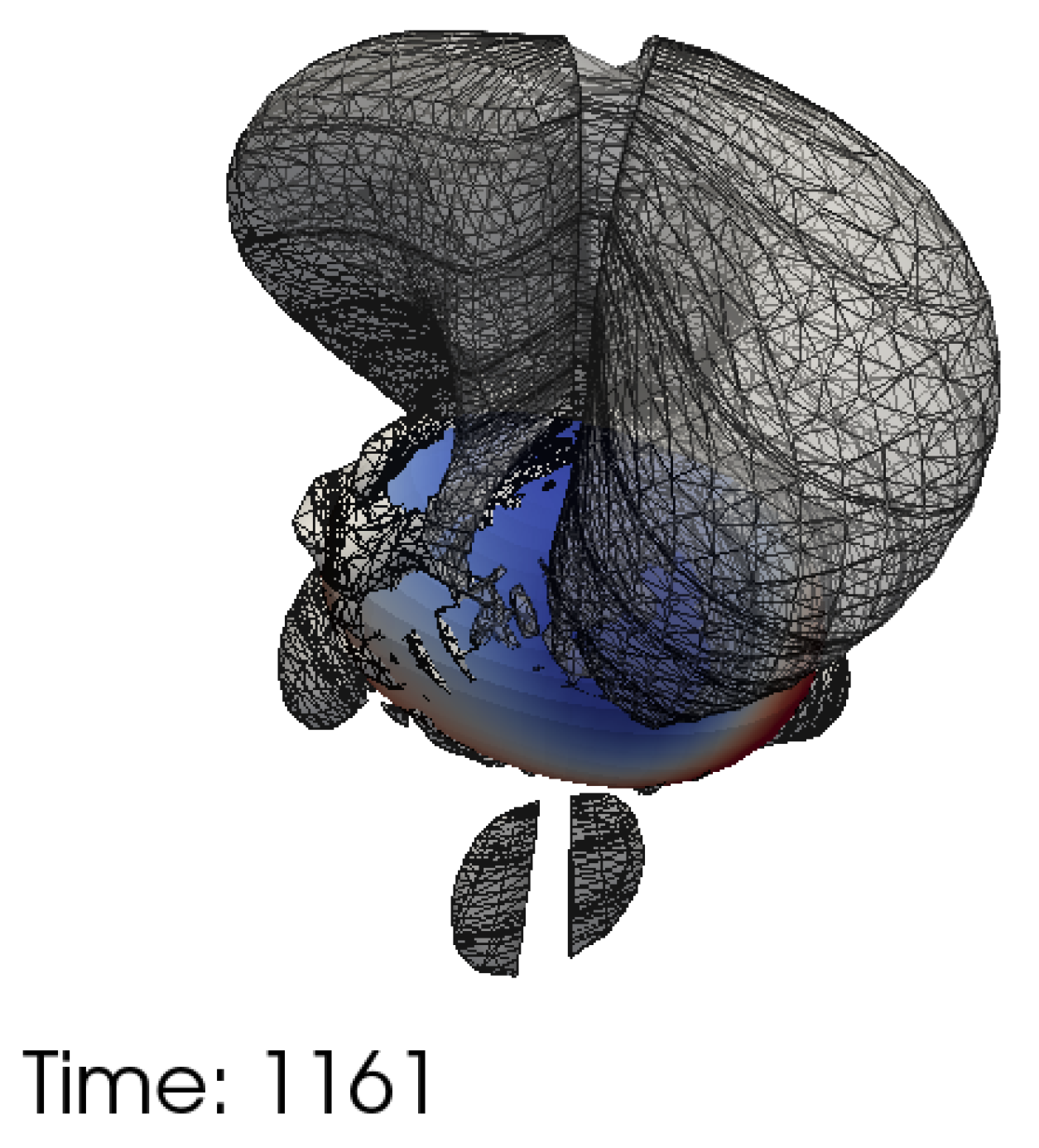
extracted under this tetrad retains a simple relationship with the energy flux even in the near zone. In
Figure 4, we plot a large absolute value, and thus close to the radiating source, contour of
. It is clear that this contour attaches to certain blue horizon vorticity patches (contours of even higher
are seen to be confined to regions closer to these patches), which we will now show (in
Section 4) to be direct manifestations of the remnant spins.
4. Visualizing the Remnant Spins
One possible way to visualize the (remnant) spins directly is through the horizon vorticity
. This quantity is closely related to the spin measurement expressed as an integral over the horizon [
44,
45,
46], namely [
23]:
where
is the area element on the horizon, and for the event horizons,
is
plus some spin coefficient corrections that vanish in a stationary limit (see References [
7,
23]). We will use the apparent horizons in this paper, which coincide with the event horizons in the stationary limit [
47], but are not teleological and therefore more widely utilized in numerical simulations. The quantity
in Equation (
26) is determined by an eigenvalue problem on the horizon, and is essentially an
spherical harmonic [
48]. In other words, the spin is given by the dipole part of the horizon vorticity
. For example, during early inspiral, the
pattern on each individual horizon is dominated by the spin of that black hole, forming a dipolar shape like those seen for the Kerr black holes in Reference [
23]. This is shown in
Figure 5a, and can be used to identify the spin directions.
Close to and past merger, aside from the overall
harmonic-weighted integral in Equation (
26), there are many interesting finer details that can be seen from the
plots for our various simulations shown in
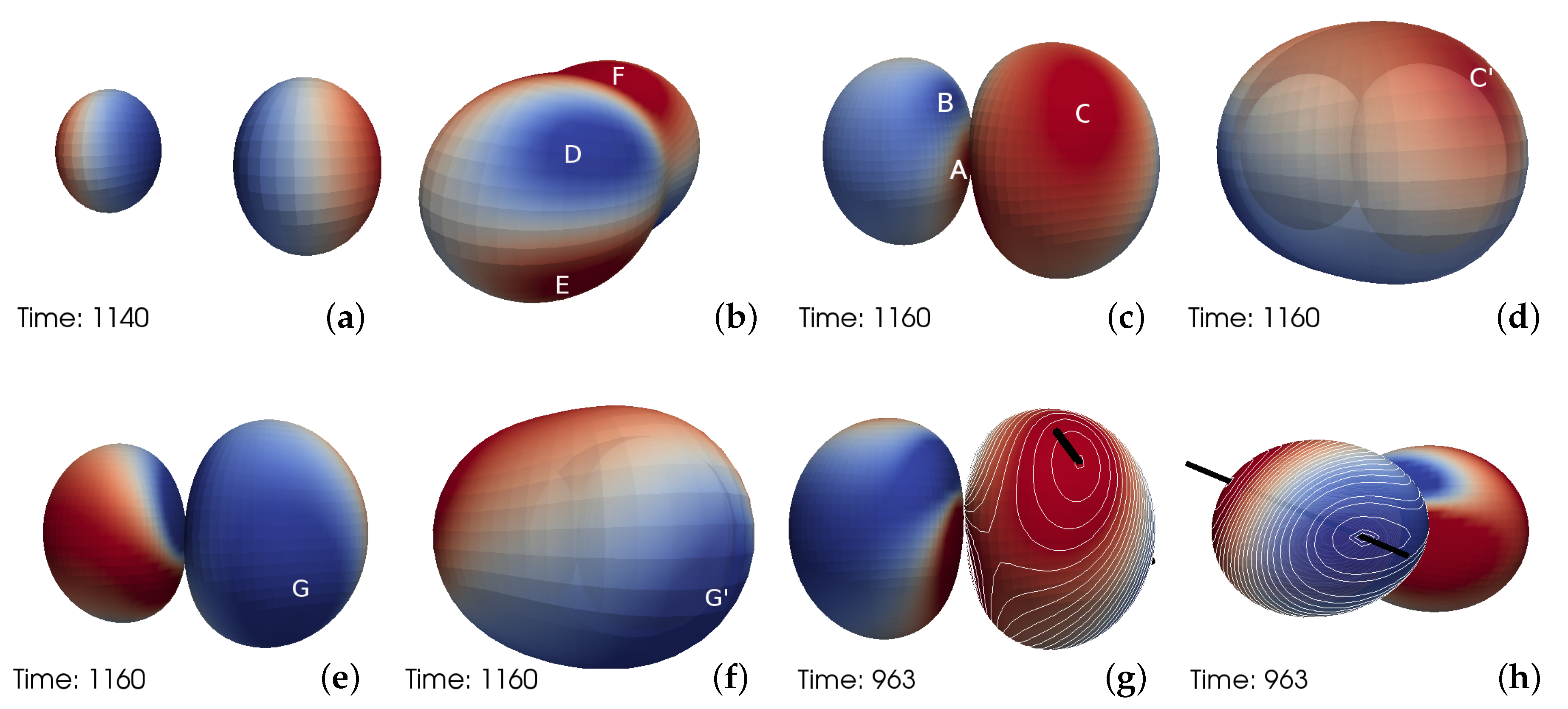
Figure 5. The panels (c)–(d), (e)–(f) and (g)–(h) of this figure depict the horizon vorticity patterns for the SK, SK- and SK⊥ simulations, respectively, while panel (b) shows the pattern for the AA simulation. The panels (b), (d) and (f) of
Figure 5 show the common apparent horizon, while the rest of the panels are for the two individual horizons. At the end of the inspiral stage, the horizon vorticity picks up visible new patches (e.g.,
A and
B in
Figure 5c for the SK simulation) that are absent during the inspiral phase, while the spin contributions are also present e.g., patch
C and a blue patch at the back that is blocked from view in
Figure 5c).
Post-merger, the horizon vorticity for the SK simulation is shown in
Figure 5d, where in addition to a dipolar contribution from the spin of the remnant black hole (similar to the
F patch in
Figure 5b for the AA simulation), there are also visible patches that can be interpreted as the continuation of the pre-merger spin patches. For example, the region
in
Figure 5d corresponds to patch
C in
Figure 5c, while the patches
D and
E in
Figure 5b correspond to the continuation of the pre-merger individual spins in the AA simulation that were anti-aligned with
. Such finer details in
on the common apparent horizon thus provide us with a more concrete manifestation of the abstract remnant spins discussed earlier.
We can now use the spin patches to track the pre- and post-merger (remnant) spin dynamics. First of all, we note that the SK- simulation is the same as the SK simulation aside from a reversal of the individual spins. Since Equation (
17) is invariant under
and
, we should see the spins lifting up into the same side of the orbital plane for these two simulations
1. A comparison between
Figure 5c–f confirms this expectation, and provides us with some confidence that the spin–spin coupling is indeed responsible for generating the
and
components at merger.
Using the numerical values for the spins (measured with Equation (
26) on each individual apparent horizon) and the numerical trajectories of the black holes in the simulation coordinates, we can further make a prediction for the
z components of the spins by integrating Equations (
15) and (
17). Namely, we calculate the
values at a dense collection of times for one of the spins according to lEquations (
15) and (
17), using the numerically measured
,
and
, before adding these
increments up into a predicted history for
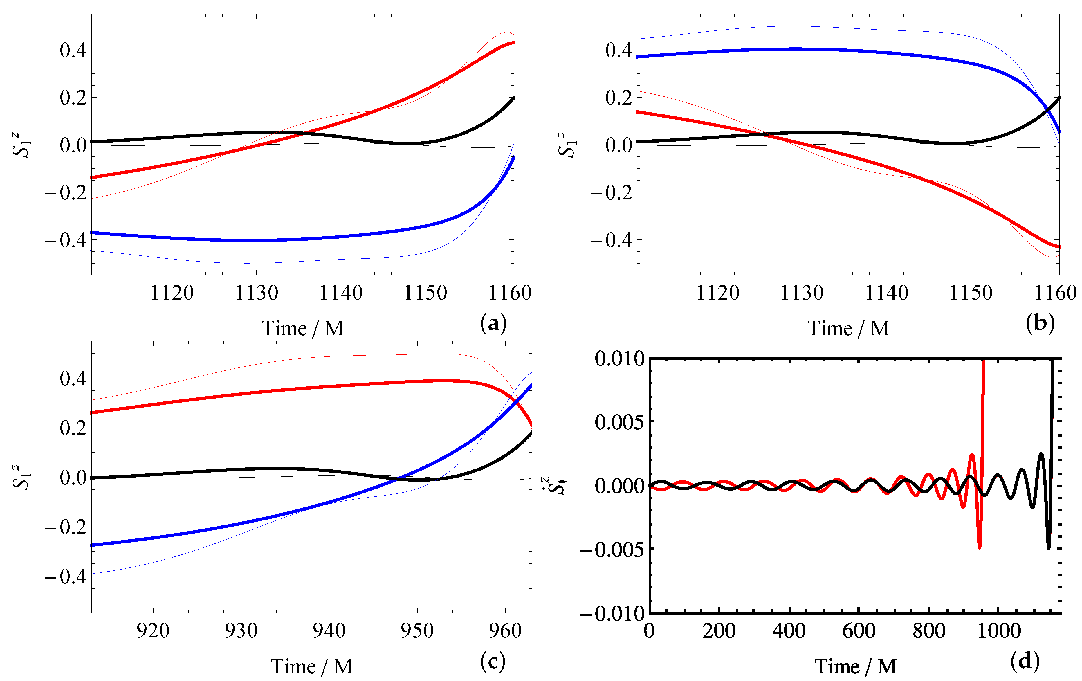
. The results are shown in
Figure 6. We see a steep rise of
for the SK, SK- and SK⊥ simulations towards merger, matching what is seen in the
spin patch. In particular, the prediction is for a dimensionless spin with
just before the merger for all three simulations, which translates into an angle of
that
spans with the orbital plane. Taking the SK⊥ simulation for example, the line connecting the centers of the +ve
and −ve
spin patches for this simulation (see
Figure 5g,h) spans an angle of
with the orbital plane, which is fairly close to the prediction. The closeness between these two numbers is somewhat surprising, in that the simulation gauge is not the same as the harmonic gauge used for the PN calculations, and that we are operating in a regime close to merger. To further test the quality of the PN prediction, we produce the predicted histories for
and
using the same prescription, and compare them to their numerically computed counterparts in
Figure 6, which also show general agreement.
The situation is different when we compare the predicted and the numerically computed
, as the latter lacks the steep rise just before merger that is also seen in spin patches. To understand this, recall that the numerical spin values are calculated as integral Equation (
26). Such an integration over the entire horizon does not distinguish the spin patches like
C and
G in
Figure 5c,e from the mass quadrupole induced patches
A and
B as in
Figure 5c. As the mass quadrupole patches on each apparent horizon resembles a spin pointing in the
direction at merger time (see
Figure 5c,e,g,h), the numerical spin measurement
according to Equation (
26) could be negative even when the post-Newtonian equivalent spin is positive. On the other hand, the measurements on
and
are less affected by this contamination. Furthermore, it is required that the first derivative of the scalar
in Equation (
26) should be a rotation generating approximate Killing vector [
49,
50,
51,
52], which may not be applicable when we approach the highly non-stationary merger phase.
One interesting feature we have seen with our simulations is that at the merger, the spins seem to have been preferentially lifted out of the orbital plane towards the spin–
alignment side (see
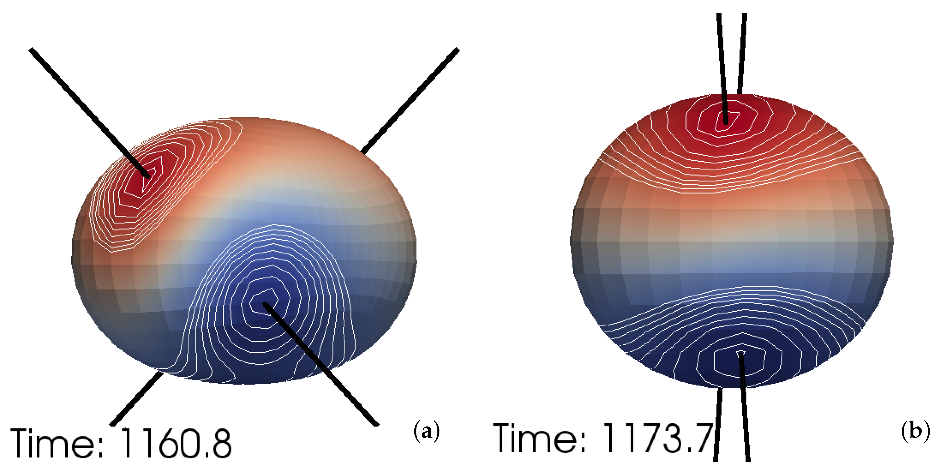
Figure 6d). This trend also continues post-merger, as shown in
Figure 7 for the SK simulation (similar behavior is seen for SK- and SK⊥), until a spin–
near-alignment is achieved, in agreement with our proposal in
Section 3. The SK⊥ simulation is particularly interesting in that its initial spin orientations are chosen such that if the black holes merge at exactly the same orbital configuration as the SK and SK- cases, we would have
at merger according to Equation (
17). Instead, the black holes merge with
(see
Figure 5g,h and
Figure 6c,d) at an earlier time. Therefore, based on our small sample of simulations, there appears to be a preference towards spin–
alignment at merger, which is not reversed post-merger. The exceptional case is the AA simulation, where the spins remain anti-aligned with
throughout the inspiral and merger phases, perhaps because the spins are stuck in a (possibly unstable) equilibrium configuration.
One possible explanation for the preference at merger time is provided by the spins’ influence on the orbital motion, through the extra acceleration [
25,
26,
27,
28,
53,
54,
55]:
In Equation (
27), we have only shown the spin–spin contribution, as we are interested in the beginning of the final ascent of
and
, and the spin–orbit contribution is small for our
-symmetric simulations when
and
are still small (i.e.,
). It is plausible that the BBH coalescence progresses quickly towards merger when
(radially pulling the black holes closer) and
(slowing down the transverse orbital motion of the black holes), such that the instantaneous impact parameter is altered in the direction conducive to merger. We note that only the second and third terms in the square bracket of Equation (
27) contribute to
, and these two terms have the same value in our
context. Therefore we have:
Comparing Equation (
28) with Equation (
17), we arrive at:
so that regions of
always correspond to
, and there would subsequently be a preference for spin–
alignment at merger.
5. Discussion
We note that an observation in this paper may help achieve a consistency between the QNM frequencies. First recall that an electric/magnetic parity quasinormal mode is defined to be one whose corresponding metric perturbation has the parity matching the sign of
/
. Because the
/
field has the opposite/same parity to the underlying metric perturbations [
22], the mass/current quadrupole would then excite the electric/magnetic parity
QNMs (see also Reference [
56], as well as Reference [
22] for discussions on the similarities between the mass/current quadrupole generated
and
fields and those associated with the electric/magnetic parity QNMs). The parity properties of the various quantities are summarized in
Table 2.
The electric and magnetic parity QNMs are degenerate in that they share the same complex frequency (see e.g., Section IC3 of Reference [
22] and Section VB1 of Reference [
56]). This has an interesting consequence, as was noted by Reference [
56] when motivating spin-locking in the superkick configurations. Namely, when QNMs of both parities are present, the current quadrupole should evolve at the same frequency as the mass quadrupole at the end of merger (just before the onset of the QNM ringdown phase). For the superkick configurations, because the mass quadrupole evolves at twice the orbital frequency, while the current quadrupole’s frequency is essentially a sum of the orbital and the spin precession frequencies, this further implies that the spin precession frequency must lock onto the orbital frequency [
56].
A robust mechanism must be present for this locking to occur. A calculation using the leading order PN spin–orbit coupling expression (
15) for a
-symmetric superkick configuration yields [
8,
56]:
where
is the spin precession frequency. Therefore, as the black holes move closer to each other,
can approach
and equalize with it [
8]. However, this equality is broken again when
reduces further. So instead of locking, we have only a momentary coincidence. Another mechanism for locking is proposed by Reference [
56], which considers geodetic precession in black hole perturbation theory. This alternative provides a stronger precession:
but is otherwise similar to the leading order PN spin–orbit coupling result. Without invoking further dynamics, one would then be forced to make the inference that the BBH QNM ringdown begins, and that the spacetime dynamics that can be construed as two individual black holes approaching each other, ceases, precisely at the
that gives
. Note that Equations (
30) and (
31) do not depend on the magnitude of the spins, so infinitesimal spins would appear to still play a vital role in the transition into the QNM ringdown phase. So additional dynamics are likely involved. For example, if the magnetic parity QNMs are completely absent, so that their frequencies become irrelevant, then the consistency would be achieved by default. Perhaps more interestingly, as discussed in relation to the next-to-leading-order PN corrections to
in
Section 3, the energetically favorable orientation of the spins have a frame-dependent offset from the directions of
. As this offset can evolve at the frequency of
when the precession of
is locked onto the orbital motion, we could in principle have a self-consistent sustained locking (as opposed to a momentary coincidence) scenario if the spins are kept in these orientations by, for example, the same dynamics that drove them there in the first place. In other words, the mechanism responsible for the decline of the current quadrupole moment may also be responsible for locking its frequency to the desired value. In this case, the magnetic parity QNMs will not need to vanish in the ringdown waveform. However, we are operating in a regime where the PN expressions are not expected to remain fully valid. To see whether similar effects are actually present in a strong field and fast motion setting, we plan to carry out further studies at a later date.
Finally, we note that in this paper, we have intentionally neglected to discuss gravitational waveforms, even though the wave modes are obviously quite directly connected to the multipole moments discussed here (see e.g., Reference [
57] for an example discussing the current quadrupole specifically). The reason is that while the multipolar evolutions investigated in the paper are concentrated into the merger phase, there is a regridding (bringing in with it some associated gauge dynamics) happening at the merger within the simulations carried out in this study, so the minute features seen in the waveform could possibly have been numerical in nature instead, or contain a nontrivial distortion of the real physics. More specifically, the waveform, as a spherical harmonic decomposition mode of the
component of the Weyl curvature tensor, is sensitively dependent on the coordinate choice both locally and globally. Locally, the dependence comes in via the fixing of the coordinate tetrad (physically corresponding to fixing the orientation, velocity, etc. of a gravitational-wave detector; a local coordinate transformation will change the tetrad and alter what content of the Weyl tensor is called
). The regridding gauge wave will shake the “virtual detector” in the numerical simulation in unphysical ways, resulting in it registering spurious oscillations due to this shaking and not the actual spacetime rippling. Furthermore, the waveforms are presented as only one or very few modes in the spherical harmonic decomposition (this projection already makes the effects of the spin dynamics difficult to decipher since any projection necessarily mix many different influences), but the definition of the harmonics depends on the global coordinates. The author had not been able to properly remove the effects of the gauge dynamics in the highly nonlinear merger regime, and thus does not feel confident making any firm assertions/connections. Instead, our study here had intentionally avoided doing any projections (the price we pay is that the time-varying three dimensional data then cannot be easily condensed into time series of numbers and our discussions are qualitative), and used the eigenvalues of spatial curvature tensors (tendexes and vortexes), which although are still dependent on how the spatial slicing is done, are invariant under spatial triad changes. Nevertheless, given the explosive growth of gravitational wave astronomy, including actual data, it is worth investigating whether the qualitative conclusions made in this paper can be extracted out of enhanced observational data, e.g., by stacking the data of multiple events.


