A Modified Dynamical Model of Cosmology I Theory

Abstract

Wheeler (1964) had formulated Mach’s principle as the boundary condition for general relativistic field equations. Here, we use this idea and develop a modified dynamical model of cosmology based on imposing Neumann boundary condition on cosmological perturbation equations. Then, it is shown that a new term appears in the equation of motion, which leads to a modified Poisson equation. In addition, a modified Hubble parameter is derived due to the presence of the new term. Moreover, it is proved that, without a cosmological constant, such a model has a late time-accelerated expansion with an equation of state converging to $w<-1$. Also, the luminosity distance in the present model is shown to differ from that of the $\Lambda CDM$ model at high redshifts. Furthermore, it is found that the adiabatic sound speed squared is positive in radiation-dominated era and then converges to zero at later times. Theoretical implications of the Neumann boundary condition have been discussed, and it is shown that, by fixing the value of the conjugate momentum (under certain conditions), one could derive a similar version of modified dynamics. In a future work, we will confine the free parameters of the Neumann model based on hype Ia Supernovae, Hubble parameter data, and the age of the oldest stars.

1. Introduction

The question of the existence of dark matter and dark energy and their implications at different cosmic scales has been the dominant subject of the contemporary cosmology. The main argument in favor of these two components is that their presence would solve some otherwise baffling discrepancies between observations and predictions of general relativity (GR). See References [1,2]. These predictions are mostly based on the zero- and first-order perturbation equations of GR field equations. See References [3,4,5,6,7] for reviews on perturbation method in general relativity.

For example, the presence of the dark matter particles could explain most notably, among other phenomena, the growth of structures in the universe, the stability of gravitating systems, the rotation curves of spiral galaxies, and the missing mass problem in gravitational lensing. See References [1,8,9] for excellent reviews on the essence of these problems. However, it should be noted that, despite tremendous efforts to detect the most popular candidates of dark matter, such as sterile neutrinos, WIMPs (weakly interacting massive particles), and axions, a conclusive evidence for the detection has not yet been reported [10].

On the other hand, the existence of the dark energy is presumed to explain the large-scale structure and evolution of the cosmos [2,11]. The main concerns here are accelerated expansion of the universe (proved by References [12,13] based on supernova observations), baryon acoustic oscillations, temperature anisotropies in the cosmic microwave background (CMB), and the age of the universe. See Reference [11] for a thorough review on theoretical implications and observational evidence of dark energy. Also, see Reference [14], which reviews dark energy models from different perspectives.

To solve GR field equations, the initial/boundary conditions are usually considered to be trivial. See Referece [1] pages 361–363 for a discussion on this issue. The question of initial/boundary condition in GR is closely related to the problem of the boundary term in GR action. At least from a mathematical point of view, it is well understood that, to derive the Einstein equations, one has to add a surface term to the Einstein–Hilbert action [15]. This ensures a well-posed action, meaning that the imposed boundary condition on the action is compatible with the derived field equations. The main issue in adding a surface term to the Einstein–Hilbert action is the quantity which should be fixed on the boundary. On the other hand, Wheeler’s [16] interpretation of Mach’s principle suggests that, in addition to the energy momentum tensor, one needs also to specify the boundary condition to derive the structure of spacetime. See also Reference [17] for a review on this idea. This view toward solving Einstein field equations is mostly based on the necessity of mathematical and physical well posedness of the theory rather than philosophical grounds of Mach principle, which are well discussed by Reference [18]. In fact, this interpretation of Mach’s principle is closely related to the Cauchy problem of GR [19,20]. There are various formulations of Mach’s principle in the literature. For example, Bondi and Samuel [21] distinguish eleven statements, Mach0 to Mach10, of Mach’s principle; however, Wheeler’s formulation is not included. We will discuss some of these statements below. Also, References [17,22] propose similar ideas to Wheeler’s in their attempt to find generally covariant integral formulation of GR.

In their work on the foundations of gravitational theories, Thorne, Lee, and Lightman [23] define boundary conditions as those laws which involve only confined variables. As these authors have illustrated, “if one augments the theory by cosmological demands that $\varphi$ and $\psi$ [the scalar potentials] go to zero at spatial infinity, those demands are boundary conditions”. We will discuss this particular case in the following.

Including boundary dynamics while solving GR field equations could lead to interesting results even at the quantum level [24,25]. For example, Park [26] considers the issue of “changing black hole mass through Hawking radiation” and finds that, by imposing Neumann boundary condition, one could solve the problem. See also a recent work by Witten [27], who shows that the usual Dirichlet boundary condition is indeed not elliptic. Thus, in general, this boundary condition does not provide a well-defined perturbation theory. On the other hand, Witten shows that conformal boundary conditions always lead to a sensible perturbation expansion. Therefore, when we solve GR field equations, it is important to check different possibilities of boundary conditions both for the sake of mathematical well posedness of the model and its compatibility with physical expectations.

In this work, we will impose Neumann boundary condition (B.C.) on GR perturbation equations. Also, the modifications in trajectories of massive and massless particles are discussed. The new term in the equation of motion of this model is found to be proportional to $c{H}_0=6.59\times {10}^{-10}$ m/s${}^2$ in which c is the speed of light and $H_0$ is the Hubble constant [28,29]. This parameter is also known as the de Sitter scale of acceleration [30,31]. Thus, the model is essentially a modified dynamical (MOD) model which, in many features at galactic scales, shows some similarities with Milgrom’s proposal [32,33,34] known as MOND (modified Newtonian dynamics). See Reference [35] for a review on MOND. Some particular aspects of galactic dynamics, such as observed regularities in the properties of dwarf galaxies [36,37], are illustrated within the context of MOND quite better than the cold dark matter ( CDM ) paradigm. The main implication of the appearance of such an acceleration scale in the equation of motion is that, probably, the physics of the local universe might be affected by the global expansion of the cosmos [8]. Many works try to explain the phenomenological success of MOND by deriving particular versions of it from action principle. For example, a recent article by Vagnozzi [38] demonstrates that MOND can be recovered in the low-energy limit of mimetic gravity. The acceleration scale in this approach changes with length scale in such a way that the model is able to explain dark matter both on galactic and cluster scales.

Using our new modified Poisson equation and the averaging procedure of backreaction cosmology [39,40,41,42], in Section 3, a governing modified Hubble parameter of the present model is derived. Then, in Section 4, the main cosmic implications of the new model is surveyed. Among others, we have derived the evolution of the scale factor, Hubble parameter, deceleration parameter, equation of state, and adiabatic sound speed. In a future work, we will present a data analysis of the model based on Supernovae Type Ia (SNIa) and Hubble parameter data (Shenavar and Javidan, in preparation). The basic parameters of the theory could be derived from such analysis.

Some related explanations and elaborations are postponed to the Discussions section and in the appendices. In Section 5.1, we search for the implications of Neumann B.C. from an action-principle point of view. Prior works by Maldacena [43] and by Anastasiou and Olea [44], who propose the equivalence of Einstein and conformal gravity under Neumann B.C., are discussed. Also, we consider the works of References [15,45] that prove the existence of a well-posed Neumann boundary condition. The surface term introduced by References [15,45] has the peculiarity that it vanishes in a four dimensional spacetime. In particular, we have shown that, by assuming some conditions on scalar potentials, our choice of Neumann B.C. in Section 2 could be derived based on the procedure that References [15,45] define. Discussions regarding the averaging problem and Mach’s priciple have been presented in the rest of Section 5. In addition, we have provided detailed analysis of the role of geometrodynamic clocks and EPS ( Ehlers, Pirani and Schild [46]) theorem in Appendix B. Moreover, a discussion on the dimensional analysis of the model is presented in Appendix C. Furthermore, we report a similar semi-Newtonian model in Appendix D, which is built based on some well-motivated theoretical and observational assumptions.

In Reference [28], the existence of a cosmological constant $\Lambda$ was assumed to ensure the existence of a late time epoch of accelerated expansion. Here, however, the $\Lambda$ term is abandoned and we will show that the modified Hubble parameter derived from imposing a Neumann B.C.—which includes a term proportional to H similar to Veneziano ghost of QCD (Quantum Chromodynamics) [47,48]—would naturally lead to an accelerated expansion of the universe with an equation of state parameter approaching to $w<-1$ at later cosmic times. The Neumann model proposes a unification of dark matter and dark energy. Such models have been proposed before. For example, one could see the generalized Chaplygin gas [49], k-essence [50], and Bose–Einstein condensation model [51]. We will compare the results of the Neumann model with these models and MOG (modified gravity of Moffat [52]), which is a model of dark matter (plus $\Lambda$ as dark energy), in the following.

2. A New Model of Modified Dynamics

In this section, we use the variational method of Weinberg [7], chapter 5, to find the Taylor expansion of GR field equations. One may also see References [3,4,5,6] for precise descriptions of the general perturbation theory of Einstein field equations. To do so, we will first fix the gauge condition to eliminate the spurious gauge degrees of freedom. Then, we will impose the boundary condition on the remaining physical fields.

2.1. Fixing the Gauge and the Boundary Conditions

We assume a flat Friedmann–Lemaitre–Robertson–Walker (FLRW) background metric disturbed by the perturbation of the local universe $h_{\mu \nu }$. Under spatial rotation, the symmetric perturbation metric could be decomposed into a scalar $h_{00}$, a three-vector $h_{0i}$, and a symmetric two-index spacial tensor $h_{ij}$. The tensor $h_{ij}$ could itself be decomposed to a trace part and a trace-free part. The resulting field equations, as Reference [7] has reported in chapter 5, would be very complicated. Also, they would contain some unphysical scalar and tensor modes which are correlated with the gauge freedom of the field equations.

This gauge problem could in principle be solved by working with gauge invariant quantities; however, in this way, the issue of imposing a new boundary condition on field equations would not be physically evident. Another method to eliminate the gauge degrees of freedom is by fixing the gauge which we use here. This process could be significantly simplified if the scalar, vector, and tensor modes of the perturbation metric are treated separately. Consider a general coordinate transformation

$$\begin{array}{c}\hfill x^{\mu }\to {x^{\prime }}^{\mu }=x^{\mu }+{\xi }^{\mu }\end{array}$$

(1)

in which ${\xi }^{\mu }$ is of the same order of the perturbation. To distinguish the behaviour of different modes under this transformation, we decompose the spatial part of ${\xi }^{\mu }$ as

$$\begin{array}{c}\hfill {\xi }_i={\partial }_i{\xi }^S+{\xi }_i^V\end{array}$$

(2)

with the condition that the ${\xi }_i^V$ is a divergenceless vector, i.e., ${\partial }_i{\xi }_i^V=0$. As Weinberg [7], pages 235–238, shows that the tensor quantities in perturbation metric and perturbation energy-momentum tensor are gauge invariant, there is no need to gauge-fix these modes. On the other hand, the vector ${\xi }_i^V$ could be chosen so that some vector degrees of freedom vanish. Lastly, to gauge-fix the scalar modes, there are various possibilities; however, here, we use the Newtonian gauge because, in this gauge, it is more convenient to adopt a new boundary condition. Of course, conversion to other gauges could be done as usual. In Newtonian gauge, two scalar degrees of freedom could be eliminated by choosing ${\xi }^S$ and ${\xi }_0$. Thus, the remaining scalars lead to the next metric (Weinberg [7] page 239)

$$\begin{array}{c}\hfill d{s}^2=-(1+2\Phi )d{t}^2+R^2(t)(1-2\Psi ){\delta }_{ij}d{x}^{i}d{x}^j\end{array}$$

(3)

in which $R(t)$ is the scale factor and the potentials $\Phi$ and $\Psi$ are functions of spacetime, i.e., $\Phi =\Phi (t,x,y,z)$ and $\Psi =\Psi (t,x,y,z)$. Our notation is very close to Weinberg’s [7], however, as a deviation from Weinberg’s notation, we keep $a(t)$ for the dimensionless scale factor $a(t)\equiv R(t)/R_0$ in the following.

One should note that the two scalar potentials are, in principle, distinct degrees of freedom. In fact, from a physical point of view, the potential $\Phi$ is a generalization of the Newtonian potential because it specifies the particle acceleration while the potential $\Psi$ is the 3-curvature perturbation of a constant-time surface. While many works consider the two potentials to be the same, the key assumption of this work is that these potentials could be essentially different.

The resulting field equations, as we will see below, would contain second-order spatial derivatives which certainly need boundary conditions to provide a unique solution. Indeed, by imposing a suitable boundary condition, as Wheeler’s interpretation of Mach’s principle demands, one could uniquely determine the solution to the field equations. The aim of the present work is to provide a new solution for the perturbation equations based on imposing Neumann boundary condition.

Using the metric in Equation (3), it is now straightforward to derive the local and background terms of Christoffel symbols, Riemann, Ricci, and Einstein tensors. These quantities have already been reported by many authors for the full perturbation metric (which includes vector and tensor terms in addition to scalar potentials) [3,4,6,7]. For the sake of brevity, here, we only report Christoffel terms and elements of Einstein tensor which will be needed in following.

The Christoffel symbols, up to first-order terms, are

$$\begin{array}{ccc}\hfill {\Gamma }_{00}^0& =& \dot{\Phi }\hfill \\ \hfill {\Gamma }_{00}^i& =& \frac{{\partial }_i\Phi }{R^2}\hfill \\ \hfill {\Gamma }_{i0}^0& =& {\partial }_i\Phi \hfill \\ \hfill {\Gamma }_{ij}^0& =& {\delta }_{ij}\left(R\dot{R}-(2R\dot{R}\Phi +\dot{\Psi })\right)\hfill \\ \hfill {\Gamma }_{j0}^i& =& {\delta }_{ij}\left(\frac{\dot{R}}{R}+\frac{1}{R^2}(2H\Psi -\dot{\Psi })\right)\hfill \\ \hfill {\Gamma }_{jk}^i& =& \frac{1}{R^2}\left({\delta }_{jk}{\partial }_i\Psi -{\delta }_{ij}{\partial }_k\Psi -{\delta }_{ik}{\partial }_j\Psi \right)\hfill \\ \hfill \end{array}$$

(4)

while the components of Einstein tensor are as follows

$$\begin{array}{ccc}\hfill G_0^0& =& -3{(\frac{\dot{R}}{R})}^2+\frac{2}{R^2}\left(3\Phi {\dot{R}}^2-{\nabla }^2\Psi +3R\dot{R}\dot{\Psi }\right)\hfill \\ \hfill G_0^i& =& \frac{2{\partial }_i}{R^3}\left(\dot{R}\Phi +R\dot{\Psi }\right)\hfill \\ \hfill G_j^i& =& \frac{{\partial }_i{\partial }_j}{R^2}(\Psi -\Phi )j\ne i\hfill \\ \hfill G_i^i& =& -\frac{{\dot{R}}^2+2R\ddot{R}}{R^2}+\frac{1}{R^2}(2{\dot{R}}^2\Phi +4R\ddot{R}\Phi +({\nabla }^2-{\partial }_i^2)(\Phi -\Psi )+2R\dot{R}\dot{\Phi }+6R\dot{R}\dot{\Psi }+2R^2\ddot{\Psi }).\hfill \\ \hfill \end{array}$$

(5)

All terms higher than the first order have been dropped in Equations (4) and (5).

On the other hand, the right hand side of the Einstein field equation, i.e., the energy-momentum tensor $T_{\mu \nu }$, could be decomposed to pure time-dependent zero-order terms $\rho$ and P and also spacetime-dependent first-order perturbations as follows

$$\begin{array}{ccc}\hfill T_0^0& =& -\rho -\delta \rho \hfill \end{array}$$

(6)

$$\begin{array}{ccc}\hfill T_0^i& =& -\frac{\rho +P}{R^2}\delta u_i\hfill \end{array}$$

(7)

$$\begin{array}{ccc}\hfill T_j^i& =& \left(P+\delta P\right){\delta }_{ij}+{\partial }_i{\partial }_j{\pi }^S\hfill \end{array}$$

(8)

where $\delta \rho =\delta \rho (t,x,y,z)$, $\delta P=\delta P(t,x,y,z)$, $\delta u_i=\delta u_i(t,x,y,z)$, and ${\pi }^S={\pi }^S(t,x,y,z)$ are respectively the local density, pressure, velocity, and scalar anisotropic perturbations [7]. This last term, i.e., ${\pi }^S$, displays the deviation from the perfect fluid model. In this work, the vector and tensor parts of the anisotropic stress tensor will be neglected. Also, for the sake of brevity, the dependency to spacetime parameters $(t,x,y,z)$ is not shown. It should be noted that the velocity perturbation could be decoupled into scalar and vector parts, i.e., $\delta u_i={\partial }_i\delta u+\delta u_i^V$; however, here, we only consider the scalar share in the velocity perturbation $\delta u$.

Now, one could use the energy-momentum conservation equation, i.e.,

$${\nabla }_{\mu }{T}^{\mu \nu }=0$$

to derive the next up-to first-order conditions

$$\begin{array}{cc}0=& \dot{\rho }+3\frac{\dot{R}}{R}(\rho +P)+\frac{(\rho +P)}{R^2}{\nabla }^2(\delta u)+3\frac{\dot{R}}{R}(\delta \rho +\delta P)-6\frac{\dot{R}}{R}(\rho +P)\Phi +\frac{\dot{R}}{R}{\nabla }^2{\pi }^S-2\Phi \dot{\rho }+\dot{\delta \rho }-3(\rho +P)\dot{\Psi }\hfill \\ 0=& {\partial }_i\left(3\frac{\dot{R}}{R}\delta u(\rho +P)+(\dot{\rho }+\dot{P})\delta u+\delta P+(\rho +P)\Phi +{\nabla }^2{\pi }^S+(\rho +P)\dot{\delta u}\right)\hfill \end{array}$$

(9)

which could also be derived, order by order, from Einstein field equations.

It is possible now to find the Einstein field equation, i.e.,

$$\begin{array}{c}\hfill G_{\nu }^{\mu }=\kappa T_{\nu }^{\mu }\end{array}$$

(10)

in which $\kappa =8\pi G$ is a constant, by using Equations (5) and (6). For example, by using ${}_j^i$ components of the Einstein equation, one could find

$$\begin{array}{c}\hfill {\partial }_i{\partial }_j\left(\Phi -\Psi +\kappa R^2{\pi }^S\right)=0\end{array}$$

(11)

which is reported in many classical literature on cosmic perturbation theory. See, for instance, Bardeen [3] and Mukhanov et al. [4]. Equation (11) manifests that the difference between tidal forces due to $\Phi$ and $\Psi$ is due to the anisotropic stress ${\pi }^S$. In particular, if ${\pi }^S=0$, then the tidal forces are equal ${\partial }_i{\partial }_j\Phi ={\partial }_i{\partial }_j\Psi$.

However, the field equations are at hand at this point, the appropriate boundary condition is yet to be imposed [16]. See Figure 1, which shows a typical gravitational source (here a galaxy) in a smooth background and its related boundary. The size of the boundary is assumed to be determined by the particle horizon because we assume that the boundary in Figure 1 includes all the objects which have already been in causal contact with the central galaxy which is under consideration [53]. The matter distribution on large scale is assumed to be homogeneous and isotropic; thus, the surface of the boundary, which lies at very large distance, must have the same condition too. The boundary condition will be fixed on this surface in what follows.

The most general solution to Equation (11) could be written as $\Phi -\Psi +\kappa R^2{\pi }^S=A_1(t,x)+A_2(t,y)+A_3(t,z)+c_1(t)$. Similar to other partial differential equations, here too, one must impose an appropriate boundary condition to find the unique solution to Equation (11). In particular, the fact that the presumed boundary in Figure 1 is assumed to be homogeneous and isotropic everywhere sets the first three functions to zero, i.e., $A_1(t,x)=A_2(t,y)=A_3(t,z)=0$. This result could also be obtained by arguing that the perturbations must be statistically homogeneous and isotropic. On the other hand, assuming ${\pi }^S=0$, there is no a priori reason for putting $c_1(t)=0$; thus, the gravitational potential $\Phi$ and the 3-curvature perturbation $\Psi$ could in principle be different. In fact, it could be shown that a pure time-dependent function $c_1(t)$ does not change the homogeneity and isotropy of the system under consideration (see Section 5.3 for the details).

In general, because the dynamics of the universe at its largest scale is time dependent, the difference between $\Phi$ and $\Psi$ on the boundary could be, in principle, a time-dependent function. However, as we have shown in Appendix A, a time-dependent function $c_1(t)$ would result in three independent cosmic equations, i.e., two modified Friedmann equations plus a modified conservation equation, such a system of equations is mathematically possible; however, its dynamical behaviour could be completely different in early cosmic times from that of the standard model.

On the other hand, by assuming $c_1$ as a time-independent factor, one obtains a model for which only two cosmological equations (out of three) are independent. In this way, our analysis of cosmic evolution becomes more straightforward. See Appendix A for details. Also, as we will show in the following, the existence of this term does not alter the “form” of the governing Einstein equations because its space and time derivatives are zero. The appearance of the new solution, however, is due to imposing a new boundary condition. In the same way, the solutions to the geodesic equation will be modified now; however, the form of the geodesic equation is still the same as before.

It could be shown that, after averaging the full metric, the result contains a term proportional to $c_1$. However, by a simple redefinition of the scales, one could prove that the averaged metric is the same as Minkowski metric. See Section 5.3 for a detailed discussion.

If one assumes $c_1=0$, then the usual formalism of the standard cosmology could be derived readily. This choice could be interpreted as imposing the Dirichlet boundary condition in solving Equation (11). From our perspective, by imposing the Dirichlet boundary condition on local perturbation equations, one presumes that distant objects enforce no observable effect on local physics, i.e., no detectable result from Mach’s principle. On the other hand, a nonzero $c_1$ could be seen as imposing a Neumann boundary condition [28]. In fact, a nonvanishing potential at the boundary, i.e., $c_1\ne 0$ in Figure 1, represents the effect of the distant stars on local dynamics. Therefore, in the present model, the Mach’s principle provides observable effects for the motion of local objects; however, to be precise, this new model is achieved by following Wheeler’s work [16] that emphasized the role of the boundary condition in solving Einstein’s field equation. See also a discussion in Section 5.2.

From physical point of view, the Neumann B.C. is quite sensible because it implies that, instead of the difference between the potentials ($\Phi -\Psi$), the difference between the tidal forces, i.e., ${\partial }_i{\partial }_j\left(\Phi -\Psi \right)$, vanishes on the boundary.

Chameleon cosmology too, uses a nonvanishing potential as its boundary condition [54]; however, the procedure is quite different in that case. Also, many recent works presume nonzero anisotropic stress, i.e., $\eta =\Psi /\Phi \ne 1$, to search for hints of deviations from the $\Lambda CDM$ model. See, for example, Reference [55] and references therein. However, it should be clear now that the new effect in the present model does not occur due to a nonvanishing anisotropic stress. The appearance of $c_1$ is because of the presence of matter at the boundary.

Choosing Neumann B. C.

$$\begin{array}{ccc}\hfill \Psi & =& \Phi +\kappa R^2{\pi }^S-c_1\hfill \end{array}$$

(12)

one could rewrite Einstein’s field equations as

$$\begin{array}{ccc}\hfill \underbrace{-3{(\frac{\dot{R}}{R})}^2}+6\frac{\Phi {\dot{R}}^2}{R^2}-2\frac{{\nabla }^2\Phi }{R^2}+6\frac{\dot{\Phi }\dot{R}}{R}& =& -\kappa (\underbrace{\rho }+\delta \rho +12{\pi }^S{\dot{R}}^2-2{\nabla }^2{\pi }^S+6R\dot{R}{\dot{\pi }}^S)\hfill \\ \hfill \underbrace{-\frac{{\dot{R}}^2+2R\ddot{R}}{R^2}}+2\frac{\Phi {\dot{R}}^2}{R^2}+4\frac{\Phi \ddot{R}}{R}+8\frac{\dot{R}\dot{\Phi }}{R}+2\ddot{\Phi }& =& \kappa (\underbrace{P}+\delta P-16{\pi }^S{\dot{R}}^2-4R\ddot{R}{\pi }^S+{\nabla }^2{\pi }^S-14R\dot{R}{\dot{\pi }}^S-2R^2{\ddot{\pi }}^S)\hfill \\ \hfill \frac{2{\partial }_i}{R^3}\left(\dot{R}\Phi +R\dot{\Psi }\right)& =& -\kappa \frac{\rho +P}{R^2}{\partial }_i\delta u-\kappa (4\frac{{\partial }_i{\pi }^S\dot{R}}{R}+2{\partial }_i{\dot{\pi }}^S)\hfill \end{array}$$

(13)

while the components of energy momentum conservation could be found as follows:

$$\begin{array}{cc}\hfill 0=& \underbrace{\dot{\rho }+3\frac{\dot{R}}{R}(\rho +P)}+\frac{(\rho +P)}{R^2}{\nabla }^2(\delta u)+3\frac{\dot{R}}{R}(\delta \rho +\delta P)-6\frac{\dot{R}}{R}(\rho +P)\Phi +\frac{\dot{R}}{R}{\nabla }^2{\pi }^S-2\Phi \dot{\rho }+\dot{\delta \rho }-3(\rho +P)\dot{\Phi }\\ \hfill 0=& {\partial }_i\left(3\frac{\dot{R}}{R}\delta u(\rho +P)+(\dot{\rho }+\dot{P})\delta u+\delta P+(\rho +P)\Phi +{\nabla }^2{\pi }^S+(\rho +P)\dot{\delta u}\right)\end{array}$$

(14)

in which pure time-dependent terms are distinguished with an underbrace. As one could see from Equations (13) and (14), as a result of adding $c_1$ to the solution of Equation (11), there appears no modification in the zeroth-order (pure time-dependent) GR equations.

In the rest of this section, we will consider the modifications due to Equation (12) on the trajectories of massless and massive particles. This is essential in understanding the present model, and it has been partially discussed before [28]; however, here, we will use the modified Poisson equation introduced in References [29,56] to build a full cosmological description through finding a modified dynamical term of cosmic energy. After finding this term which we will name ${\rho }_{c_1}$, we will derive the modified Friedmann equation and survey its implications in cosmology.

2.2. Trajectory of Particles

To find the trajectory of a massless particle, we will use the method of perturbative geodesic expansion introduced by Reference [57]. See also Reference [58] for an extension of the method. To derive the trajectory of a photon, the tangent vector, i.e., $v^{\mu }=d{x}^{\mu }/d\lambda$, must be null $v_{\mu }{v}^{\mu }=0$ and geodesic

$$\frac{d{v}^{\mu }}{d\lambda }=-{\Gamma }_{\alpha \beta }^{\mu }{v}^{\alpha }{v}^{\beta }$$

at any order. Assuming $k^{\mu }$ and $l^{\mu }$ to be the tangent vectors at zeroth and first orders, respectively, the null condition would provide us with

$$\begin{array}{ccc}\hfill 0& =& -{(k^0)}^2+R^2{|\overrightarrow{k}|}^2\hfill \end{array}$$

(15)

$$\begin{array}{ccc}\hfill 0& =& c_1{R}^2|\overrightarrow{k}{|}^2-k^0(l^0+k^0\Phi )+R^2(\overrightarrow{k}.\overrightarrow{l}-|\overrightarrow{k}{|}^2\Phi )\hfill \end{array}$$

(16)

while the time and spatial components of the geodesic equation of the photon (at first order) would become

$$\begin{array}{ccc}\hfill \frac{d{l}^0}{d\lambda }& =& -2R\left(c_1|\overrightarrow{k}{|}^2+\overrightarrow{k}.\overrightarrow{l}-2{|\overrightarrow{k}|}^2\Phi \right)\dot{R}+R^2{|\overrightarrow{k}|}^2\dot{\Phi }-k^0\left(2\overrightarrow{k}.\overrightarrow{\nabla }\Phi +k^0\dot{\Phi }\right)\hfill \end{array}$$

(17)

$$\begin{array}{ccc}\hfill \frac{d\overrightarrow{l}}{d\lambda }& =& -2\frac{\dot{R}}{R}\left(l^0\overrightarrow{k}+k^0\overrightarrow{l}\right)+2\overrightarrow{k}(\overrightarrow{k}.\overrightarrow{\nabla }\Phi )-{|\overrightarrow{k}|}^2\overrightarrow{\nabla }\Phi -\frac{{(k^0)}^2}{R^2}\overrightarrow{\nabla }\Phi +2k^0\overrightarrow{k}\dot{\Phi }\hfill \end{array}$$

(18)

in which we have used the Christoffel symbols of Equation (4). Here, the zero-order terms of the geodesic equation have been neglected. Also, spatial vectors have been shown with an arrow $\overrightarrow{k}$.

The evolution of $l^0$, i.e., Equation (17), essentially illustrates the change in the redshift of photons when they pass through a gravitational well. This equation is the basis for the discussion of the Sachs–Wolfe effect in CMB physics. The changes that the presence of a Neumann constant $c_1$ introduces to the CMB analysis will be discussed in more details in a future work.

The solution to Equation (18), on the other hand, describes the deviation in photon trajectory while passing through a gravitational potential which results in the lensing equation. In fact, using Equations (15) and (16) to replace $k^0$ and $l^0$, respectively, in Equation (18) and neglecting terms like $H\Phi$ and $H\overrightarrow{l}$ because of their minute role at local physics, one can finally derive the governing equation of the spatial components as

$$\begin{array}{c}\hfill \frac{d\overrightarrow{l}}{d\lambda }=-2|\overrightarrow{k}{|}^2{\overrightarrow{\nabla }}_{\perp }\Phi -2\left(c_1\frac{\dot{R}}{R}\right)R{|\overrightarrow{k}|}^2\widehat{k}\end{array}$$

(19)

in which the gradient transverse to the trajectory ${\overrightarrow{\nabla }}_{\perp }$ is defined as follows

$${\overrightarrow{\nabla }}_{\perp }\Phi \equiv \overrightarrow{\nabla }\Phi -\frac{\overrightarrow{k}}{|\overrightarrow{k}{|}^2}(\overrightarrow{k}.\overrightarrow{\nabla }\Phi ).$$

The deflection angle $\alpha \equiv -\frac{\Delta \overrightarrow{l}}{k^0}$, in which $\Delta \overrightarrow{l}=\int \frac{d\overrightarrow{l}}{d\lambda }d\lambda$, could be simply derived as reported in Reference [28].

We stress the fact that the above modified trajectory is derived based on the method of Reference [57]. However, if one hastily applies the usual lens formula of $\alpha \propto \int {\overrightarrow{\nabla }}_{\perp }(\Phi +\Psi )d\lambda$ and replaces $\Psi$ from Equation (12), then there remains no modified term proportional to $c_1$. On the other hand, by first deriving the deflection value $d\overrightarrow{l}/d\lambda$ at any point of the trajectory as Equation (19) and by then integrating over photon geodesic $\int \frac{d\overrightarrow{l}}{d\lambda }d\lambda$, one could retain the role of the boundary condition $c_1$, i.e., the effect of the distant stars is preserved. The difference between the two methods is that, based on the method of Reference [57], which we used here, one has to use Equation (16) to replace the value of $l^0$ into Equation (18), which is a more appropriate approach.

The appearance of the acceleration term $c_{1}c\frac{\dot{R}}{R}$ in Equation (19) is the result of the coupling between the background and the perturbed metrics. Here, we have recovered the velocity of light c to estimate the order of magnitude of this term. From physical point of view, this term indicates that the evolution of very far objects affects the local physics of gravitating systems. The magnitude of this acceleration is of the order of ${10}^{-10}$ m/s${}^2$ to ${10}^{-11}$ m/s${}^2$ depending on the value of the Neumann parameter $c_1$. A similar quantity has been repeatedly observed in MOND phenomenology [32,35].

The aforementioned modified lens equation has been tested against a sample of ten strong lensing systems, and it has been shown that the estimated masses of these systems are within the observed values except for the case of the Q0142-100 lensing system [28]. The evaluated mass of this system shows about $7.5\%$ deviation compared to the lower observed bound. This case is not in strong contradiction with the model regarding the possible sources of uncertainties, such as error in the position of the image, the impact parameter, and approximating the lenses as spherical systems.

The above method also changes the geodesics of massive particles. The key point here is that, in GR, one has to use geometrodynamic clocks to measure spacetime intervals and physical observables such as velocity, acceleration etc. [28]. Geometrodynamic clocks use particles in free fall and light signals to measure space and time. See Reference [59], chapter 5, for a review on spacetime measurement through geometrodynamic clocks. Thus, a modification in the light’s geodesics would consequently result in a change in measurement’s outcome. See Appendix B for a related discussion on geometrodynamic clocks and the implications of the key EPS theorem [46]. Also, it is possible to generalize the equation of motion of a single particle to a system of particles. See “Section 3- Systems of Particles” of Reference [29] for the details. Then, the appropriate potential of MOD is derived, and it has been shown that this model is governed by the next modified Poisson equation:

$$\begin{array}{ccc}\hfill c^2\frac{1}{R^2}{\nabla }^2\Phi & =& 4\pi G(\delta {\rho }_m+\delta {\rho }_{c_1})\hfill \end{array}$$

(20)

where

$$\begin{array}{ccc}\hfill \delta {\rho }_{c_1}& =& \frac{c_{1}cH(t)}{\pi GM}\int \frac{\delta {\rho }_m(t,\overrightarrow{x^{\prime }})d^3\overrightarrow{x^{\prime }}}{|\overrightarrow{x^{\prime }}-\overrightarrow{x}|}\hfill \end{array}$$

(21)

plays the role of the missing mass at galactic scales. Appendix B provides a thorough derivation of Equation (20). The parameter c in Equations (20) and (21) is recovered to manifestly show that $\delta {\rho }_{c_1}$ and $\delta {\rho }_m$ have the same dimension. At galactic scales, the time evolution of $H(t)$ and $\delta {\rho }_m(t,\overrightarrow{x^{\prime }})$ is usually considered negligible because the time period that one considers a typical galaxy is much shorter than the cosmic time for which $H(t)$, and $\delta {\rho }_m(t,\overrightarrow{x^{\prime }})$ changes significantly. Of course, the problem of galactic evolution is an exception. Also, in this work, we deal with cosmic evolution; thus, it is important to include the time evolution of these factors.

We note that $\delta {\rho }_{c1}$ is in fact determined by $\delta {\rho }_m$ and that it is actually a new energy between particles; therefore, $\delta {\rho }_{c1}$ has no independent existence apart from the matter distribution. Strictly speaking, $\delta {\rho }_{c1}$ does not clump; only matter density $\delta {\rho }_m$ clumps. Therefore, no interaction between $\delta {\rho }_{c1}$ and $\delta {\rho }_m$ would exist. However, we will continue to show this energy as $\delta {\rho }_{c1}$ because, in this way, it is more convenient to incorporate it within the field equations and to derive the modified Friedmann equations.

One could evaluate $\delta {\rho }_{c_1}$ by integrating Equation (21) over the space in which the matter exists. This is a nontrivial work; however, it could be done at least numerically. The important point is that the integral in Equation (21) has the dimension of mass per scale length $\propto M/R_p$ in which $R_p$ is the particle horizon and M is the mass within it. See Figure 1. Thus, the mass M could be simplified in Equation (21). On the other hand, if we show the current size of the particle horizon as $L_0$ and its time evolution as the dimensionless function $l(t)$, i.e., $R_p=L_{0}l(t)$, then the modified density $\delta {\rho }_{c_1}$ could be written as

$$\delta {\rho }_{c_1}=\frac{c_{1}cH(t)}{\pi G{L}_{0}l(t)}$$

which represents the effect of distant cosmic objects on local physics. We assume for the sake of simplicity that the constant dimensionless parameter which emerges from the integration in Equation (21) has been absorbed in the parameter $L_0$. The logic behind this is the fact that the parameter $L_0$ will disappear when we write the equations based on dimensionless densities.

If the time evolution of the scale factor was known at this stage, then we could determine the size of the particle horizon from $R_p=L_{0}l(t)\equiv c\int da/a\dot{a}$. However, we still have some clues about the past epochs of the cosmic evolution. For example, when the universe is in the phase of radiation domination (or matter domination), the share of the new term ought to be negligible. Thus, as we will show in Section 4, the evolution of the scale factor could be found as $a(t)\propto t^{1/2}$ and $a(t)\propto t^{2/3}$ for radiation and matter-dominated universes, respectively. Therefore, the particle horizon could be calculated as $R_p=2ct$ for the former and $R_p=3ct$ for the latter.

Although we could not determine the parameter $l(t)$ in recent cosmic era, the important point regarding $l(t)$ is that this is a function of time. For an expanding universe which starts with a singularity and has no contraction, it could be easily understood that the scale factor is a reversible function of the cosmic time. Therefore, the parameter $l(t)$ could be written as a function of the dimensionless scale factor a instead of t. In this work, we model the ratio $\zeta \equiv 1/l(t)$ in $\delta {\rho }_{c_1}$ based on the next power-law function of the scale factor

$$\begin{array}{c}\hfill \zeta =a^{\epsilon }.\end{array}$$

(22)

in which the value of $\epsilon$ would be determined through data analysis. This toy model proves to be useful especially for low-redshift observations. A preliminary data analysis of the model, with the above assumption, has been reported in the first Arxiv version of this work. See “Section 5-Data Analysis”, especially Tables 1 and 2 and Figures 9–14, of arXiv:1810.05001v1 for the detailed discussion. However, we should mention that, for a problem with a broader range of redshift, for example CMB physics, one might need a more general function of the scale factor to describe $\zeta$.

Using the above definition of $\zeta$, the modified energy density of this model is as follows:

$$\begin{array}{ccc}\hfill \delta {\rho }_{c_1}& =& \frac{c_{1}cH(t)a^{\epsilon }}{\pi G{L}_0}\hfill \end{array}$$

(23)

In a future work and based on the Hubble parameter and SNIa data, we will report that the value of $\epsilon$ is most probably about $0.15$ (Shenavar and Javidan, in preparation). The effect of changing $\epsilon$ on data fittings will be also discussed. On the other hand, as mentioned above, the exact value of $L_0$ will not be needed in building a cosmological model because the dimensionless density parameter related to $\delta {\rho }_{c_1}$ is independent of the scale length $L_0$.

In classical hydrodynamics of fluids, within the context of Newtonian mechanics, one does not expect that adding a constant to the gravitational potential result in any change in the final physics. The reason is that the gravitational effects are introduced to the governing equations through the force (not the potential). On the other hand, in general relativity, the two scalar potentials are basically independent. Regarding this point, the coupling between zero-order and first-order terms of metric, i.e., H and $c_1$, respectively, introduces a nontrivial term of the order of de Sitter scale of acceleration $c{H}_0$ as we saw above. Finally, it is easy to observe that the $MOD$ model reduces to old results in the limit of Dirichlet B.C. $c_1=0$; however, the vice versa is neither correct nor necessary according to “correspondence principle”. Although adding a constant to the potential in Newtonian gravity would provide no observable effect, it is still possible to build a semi-Newtonian model of modified dynamics based on some simple and well-motivated assumptions. See Appendix D for the details. The result would be almost the same; however, the main difference is that, in this latter approach, the value of the new acceleration should be determined from observations.

3. Modified Hubble Parameter

In this section, we want to find the average of the perturbations to derive the governing equations at cosmic scales, i.e., the Friedmann equations. Literature related to backreaction cosmology have produced a rigorous mathematical framework to study different perturbative orders and their averaging process. This is expected because backreaction cosmology tries to find the effects of inhomogeneities on background metric to explain the accelerated expansion of the universe [39,40,41,42]. Thus, here, we will use the averaging method usually presumed in backreaction cosmology. In the following, the local and background quantities are displayed by l and b indices, respectively. Assuming this, the local perturbation equations can be written as

$$\begin{array}{ccc}\hfill {}^l{G}_{\mu \nu }& =& \kappa ({}^l{T}_{\mu \nu }+{}^b{T}_{\mu \nu })-{}^b{G}_{\mu \nu }\hfill \end{array}$$

(24)

which, by considering the negligibility of background quantities such as $\rho$, P, $H^2$, $\ddot{R}$, compared to the local density of galaxies and clusters, could be rewritten as

$$\begin{array}{ccc}\hfill {}^l{G}_{\mu \nu }& \simeq & \kappa {}^l{T}_{\mu \nu }.\hfill \end{array}$$

(25)

in local universe. See Table 5 of Reference [60] for order of magnitude estimations of the ratios of local-to-global density and pressure at different scales.

On the other hand, the time evolution of the cosmos, at its largest scales, could be derived by finding the spatial average of the inhomogeneities. However, the process of spatial averaging of Einstein field equations is still debatable [61,62], in the literature related to cosmology (especially backreaction cosmology), it is customary to use the next definition to find the spatial mean of any inhomogeneities $A(t,x)$ [63]:

$$\langle A\rangle (t,x)\equiv \frac{\int A(t,x)\sqrt{h(t,x)}{d}^{3}x}{\int \sqrt{h(t,x)}{d}^{3}x}$$

where h is the determinant of the perturbed metric on hypersurface of constant time. In this way, the background Einstein equation is as follows

$$\begin{array}{ccc}\hfill \langle {}^b{G}_{\mu \nu }\rangle & =& \kappa \langle \left({}^l{T}_{\mu \nu }+{}^b{T}_{\mu \nu }\right)\rangle -\langle {}^l{G}_{\mu \nu }\rangle \hfill \end{array}$$

(26)

by which one could see that because the spatial average of all space-dependent components of the Einstein field equations—including $\Phi$, $\delta {\rho }_m$, $\delta P$, $\delta u$, and ${\pi }^S$—would vanish; only pure time-dependent terms would survive. These terms are shown with underbrace in Equations (13) and (14). Also, the term $\delta {\rho }_{c_1}$ would survive because, as one could see from Equation (23), this term is pure time dependent. We will show the average of $\delta {\rho }_{c_1}$ as ${\rho }_{c_1}$, i.e., ${\rho }_{c_1}\equiv \langle \delta {\rho }_{c_1}\rangle$. Using this process of spatial averaging, one could derive the following from Equation (13) and (14):

$$\begin{array}{ccc}\hfill 3\frac{{\dot{R}}^2}{R^2}& =& 8\pi G\rho \hfill \\ \hfill \frac{{\dot{R}}^2+2R\ddot{R}}{R^2}& =& -8\pi GP\hfill \\ \hfill \dot{\rho }+3(\rho +P)\frac{\dot{R}}{R}& =& 0\hfill \end{array}$$

(27)

in which now the total energy of the universe consists of radiation ${\rho }_r$, baryonic matter ${\rho }_m$, and the term due to our modification ${\rho }_{c_1}$ which is defined in Equation (23). In other words, we have $\rho ={\rho }_m+{\rho }_r+{\rho }_{c_1}$.

In the present work, we neglect the cosmological constant $\Lambda$ in contrast to the procedure that was used in Reference [28]. The reason is that, as we will discuss below, a term proportional to H in the Friedmann equation could provide a deceleration parameter about $-1$ in recent cosmic time. See Section 4.3 below.

The first two equations in Equation (27) can be rewritten as

$$\begin{array}{ccc}\hfill H^2& =& \frac{8\pi G}{3}\rho -\frac{k}{R^2}\hfill \\ \hfill \ddot{R}& =& -\frac{4\pi G}{3}(\rho +3P)R\hfill \end{array}$$

(28)

in which we have resumed the role of the curvature constant k for the sake of completeness and future references. Here, the parameter k is different from the zero-order wave vector $k^{\mu }$ (and $\overrightarrow{k}$) in the previous section. The values of $k=1,0,-1$ refer to closed, flat, and open universes, respectively. These equations have essentially the form of Friedmann equations because, as we saw above, the form of Einstein equations remains unchanged in our approach. However, the energy content of the universe is now changed due to the presence of ${\rho }_{c_1}$, i.e., the modified dynamical energy. In addition, one can rearrange the conservation equation, i.e., the third equation of Equation (27), as

$$\begin{array}{ccc}\hfill \frac{d}{dR}(\rho R^3)& =& -3P{R}^2\hfill \end{array}$$

(29)

which could be dealt with more easily because the time dependency of the parameters is now implicit.

In this work, we assume that the energy density of the universe is only due to radiation ${\rho }_r$, baryonic matter ${\rho }_m$, and Neuamnn term ${\rho }_{c_1}$. We will find that, in this modified cosmological model, a large portion of the energy content of the universes is due to this last term. By including the effect of Neumann B.C. through ${\rho }_{c_1}$, one has the total density as $\rho ={\rho }_m+{\rho }_r+{\rho }_{c_1}$. The cosmological energy components are considered to be noninteracting; thus, the conservation equations, i.e., Equation (29), holds separately for each component. Also, one could assume an equation of state of the form $P_i=w_i{\rho }_i$ in which we have used indices $i=m,r,c_1$ for matter, radiation, and $c_1$ components respectively. Then, it is possible to show that, for dust with $P=0$, one has $\rho \propto R^{-3}$ while, for radiation with $P=1/3\rho$, one derives $\rho \propto R^{-4}$. The total equation of state parameter, i.e., w, is time dependent. Using the above results and the expression of ${\rho }_{c_1}=\frac{c_{1}c}{\pi G{L}_0}H\zeta$, one could find the evolution of the total density as

$$\rho ={\rho }_{0,m}{(\frac{R_0}{R})}^3+{\rho }_{0,r}{(\frac{R_0}{R})}^4+\frac{c_{1}c}{\pi G{L}_0}H\zeta$$

in which ${\rho }_{0,m}$ and ${\rho }_{0,r}$ are respectively the matter and radiation densities at the present time. Knowing that $\zeta$ is dimensionless, one could easily check that the last term on the rhs has the dimension of density.

It is worth noticing that there is a fundamental difference between ${\rho }_r$ and ${\rho }_m$ on one side and ${\rho }_{c_1}$ on the other. The point is that, although ${\rho }_r$ and ${\rho }_m$ are related to physical substances, namely radiation and matter, the term ${\rho }_{c_1}$ is due to the modification of dynamics. In fact, as one can see from the definition of ${\rho }_{c_1}$, this term is related to Hubble parameter H and scale factor; thus, from conceptual point of view, it might be even more appropriate to put it on the left-hand side of the Friedmann Equation (28) because it is more similar to $H^2$ (In this respect, the present model is within the larger class of dynamical dark energy models.). However, since we want to compare our results with those of $\Lambda CDM$, we treat this term as a density and keep it on the left-hand side of Equation (28). Of course, the results of the two approaches would be identical because they are mathematically equivalent.

In cosmology, it is well-known that working with dimensionless densities, i.e., the density parameters $\Omega$, is easier than working with the physical densities ${\rho }_i$. Defining the density parameters as

$$\begin{array}{ccc}\hfill {\Omega }_i(t)& \equiv & \frac{8\pi G{\rho }_i(t)}{3H^2(t)}\hfill \\ \hfill {\Omega }_k(t)& \equiv & -\frac{k}{H^2(t)R^2(t)}\hfill \end{array}$$

(30)

one could rewrite the first Friedmann equation in Equation (28) as follows:

$$\begin{array}{ccc}\hfill H^2(t)& =& H_0^2\left(\frac{{\Omega }_{0,m}}{a^3}+\frac{{\Omega }_{0,r}}{a^4}+\frac{{\Omega }_{0,k}}{a^2}+{\Omega }_{0,c_1}\frac{H}{H_0}\zeta (a)\right)\hfill \end{array}$$

(31)

in which ${\Omega }_{0,i}$ is the ith density parameter at present time $t_0$ while $a(t)\equiv R(t)/R_0={(1+z)}^{-1}$ is the normalized scale factor. In definition of $a(t)$, the parameter z represents the redshift. From Equation (31), one could see that, for the curvature density parameter, we have ${\Omega }_k(t)=1-{\sum }_i{\Omega }_i(t)$. While other density parameters are positive by definition, the curvature density parameter could be positive, negative, or zero depending to the the value of ${\sum }_i{\Omega }_i(t)$.

Equation (31) could be simply solved to derive the Hubble parameter $H(t)$. By doing so, one finds

$$\begin{array}{c}\hfill H_{\pm }(t)=\frac{H_0}{2}\left({\Omega }_{0,c_1}\zeta (a)\pm \sqrt{{\Omega }_{0,c_1}^2{\zeta }^2(a)+4(\frac{{\Omega }_{0,k}}{a^2}+\frac{{\Omega }_{0,m}}{a^3}+\frac{{\Omega }_{0,r}}{a^4})}\right)\end{array}$$

(32)

which is the key formula for our following discussions. Imagine that ${\Omega }_{0,k}⩾0$, i.e., $k⩽0$. Then, the plus sign in Equation (32) represents an expanding universe, i.e., $H>0$, while the minus sign shows a contracting cosmos with $H<0$. On the other hand, when ${\Omega }_{0,k}<0$, i.e., $k>0$, then at some normalized scale factor a, the value under the square root in Equation (32) could be negative, which makes the Hubble parameter imaginary and so the real part of the scale factor would be oscillatory. However, when this value is nonnegative, then the Hubble parameter could be positive or negative, depending to the sign of ± in Equation (32), and so we might have an expanding or contracting universe in this case. As we will see in the next section, ${\Omega }_k$ can be neglected in our universe.

It is insightful to compare the behavior of the current model with that of the $\Lambda CDM$ model. The Hubble parameter in $\Lambda CDM$ cosmology is as follows

$$\begin{array}{ccc}\hfill H_{\Lambda CDM}^2(t)& =& H_0^2\left(\frac{{\Omega }_{0,k}}{a^2}+\frac{{\Omega }_{0,m}}{a^3}+\frac{{\Omega }_{0,r}}{a^4}+{\Omega }_{0,\Lambda }\right)\hfill \end{array}$$

(33)

in which ${\Omega }_{0,\Lambda }\equiv \Lambda /3H_0^2$ is the density parameter of the cosmological constant while the definitions of the other parameters have been presented above. Again, it is possible to introduce an expanding (contracting) universe with $H_{\Lambda CDM}>0$ ($H_{\Lambda CDM}<0$). Of course, we will consider an expanding universe.

As stated above, in Neumann cosmology, the term responsible for the accelerated expansion changes with time. Models of the universe with variable cosmological terms, i.e., dynamical dark energy models, have been repeatedly proposed before. See Reference [64], especially Table I, for a review on a variety of these models. In fact, there have been previous papers suggesting models with a dark component of which its energy density is proportional to Hubble parameter, i.e., $\Omega \propto H(t)$. The behavior of such models are somehow similar to the present model, though their origin is far different. These models are proposed based on Veneziano ghost of QCD. This ghost is considered as unphysical in the usual Minkowski spacetime. However, it could lead to interesting cosmological consequences in dynamical spacetimes or spacetimes with nontrivial topology. See References [47,48] and references therein for more details. Assuming ${\Lambda }_{QCD}\approx 100$ MeV as the mass scale of QCD, one could show that ${\Lambda }_{QCD}^{3}H$ is of the order of observed dark energy density. This coincidence makes the Veneziano ghost model particularly interesting. See also a relevant discussion in Appendix C.

Cai et al. [47] have shown that Veneziano ghost leads to a late time de Sitter phase of the universe and its accelerated expansion at $z\approx 0.6$. They have used observational data of big bang nucleosynthesis, baryon acoustic oscillation, type Ia supernovea, Hubble parameter data, and cosmic microwave background to estimate the free parameters of the model. The best-fit values of the parameters of Veneziano dark energy model lead to a minimum of the probability distributions ${\chi }^2$, which is about $10\%$ larger than the minimum of ${\chi }^2$ derived from $\Lambda CDM$. In both models. the existence of the dark matter is presumed. Their study has been expanded by Reference [48] to include a more general model which includes two terms proportional to H and $H^2$. This latter model too approaches a de Sitter phase while it begins to accelerate at $z\approx 0.75$. Also, according to Reference [48], the data analysis of the growth factor based on this latter model shows a fit as well as those of standard model.

It is worth mentioning that, by imposing Dirichlet B.C., i.e., simply putting ${\Omega }_{0,c_1}=0$ in our equations, Equations (31) and (32) reproduce the Hubble parameter of the conventional cosmology without a cosmological constant. Therefore, our model includes $\Lambda CDM$ without $\Lambda$. However, as we will see in the following, this model could provide an accelerated expansion without assuming the cosmological constant.

4. Cosmic Implications of the New Model

In this section, we will outline the main cosmological consequences of the present model. Throughout this section, we will assume that the universe is flat, i.e., ${\Omega }_{0,k}=0$. Also, in all plots of this section, the matter density of the $MOD$ model is assumed to be ${\Omega }_{0,m}=0.15$ and ${\Omega }_{0,m}=0.25$. These values are the lower and upper limits of matter density according to our data analysis in Shenavar and Javidan (in preparation). Also, we assume $\epsilon =0.15$.

For the sake of comparison, the results of $\Lambda CDM$ model is also provided for which we have assumed the total mass density, the baryonic plus CDM densities, as ${\Omega }_{0,b+cdm}=0.3$. Here, for both models, the present radiation density is considered as ${\Omega }_{0,r}=5\times {10}^{-5}$.

We first start by discussing the evolution of the scale factor. Then, the behavior of the Hubble parameter is surveyed and it is proved that the deceleration parameter converges to $<-1$ for a flat universe. This behavior ensures an accelerating expansion at later cosmic times. Moreover, we will derive the equation of state parameter and the sound speed. Furthermore, it is shown that our model reproduces a viable sequence of cosmic eras. Also, the luminosity and angular diameter distances are found to be significantly different at $z\gtrsim 2$, making a good opportunity to contrast the model with $\Lambda CDM$ at high redshifts in future works.

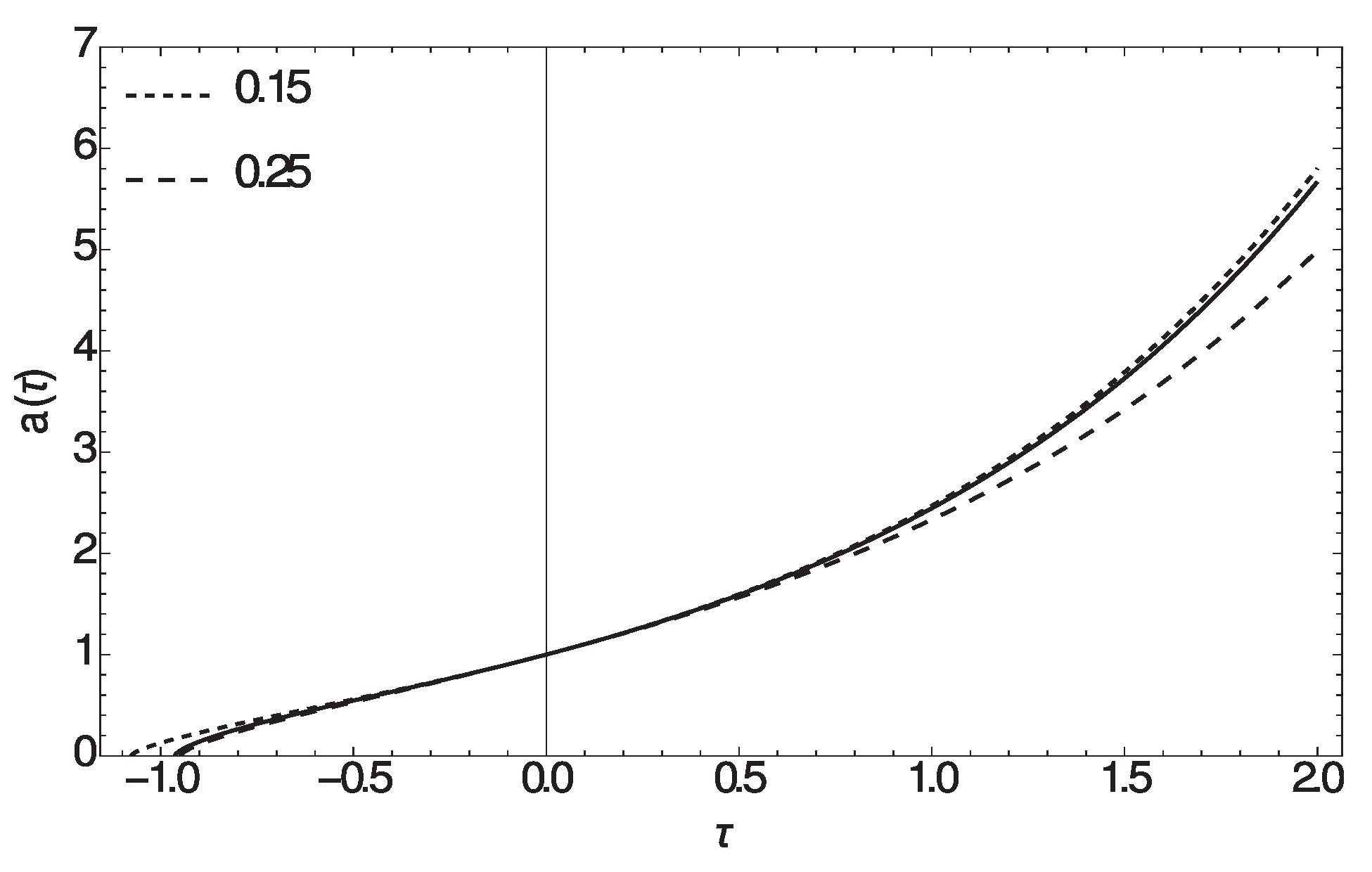
4.1. Evolution of the Scale Factor

In a flat expanding universe, one could see from Equation (32) that the evolution of the dimensionless scale factor is governed by

$$\begin{array}{c}\hfill \frac{da(\tau )}{d\tau }=\frac{1}{2}\left({\Omega }_{0,c_1}{a}^{1+\epsilon }(\tau )+\sqrt{{\Omega }_{0,c_1}^2{a}^{2+2\epsilon }(\tau )+4(\frac{{\Omega }_{0,m}}{a(\tau )}+\frac{{\Omega }_{0,r}}{a^2(\tau )})}\right)\end{array}$$

(34)

in which $\tau \equiv H_{0}t$ is the dimensionless time. This differential equation is solved numerically for two values of ${\Omega }_{0,m}$ and the initial value of $a(0)=1$, and the results are reported in Figure 2. The evolution of the scale factor in the $\Lambda CDM$ model is also shown by a solid line which closely follows a Neumann cosmology with $0.15\lesssim {\Omega }_{0,m}\lesssim 0.25$.

Apart from this numerical solution, one could find the time dependency of the scale factor in some special cases. For example, in early universe, the share of the radiation dominates the right hand side of Equation (34). In this case, the scale factor could be derived as $a(\tau )\propto {\tau }^{1/2}$. Also, in later times, the matter term dominates the rhs of Equation (34) and so we derive $a(\tau )\propto {\tau }^{2/3}$. Finally, at later epochs, the terms corresponding to matter and radiation vanish and ${\Omega }_{c_1}$ start to govern the cosmic evolution. Here, if we have $\epsilon =0$, then the solution to Equation (34) would be exponential, i.e., $a(\tau )\propto \exp ({\Omega }_{0,c_1}\tau )$. These last three statements could be easily derived from Equation (34). On the other hand, in the case of a nonzero $\epsilon$, we need to numerically solve Equation (34) to derive the scale factor.

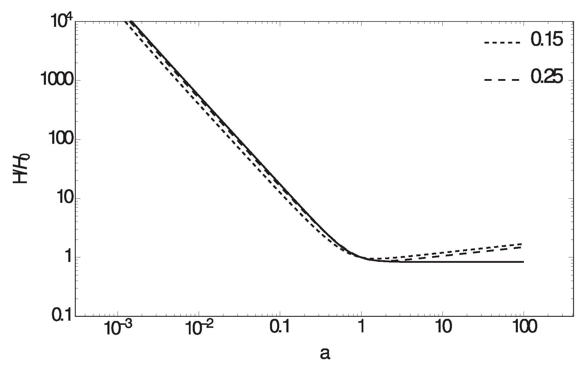
4.2. Hubble and Deceleration Parameter

From Equation (32), one can readily plot the Hubble parameter as a function of the scale factor as you may see in Figure 3. In early cosmic time, the behavior of Hubble parameter in $MOD$ is quite similar to that of the $\Lambda CDM$ model, though the value of Hubble parameter in the former is generally smaller than the latter for $a<1$. However, the behavior of H for $a>1$ is completely dependent to the future evolution of $\zeta$ (or $\epsilon$). The curves in Figure 3 are graphed for $\epsilon =0.15$; however, in the case of $\epsilon =0$, we would have a flat Hubble parameter for $a>1$.

The deceleration parameter q is defined as

$$\begin{array}{ccc}\hfill q=-a\ddot{a}/{\dot{a}}^2& =& -1-\dot{H}/H^2\hfill \end{array}$$

(35)

or equivalently $q=\frac{4\pi G}{H^2(t)}{\sum }_i{\rho }_i(1+3w_i)$. The Friedmann equations have been used to derive this last expression. The evolution of q is graphed in Figure 4 in which one observes $q=1$ in radiation- dominated era, then $q=1/2$ in matter-dominated epoch, and finally $q=-1-\epsilon$ in future cosmic times. Also, to plot q as a function of the normalized scale factor, we have used the next identity:

$$\begin{array}{ccc}\hfill \frac{d}{dt}& =& aH(a)\frac{d}{da}\hfill \end{array}$$

(36)

which converts time derivative of any quantity to its derivative with respect to a. The negativity of the deceleration parameter at present cosmic time is indeed needed to fit observational data to the model as is discussed by Shenavar $and$ Javidan (in preparation). It is also worth noting that, for a model with $\epsilon =0$ (similar to QCD ghost model), one would have a similar behavior except that, in future cosmic time, one derives $q=-1$. This is not plotted in Figure 4.

The negativity of the deceleration parameter in late cosmic time has an important effect on the arguments related to the value of the current cosmic curvature. In fact, using the definition of ${\Omega }_k$, one could derive the time derivative of the curvature density parameter as ${\dot{\Omega }}_k=2{\Omega }_{k}Hq$. Then, if ${\Omega }_k$ has some nonzero value at a very early universe, the late-time negativity of q ensures that the value of ${\Omega }_k$ becomes negligible at present. However, by assuming $c_1=0$, i.e., imposing the Dirichlet boundary condition, the parameter q would always be positive and the ${\Omega }_k$ would not be negligible. This is one of the reasons that one needs cosmological constant $\Lambda$ in the standard model.

4.3. Evolution of the Equation of State Parameter and the Sound Speed

In a flat universe, the total equation of state parameter $w_t$ could be derived from Friedmann equations as follows:

$$\begin{array}{ccc}\hfill w_t& =& -1-\frac{2\dot{H}}{3H^2}.\hfill \end{array}$$

(37)

Now one could simply plot $w_t(a)$ as shown in Figure 5 by using the conversion formula of Equation (36). As this graph shows, the value of $w_t$ is initially very close to $1/3$ because the universe starts from a radiation dominated era. Then, in a matter-dominated era, $w_t$ approaches very rapidly to zero. Finally, at later times, $w_t(a)$ converges (from above) to $w=-1-2\epsilon /3$, which results in an accelerating expansion of the universe. Therefore, in a completely ${\Omega }_{c_1}$-dominated universe, the equation of state must be less than $-1$ for $\epsilon >0$. In this regard, the present model is similar to phantom models of dark energy; however, the existence of a big rip in future, which is the characteristic sign of a phantom scenario, crucially depends on the value of $\epsilon$ at that time. In fact, it is more likely that big rip never happens in Neumann cosmology because all forces of this model are attractive. See the modified Poisson Equation (20) above. In contrast, in a phantom model, the big rip happens when the repulsive force of dark energy rips apart all structures down to subatomic particles [65]. See also Reference [14] for a thorough review. The issue of the behavior of $\epsilon$ and, thus, the possibility of a doomsday scenario in future must be resolved with a more careful study to determine the behavior of $\zeta (t)=1/l(t)$.

See Vagnozzi et al. [66], who compare dynamical dark energy models with $w\ge -1$ and $w<-1$. The authors show that, unlike models which allow values of $w<-1$, a dark energy component with $w\ge -1$ is unable to reduce the tension between observables of high redshift and direct measurements of $H_0$. We will investigate this matter in Shenavar and Javidan (in preparation). It is worthy to note that the curves with smaller ${\Omega }_{0,m}$ tend to $w<-1$ more quickly because the share of ${\Omega }_{0,c_1}$ is larger in these cases. Also, we point out that the parameter $w_t$ of the $\Lambda CDM$ model coincides (approximately) with $0.15\lesssim {\Omega }_{0,m}\lesssim 0.25$ of the present model. See Figure 5.

Another important quantity to be compared with its $\Lambda CDM$ counterpart is the sound speed. For a barotropic fluid, in which the pressure is only dependent to the density $\rho$, the sound speed is defined as $c_s^2=\dot{P}/\dot{\rho }$. This quantity is sometimes called adiabatic sound speed because, in such medium, the entropy per particle is assumed to be constant. As mentioned above, the only physical quantities in $MOD$ model, as in $\Lambda CDM$, are radiation and (baryonic) matter. Thus, the sound speed could be found from Friedmann equations as $c_s^2=({\dot{P}}_r+{\dot{P}}_m)/({\dot{\rho }}_r+{\dot{\rho }}_m)$. Using this equation and changing the time derivatives to derivatives with respect to scale factor Equation (36), one could plot the sound speed as Figure 6. The sound speed squared in a radiation-dominated era is about $1/3$ while, in a matter-dominated era and beyond, tends to zero. The important point here is the positivity of the sound speed of $MOD$ which results in a bounded (non-exponential) rate of the structure formation. Also, from $c_s^2$, one could find the angular size of the sound horizon of $MOD$ and compare it with that of the $\Lambda CDM$ model. This will be done in future.

4.4. Sequence of the Cosmological Epochs

It is easy to check that the present model starts from an unstable radiation-dominated mode, then proceeds toward a matter dominated era, which is also unstable, and then ends its evolution at a stable epoch of ${\Omega }_{c_1}$ domination. See Figure 7. In this plot, we have assumed that ${\Omega }_{0,r}=5\times {10}^{-5}$, ${\Omega }_{0,m}=0.25$, and ${\Omega }_{0,c_1}=1-{\Omega }_{0,m}-{\Omega }_{0,r}$. One could easily check that, by choosing other fractions of ${\Omega }_{0,c_1}$ and ${\Omega }_{0,m}$ and by keeping the radiation density at the order of ${\Omega }_{0,r}\approx {10}^{-5}$, similar behaviors would emerge.

In some alternative cosmologies, the sequence of cosmological epochs is not necessarily as described above. If this happens, one might encounter some problems in dealing with the formation of structures in a matter-dominated era. For example, Amendola et al. [67] have proved that $f(R)$ models of the forms $f(R)=\alpha R^{-n}$ and $f(R)=R+\alpha R^{-n}$ do not show a viable matter-dominated epoch prior to a late-time acceleration for any $n>0$ and $n<-1$. In some cases of $f(R)$ theories, the matter dominated epoch is replaced by an era of cosmic expansion in which the scale factor varies as $a\propto t^{1/2}$, which is cosmologically unacceptable.

Moreover, in the case of scalar-tensor-vector theory of Moffat [52], Jamali and Roshan [68] have shown that there are two radiation-dominated eras, two matter-dominated epochs, and two late time-accelerated phases. In the matter-dominated phases, the growth of the scale factor is found to be as $a(t)\propto t^{0.46}$ and $a(t)\propto t^{0.52}$ slower than the growth in standard model and the present model reported above as $a(t)\propto t^{2/3}$. However, it should be mentioned that, as [69] has reported, the standard MOG possesses a valid sequence of standard cosmological eras.

Because the dimensionless density parameter of the Neumann term is inversely proportional to Hubble parameter, i.e., ${\Omega }_{c_1}\propto 1/H(t)$, it plays no significant role in an early universe which is dominated by radiation and then matter. A similar situation exists in the context of the standard model of cosmology, in which ${\Omega }_{\Lambda }$ is negligible until recent time. However, in the case of $\Lambda CDM$, one deals with the cosmological constant which is very tiny $\Lambda \approx {10}^{-52}$ m${}^{-2}$, while the present model is built on introducing a dimensionless parameter with a value much closer to unity $c_1=0.065$. Also, the density of the cosmological constant, ${\rho }_{\Lambda }=\Lambda c^2/8\pi G$ is always a constant while the density of ${\rho }_{c_1}$ varies with time according to Equation (23).

4.5. Luminosity and Angular Diameter Distances

To compare our model with observational data, we need to measure distances in the universe. Shenavar and Javidan (in preparation) study the behavior of luminosity distance

$$\begin{array}{ccc}\hfill D_L& =& c(1+z){\int }_0^z\frac{d{z}^{\prime }}{H(z^{\prime })}\hfill \end{array}$$

(38)

while the angular diameter distance

$$\begin{array}{ccc}\hfill D_A& =& \frac{c}{1+z}{\int }_0^z\frac{d{z}^{\prime }}{H(z^{\prime })}\hfill \end{array}$$

(39)

is studied by Reference [70]. Both distances are defined for a flat universe. The plot of luminosity distance $D_L$ and angular diameter distance $D_A$ for two values of ${\Omega }_{0,m}$ are shown in Figure 8 and Figure 9, respectively. The analogous curves for $\Lambda CDM$ model too are presented by a solid line in both figures.

As it is shown in the left panel of Figure 8, the luminosity distance of the present model converges to a constant value at $z\gtrsim {10}^4$ while the same curve for the $\Lambda CDM$ model varies linearly. Please note that the left panel is logarithmic on both axes. Fortunately however, to compare the present model with the standard one, it is not needed to observe objects at very high redshifts. The reason is that, as it is shown in the right panel of Figure 8, the luminosity distance in the present model begins to differ significantly from that of the standard model at $z\approx 4$. If the baryonic content of the universe at the present time is larger than a minimal value, say ${\Omega }_{0,m}\gtrsim 0.15$, then the deviation between the two models might be detectable with a precise data analysis at even $z\approx 2.0$. Therefore, it seems that the luminosity distance provides one of the best possibilities to check the viability of the present model. In conclusion, we should say that, although the luminosity distance of the present model is rising with increasing z, it is always smaller than $D_L$ of $\Lambda CDM$ at the same redshift. In fact, $D_L$ of $\Lambda CDM$ acts as an upper boundary of $D_L$ predicted by the present model.

One of the most important consequences of changing the value of $D_L$ is that now the absolute visual magnitude $M_V$ of the objects observed at high redshifts has to be modified (compared to the values derived from standard model). Assuming the apparent visual magnitude as $m_V$, the relation between these two magnitudes is

$$\begin{array}{ccc}\hfill M_V-m_V& =& 5{\log }_{10}(\frac{D_{L,0}}{D_L})\hfill \end{array}$$

in which $D_{L,0}$ is some constant distance, say $10pc$ for near objects or $1Mpc$ in cosmological measurements. Then, one could simply prove that

$$\begin{array}{ccc}\hfill M_{V,MOD}-M_{V,\Lambda CDM}& =& -5{\log }_{10}(\frac{D_L{|}_{MOD}}{D_L{|}_{\Lambda CDM}})\hfill \end{array}$$

(40)

in which $M_{V,MOD}$ is the absolute visual magnitude in our modified model, $M_{V,\Lambda CDM}$ is the absolute visual magnitude in the standard model, $D_L{|}_{MOD}$ is the luminosity distance in the present model, and finally $D_L{|}_{\Lambda CDM}$ is the luminosity distance of the standard model. As it is clear from above equation, the fact that the luminosity distance in the present model is approximately equal to or smaller than that of the standard model leads to the fact that the absolute visual magnitude of the objects would be approximately equal to or larger than the absolute visual magnitude of the standard model. This point must be included especially when one deals with objects at higher redshifts.

In addition, the change in $D_L$ could affect the mass estimations in lensing problem if they lie at relatively high redshifts. In the lensing sample which was used in Reference [28], the lenses lie at redshifts $0.2\le z\le 0.86$, which are relatively low redshifts. Depending to the values of ${\Omega }_{0,m}$ and ${\Omega }_{0,c_1}$, the mass estimation of lenses at higher redshifts might be affected.

The angular diameter distance of the present model too is (almost) always smaller than $D_A$ of $\Lambda CDM$, as shown in Figure 9. The value of $D_A$ for both models decreases when $z\gtrsim 2$, though the decline of $D_A$ in the present model occurs more rapidly. The angular diameter distance provides a good opportunity to confront different cosmological models through the famous “angular size–redshift” problem. See Reference [71] for ane xample. A comparison between $\Lambda CDM$ model and some other cosmologies, including the present one, based on angular size–redshift data is provided by Reference [70].

5. Discussion

5.1. Discussion on the Boundary Condition of GR

Assuming Neumann boundary conditions to solve Equation (11), which results in the solution of Equation (12), is valid as a mathematical possibility. However, this choice of boundary condition would be more motivated if we could enforce it based on some physical backgrounds, i.e., action principle, for example. In fact, the debate on the proper boundary condition of Einstein–Hilbert action dates back to early days of the introduction of general relativity. See Reference [72] for a review on this subject. Especially, one could mention the discussion between de Sitter and Einstein on this matter, which could be considered as the root of relativistic cosmology. In the heart of the debate lies the possibility of a static universe, presumed by Einstein before Hubble’s discovery of the expansion of cosmos [1]. To achieve the relativity of inertia, Einstein proposed a metric of the form $g_{0i}\equiv \infty$ at spatial infinity while other components are zero. However, de Sitter criticized this point of view because it leads to the notion of Newtonian “absolute time” and some invisible masses. In the context of GR, this could be considered as the first mentioning of “dark matter”. In fact, through trying to solve the problem of boundary conditions at spatial infinity, de Sitter and Einstein introduced two distinct cosmic models, the first two models of relativistic cosmology [72].

From a pure mathematical point of view too, the issue of boundary condition seems to be quite controversial in GR. In fact, since Einstein’s field equations contain second-order derivatives of the metric tensor, it could be shown that the Einstein–Hilbert action is not well posed, i.e., the boundary condition of this action is not compatible with the obtained field equations [15]. To cure this problem, however, one could eliminate the surface terms by adding a boundary term to Einstein–Hilbert action. For example, York [73] and Gibbons and Hawking [74] proposed the next action with a surface term

$$\begin{array}{ccc}\hfill S_D& =& \frac{1}{2\kappa }{\int }_{\mathcal{M}}{d}^{D}x\sqrt{-g}R+\frac{1}{\kappa }{\int }_{\partial \mathcal{M}}{d}^{D-1}y\sqrt{|h|}\gamma K\hfill \end{array}$$

(41)

which is invariant under diffeomorphism. In this action, known as YGH action, R is the Ricci scalar, h is the induced metric on the boundary $\partial \mathcal{M}$ with the coordinates $y^i$, K is the extrinsic curvature of the boundary, and g is the determinant of the metric tensor. Also, we have $\gamma =+1$ for time-like and $\gamma =-1$ for space-like boundaries. This action presumes Dirichlet boundary condition by killing all the normal derivatives of the metric tensor on the surface. See Reference [15,45] for a review. It is also worth mentioning that, according to Reference [75], there could be infinitely many boundary terms to make the above action well posed. Therefore, it is not uniquely determined.

On the other hand, by assuming Neumann B.C., Chakraborty [15] and Krishnan and Raju [45] have shown that the action takes the following form:

$$\begin{array}{c}\hfill S_N=\frac{1}{2\kappa }{\int }_{\mathcal{M}}{d}^{D}x\sqrt{-g}R+\frac{D-4}{2\kappa }{\int }_{\partial \mathcal{M}}{d}^{D-1}y\sqrt{|h|}\gamma K\end{array}$$

(42)

with the unique property that the surface term vanishes in $D=4$ dimension. Krishnan and Raju [45] suggest that this property of $S_N$ could be interpreted as follows: “Standard Einstein–Hilbert gravity in four dimensions, without boundary terms, has an interpretation as a Neumann problem”. In addition, Equation (42) is interesting from the point of view of gravitational theories in higher dimensions since it singles out the $D=4$ dimension. In other words, our four dimensional spacetime is not merely one of the possibilities; i.e., $D=4$ is the dimension that one has the elegant Einstein–Hilbert action (without any surface term) if one imposes the Neumann boundary condition. Krishnan and Raju [45] have also shown that, in a three-dimensional space, the Neumann action $S_N$ becomes the Chern–Simons action, which is another interesting feature of this action.

In addition, Maldacena [43] has proved that, by using Neumann B.C., one can derive the semiclassical (or tree level) wavefunction of the universe in 4-D asymptotically de-Sitter or Euclidean anti-de Sitter spacetimes. Since, conformal gravity has many solutions, Neumann B.C. seems to select the Einstein solution out of all possible choices. A more elaborate derivation of the equivalence between Einstein theory and conformal gravity by assuming Neumann B.C. is also provided by Reference [44].

Chakraborty [15] shows that, to impose the Neumann B.C., one has to fix the momentum conjugate on the boundary:

$$\begin{array}{ccc}\hfill {\Pi }^{ij}& =& \sqrt{h}(K^{ij}-K{h}^{ij})\hfill \end{array}$$

(43)

In what follows in this subsection, we will impose the Neumann B.C. on cosmic perturbation equations and then derive the modifications due to this new boundary condition on cosmic equations. To do so, assume a metric of the form

$$d{s}^2=-(1+2\varphi (t,\overrightarrow{x}))d{t}^2+(R^2(t)-2\psi (t,\overrightarrow{x}))d{\overrightarrow{x}}^2.$$

Please note that, unlike metric (Equation (3)), the scale factor $R(t)$ is not included in the potential $\psi$. See Reference [60] for a discussion on the difference between the two metrics. For this metric, the momentum conjugate could be derived as

$$\begin{array}{ccc}\hfill {\Pi }^{ij}& =& -2\dot{R}+2\frac{\dot{R}}{R^2}(R^2\varphi -\psi +\frac{\dot{\psi }}{H})\hfill \end{array}$$

in which the first term on the rhs is of zeroth order while the rest represent the perturbed terms. Neumann boundary condition must be imposed on physical degrees of freedom, i.e., the potentials $\varphi$ and $\psi$. Also, presuming that the time derivative of the 3-curvature perturbation $\psi$ is negligible, i.e., $\dot{\psi }/H\approx 0$, we would have

$$\begin{array}{ccc}\hfill {}^l{\Pi }^{ij}& =& 2\frac{\dot{R}}{R^2}(R^2\varphi -\psi )\hfill \end{array}$$

for the local conjugate momentum. Remembering that $\psi =R^2\Psi$ and assuming ${}^l{\Pi }^{ij}=2\dot{R}{c}_1$ at any time, one would derive $\Phi -\Psi =c_1$ as suggested in Equation (12) (neglecting the anisotropic stress). We note that the Dirichlet B.C. could be reproduced simply by replacing $c_1=0$ in Equation (12).

In deriving the above condition from the Neumann boundary of Equation (43), we assumed the negligibility of the time variation of $\psi$. The validity of this presumption at different scales needs to be studied more carefully and we do not consider it here. Also, another critical assumption is that we only imposed Neumann B.C. on potentials (perturbations) and not the background term, i.e., $-2\dot{R}$, which is related to the geometry of the space. This is justified because we prefer to maintain the underlying geometry intact; otherwise, the whole method of perturbation theory which we used here needs to be revised. In conclusion, the above method provides a possible interpretation for the Neumann boundary condition from an action-principle point of view. The other possible interpretation which was mentioned above and is based on the equivalence between Einstein and conformal gravity would not be discussed here. We should point out that boundary conditions, such as mixed boundary condition, are also possible. See, for instance, Peebles et al. [76] and Peebles [77] impose mixed boundary condition to study the dynamics of the local group.

It is interesting that the possibility of a Neumann B.C. to solve GR field equations has been rarely discussed before. One of the reasons for this shortcoming is that proving the well posedness of GR field equations under a particular boundary condition has been found to be a very difficult task. The well posedness, i.e., the existence and uniqueness of the solution in a small neighborhood, of GR under Cauchy B.C. has been proved by Choquet-Bruhat for the first time and after a long debate. A review on this proof which is based on harmonic coordinates could be found in Reference [19]. Then, Choquet-Bruhat and Geroch [20] proved the theorem of the global existence and uniqueness of GR. See also Reference [78] for a good introduction to this matter. As the authors of Reference [79] have discussed too, the Cauchy problem starts with assuming $(h_{ij},{\Pi }^{ij})$ as a complete set of Cauchy data (initial data). It is not yet clear that, if we change the boundary condition, the proof of “the existence and uniqueness of solutions” would remain intact or not. However, a systematic treatment is needed to prove (or disprove) the well posedness of GR with a Neumann B.C., which is beyond the scopes of the present work.

Another reason for the usual discarding of Neumann B.C. is that the meaning of this boundary condition in a four-dimensional spacetime is not necessarily evident. For example, in the field of numerical relativity, there have been some attempts to impose Neumann B.C. to prevent the violation of constraints [80] or to investigate the numerical stability of Cauchy evolution [81] under the new boundary condition. To impose Neumann B.C., Kidder et al. [80] placed restrictions on the normal derivatives of some characteristic fields while [81] determined ${\partial }_z\Phi$, z being a specific direction in their simulations, at $z=0$. Thus, there had been different conceptions in dealing with Neumann boundary condition. However, now, by the method that References [15,45] present, there is a well-motivated mathematical definition of imposing Neumann B.C. as determining the value of ${\Pi }^{ab}$ on the boundary. Therefore, there is at last a clear definition of “imposing Neumann B.C.” which could guide us through the complexity of GR formalism.

As it is discussed before [28,29,56], assuming Neumann B.C. could lead to three different possibilities. First, by comparing our results with observations, we might realize that the derived value of $c_1$ is very tiny. Of course, in this case, we will conclude that Neumann B.C. is not reliable, i.e., Dirichlet B.C. triumphs. Second, one might derive different values for $c_1$ from various observations, i.e., observations based on lensing, rotation curves of galaxies, CMB, etc. report contradictory results for $c_1$. Then, we would conclude that our fundamental assumption, i.e., Neumann B.C., is not self-consistent and thus excluded. The last possibility is that the value of the Neumann constants $c_1$ which is found from the results of different observations is nonzero and compatible at various scales. In this case, the significance of the Neumann B.C. should not be underestimated.

5.2. Discussion on Mach’s Principle as Boundary Condition

Using the metric in Equation (3), one could derive the field and conservation equations. These are reported in Section 2. Then, one could immediately see from Equation (11) that the scalar fields are not physically independent. Here, one usually concludes that, if the anisotropic stress is negligible, then the two scalars are equal. In other words, it is presumed that ${\partial }_i{\partial }_j(\Phi -\Psi )=0$ leads automatically to $\Phi =\Psi$. However, simple investigation of this partial differential equation ( PDE ) reveals that a presumption is implicitly made about the boundary condition. Namely, it is assumed that $\Phi -\Psi$ vanishes at the boundary, i.e., Dirichlet B.C on the boundary is presumed. On the other hand, by imposing a new boundary condition, e.g., Neumann B.C., the solution to the field equations could substantially change. In conclusion, unless particular boundary conditions are imposed, the gauge conditions do not uniquely fix the potentials. See Reference [82], page 144, for a discussion.

Wheeler [16], too, argues that Einstein field equations, as a system of PDEs, do not suffice to define a solution. These equations must also be supplemented by well-defined boundary conditions which he recognizes as Mach’s principle. Other formulations of Mach’s principle are also possible which might be considered as mathematically vague. See References [16,17,18,21] for more details. According to Wheeler, the role of Mach’s principle, i.e., boundary condition, is to select the solutions of Einstein’s equations based on the physics of the system. This method of selecting solutions is familiar in solving Poisson equations (electrostatics or Newtonian gravitation) which generally goes without a specific name. In fact, as the boundary condition, the Poisson equation is typically supplemented by the statement that the potential decreases as $1/r$. Then, one could see that the distribution of matter (or electric charge) uniquely determines the general form of the potential. If, on the other hand, another boundary condition is imposed, the behaviour of the potential could be entirely different [83]. In the case of general relativity too, the boundary condition is used to select the physically allowable solutions. For example, when one seeks a stellar interior solution, e.g., Tolman–Oppenheimer–Volkoff solution, one might insist that, as the boundary condition, the pressure goes to zero and the solution matches the exterior solution, i.e., the Schwarzschild metric, at the boundary of the star. In the present work, we implement Neumann B.C. on cosmological perturbation equations to pursue a modified model which is more in accord with the observable universe and, thus, free of dark matter and dark energy. As discussed in Section 5.3, by using Neumann B.C., the homogeneity and isotropy of the background universe is still preserved.

However, we do not consider the details here, we only mention that, by imposing Neumann B.C., the super-horizon solutions would also be modified. Moreover, if the parameter $c_1$ is time dependent, then the results could be substantially different from that of References [7,84] depending on the rate of change in $c_1$. In this case, the Weinberg theorem should be modified. See Reference [85] for other models which violate the Weinberg theorem.

5.3. Discussion on the Averaging Procedure

We should note that the averaging procedure defined in Section 3 is carried out on a hypersurface of constant time t. In other words, it is presumed that the averaging integrals are performed instantaneously on the whole of the universe. See Amendola and Tsujikawa [11], page 294, for a discussion on this matter. Of course, one could assume that, in the absence of walls and other huge inhomogeneities, the structures in the cosmos form quite similarly everywhere; thus, the presumption of an instantaneous average is somehow justified. However, as an alternative, the averaging procedure could be done by calculating integrals over the “light-cone” which is a more subtle method. See Reference [86] for a complete description of this procedure. The integration in this method is carried out on a section of spacetime which is “causally” connected with the observer (us). Basically, this type of averaging could lead to quite different consequences (at least for some redshifts and some particular mass distributions) compared to the procedure that we used in Section 3; however, a survey on the difference between the two approaches is beyond the scopes of the present work.

The problem of averaging perturbations at large distances needs to be examined more carefully. In this regard, one might argue that either $(i)$ the perturbed metric, when averaged out on large scales, must result in an isotropic and homogeneous background or $(ii)$ the spacial average of the perturbations needs to vanish on large scales. This latter condition presumes that the perturbed metric provides no contribution to the background metric of the universe at large scale. From an observational point of view, the condition i must always be satisfied. We will call $(i)$ and $(ii)$ the weak and strong smoothness conditions, respectively, and it is the intention of this part to show that a constant $c_1$ satisfies the strong smoothness condition while a time-dependent Neumann parameter $c_1(t)$ is compatible with weak smoothness condition.

To see this, one could readily check that, by using the definition of $\langle A\rangle$ in Section 3, the averaged metric could be found as

$$\begin{array}{c}\hfill \langle d{s}^2\rangle =-d{t}^2+R^2(t)\left(1+2c_1(t)\right){\delta }_{ij}d{x}^{i}d{x}^j\end{array}$$

(44)

in which we have recovered the time dependence of $c_1$ for the sake of completeness of the discussion. The elements of this averaged metric only depend on time while the governing cosmic equations, which are reported in Appendix A, are modified now. Therefore, a time-dependent Neumann parameter changes the form of the Friedmann equations by providing a share into the background equations. However, a suitable rescaling of the scale factor as $R^{\prime }(t)=R(t){\left(1+2c_1(t)\right)}^{1/2}$ shows that the geometry of the metric (44) is equivalent to FLRW geometry at any time. In general, we conclude that a time-dependent Neumann parameter satisfies condition i. Moreover, regarding the pure time dependence of the averaged metric in Equation (44) and the assumption that the anisotropic scalar is negligible, i.e., ${\pi }^S=0$, one concludes that the background universe is essentially a perfect fluid. On the other hand, if $c_1$ is a constant, then the form of the Friedmann equations remains intact as reported in Equation (27). In this case, which is the main focus of this work, the strong smoothness condition is satisfied. Of course, the result in this latter case is again a perfect fluid.

The appearance of the new term, i.e., $c_1(t)$, in the metric only changes large-scale systems. The reason is that we have only changed the boundary condition of the gravitational field. In particular, in the same way that the expansion of the universe does not change the laws governing the nongravitational forces, i.e., electromagnetic, etc., these laws remain intact under appearance of $c_1(t)$ in Equation (44). For example, a typical scattering between subatomic particles happens in a very short time compared to the rate which $R(t)$ or $c_1(t)$ change significantly. Therefore, in calculating a cross section, it is safe to neglect the time evolution of the universe.

6. Conclusions

In this study, we built a model based on the idea that local scale physics might be affected by the global expansion of the universe through a term which is related to the de Sitter scale of acceleration $c{H}_0$. To do so, we used Neumann B.C. instead of the usual Dirichlet B.C to solve Einstein perturbation equations. This new boundary condition is mathematically well motivated, however, its mathematical well posedness is yet to be surveyed.

The outcome of the model is reminiscent of Mach’s principle. The Mach’s principle argues that the condition of the “distant objects of the cosmos” somehow enters into the laws of local mechanics. There are various interpretations and formulations of this principle which are thoroughly presented in Reference [18]. See also References [21] or [87], pages 543–549. However, the present model is based on the idea that “the expansion of the universe” is essential and that the new term enters the equation of motion through presuming Neumann B.C. in this expanding universe (Wheeler’s formulation of Mach’s principle [16]). By imposing a boundary condition, according to Wheeler, one essentially “selects” a specific solution. The Neumann boundary condition which is used here presumes a nonnegligible effect of the distant objects on local dynamics. Another possible path to the present model might be through evaluating the surface term of the generally covariant integral formulation of GR [22] by imposing a Neumann boundary condition.

In the standard model of cosmology, the accelerating expansion of the universe is provided by assuming a constant density of energy due to $\Lambda$. This term provides a repulsive force at large scales in $\Lambda CDM$ while presuming that a dark halo provides a more attractive force (of course through Newtonian force of gravity) at galactic scales. On the other hand, the new term in the present theory, i.e., the term proportional to $c_{1}cH(t)$ in the Poisson equation (Equation (20)), provides more attractive forces at galactic scales while still produces a negative deceleration parameter at later times, i.e., see $q<0$ in Figure 4. Also, the total equation of state parameter $w_t$ tends to $w_t<-1$ at later times, as was shown in Figure 5. The key to understanding this seemingly odd behavior, i.e., making attraction and repulsion at different scales, is that, unlike the $\Lambda CDM$ model with its static $\Lambda$, the new term in our model changes with time because it is proportional to Hubble parameter. As is shown by References [47,48] and here, the existence of a term proportional to $H(t)$ in Friedmann equations could be considered as a model of dark energy.

Unified models of dark matter and dark energy, which rely on “dark fields” instead of dark matter or $\Lambda$ term, have been proposed before. See [11], chapter 8 and references therein, for a brief review on these models. Among these models, one could mention generalized Chaplygin gas model [49], k-essence model [50], and models based on Bose–Einstein condensation [51]. However, these models might encounter problems in dealing with observations at early or late times. For example, the sound speed in a generalized Chaplygin gas model is small at early cosmic times while it shows a growth at later epochs. Compared with the behavior of $c_s^2$ in the $MOD$ model and $\Lambda CDM$ as reported in Figure 6, this evolution of sound speed in generalized Chaplygin gas results in incompatibilities with observations of large-scale structure [11].

However, the observational success of the standard model seems to mostly rely on the fact that $\Lambda CDM$ needs only a few parameters to fit the cosmological observations [9]. Beside the parameters which are usually derived by fitting cosmological data to $\Lambda CDM$ predictions; there are some other parameters presumed at galactic scales. For instance, a NFW profile (introduced by Navarro, Frenk, and White [88]) relies on two free parameters, i.e., the scale length of the halo and its central density. Furthermore, one also needs more parameters to build a successful particle theory of dark matter, e.g., supersymmetry ( SUSY ), which we will not discuss here. In this respect, the present model could be considered quite economical because at galactic scales it relies only on $c_1$. See Equation (20). At cosmic scales too, the Neumann model is dependent to $c_1$, $\epsilon$ and ${\Omega }_{c_1}$, which seems quite parsimonious. Also, it attributes the puzzling phenomena of dark matter and dark energy to the boundary conditions of the field equations (the state of matter distribution at the boundary) or to the presence of new substances or other dark fields.

Admittedly, the question of boundary/initial conditions in cosmology has not been thoroughly studied so far. The same is true about a possible link between local and global dynamics. However, some exceptions could be found in the works of the founders of the standard model. For example, Dicke and Peebles [89] criticize the proposal of Pachner [90,91], who suggested the existence of a connection between local and global dynamics based on Mach’s principle. In fact, Dicke and Peebles argue that the apparent connection proposed by Pachner is only formal, i.e., such effects would be unobservable. In addition, Peebles [1] (part III, pages 361–363) argues that the notion of initial condition is not necessary for a cosmological model unless probably for the fine-tuning problem of very early universe. However, these works do not include a systematic imposition of a new boundary condition and its local effects and they mostly argue, on general grounds, that such modifications would be unnecessary or unobservable.

The degree of reliability of Neumann model needs to be further studied in galactic, cluster, and cosmic scales. At galactic scales, the local and global stability of the systems have to be surveyed. Specifically, by developing the work of Reference [56], one could derive the local stability of a gas + stellar system and compare the results with star formation rate. Moreover, the scaling rules of the $MOD$ model at galactic scales show interesting properties which will be reported in the future. Another challenge is the problem of dwarf galaxies which is well established within the MOND paradigm but seems quite problematic in $\Lambda CDM$ [36].

However, the main issue at cosmic scales remains to be the CMB analysis of MOD. Regarding the analysis which we presented in Section 2, one could see that the $MOD$ model works based on a modified Poisson equation which is indeed of fourth order. See Equation (3) of Reference [56] for the derivation. The homogeneous form of this equation is usually discussed in the theory of linear elasticity and has been named biharmonic equation. The solutions to biharmonic equation include the solutions of Laplace equation. By implementing the solutions of the modified Poisson equation into perturbation equations, one can derive CMB spectrum. This is a delicate issue which would be reported in a following work. However, as the authors of Reference [55] have discussed, there is already a powerful technique to systematically search for a deviation between the two scalar potentials at cosmic scales, i.e., the so-called anisotropic stress function $\eta =\Psi /\Phi$, which hints to possible need for a modification in gravity (at 95% confidence level).

References

1. Peebles, P.J.E. Principles of Physical Cosmology; Princeton University Press: Princeton, NJ, USA, 1994. [Google Scholar]
2. Peebles, P.J.E.; Ratra, B. The Cosmological constant and dark energy. Rev. Mod. Phys. 2003, 75, 559–606. [Google Scholar] [CrossRef] [Green Version]
3. Bardeen, J.M. Gauge Invariant Cosmological Perturbations. Phys. Rev. 1980, D22, 1882–1905. [Google Scholar] [CrossRef]
4. Mukhanov, V.F.; Feldman, H.A.; Brandenberger, R.H. Theory of cosmological perturbations. Part 1. Classical perturbations. Part 2. Quantum theory of perturbations. Part 3. Extensions. Phys. Rept. 1992, 215, 203–333. [Google Scholar] [CrossRef] [Green Version]
5. Bruni, M.; Matarrese, S.; Mollerach, S.; Sonego, S. Perturbations of space-time: Gauge transformations and gauge invariance at second order and beyond. Class. Quant. Grav. 1997, 14, 2585–2606. [Google Scholar] [CrossRef] [Green Version]
6. Malik, K.A.; Wands, D. Cosmological perturbations. Phys. Rep. 2009, 475, 1–51. [Google Scholar] [CrossRef] [Green Version]
7. Weinberg, S. Cosmology; Oxford University Press: Oxford, UK, 2008. [Google Scholar]
8. Sanders, R.H. The Dark Matter Problem; Cambridge University Press: Cambridge, UK, 2010. [Google Scholar]
9. Jain, B.; Khoury, J. Cosmological Tests of Gravity. Ann. Phys. 2010, 325, 1479–1516. [Google Scholar] [CrossRef] [Green Version]
10. Bertone, G.; Tait, T.M.P. A new era in the search for dark matter. Nature 2018, 562, 51–56. [Google Scholar] [CrossRef] [PubMed] [Green Version]
11. Amendola, L.; Tsujikawa, S. Dark Energy; Cambridge University Press: Cambridge, UK, 2015. [Google Scholar]
12. Riess, A.G.; Filippenko, A.V.; Challis, P.; Clocchiatti, A.; Diercks, A.; Garnavich, P.M.; Gillil, R.L.; Hogan, C.J.; Jha, S.; Kirshner, R.P.; et al. Observational evidence from supernovae for an accelerating universe and a cosmological constant. Astron. J. 1998, 116, 1009–1038. [Google Scholar] [CrossRef] [Green Version]
13. Perlmutter, S.; Aldering, G.; Goldhaber, G.; Knop, R.A.; Nugent, P.; Castro, P.G.; Deustua, S.; Fabbro, S.; Goobar, A.; Groom, D.E.; et al. Measurements of Omega and Lambda from 42 high redshift supernovae. Astrophys. J. 1999, 517, 565–586. [Google Scholar] [CrossRef]
14. Bamba, K.; Capozziello, S.; Nojiri, S.; Odintsov, S.D. Dark energy cosmology: The equivalent description via different theoretical models and cosmography tests. Astrophys. Space Sci. 2012, 342, 155–228. [Google Scholar] [CrossRef] [Green Version]
15. Chakraborty, S. Boundary Terms of the Einstein–Hilbert Action. Fundam. Theor. Phys. 2017, 187, 43–59. [Google Scholar] [CrossRef] [Green Version]
16. Wheeler, J.A. Mach’s principle as boundary condition for Einstein’s equations. In Gravitation and Relativity; NASA Goddard Institute for Space Studies: New York, NY, USA, 1966; pp. 303–349. [Google Scholar]
17. Raine, D.J. Mach’s principle and space-time structure. Rep. Prog. Phys. 1981, 44, 1151–1195. [Google Scholar] [CrossRef]
18. Barbour, J.B.; Pfister, H. (Eds.) Mach’s Principle: From Newton’s Bucket to Quantum Gravity; Springer Science & Business Media: Berlin/Heidelberg, Germany, 1995. [Google Scholar]
19. Choquet-Bruhat, Y.; York, J.W., Jr. The Cauchy Problem. In General Relativity and Gravitation. Volume 1—One Hundred Years after the Birth of Albert Einstein; Held, A., Ed.; Plenum Press: New York, NY, USA, 1980; p. 99. [Google Scholar]
20. Choquet-Bruhat, Y.; Geroch, R.P. Global aspects of the Cauchy problem in general relativity. Commun. Math. Phys. 1969, 14, 329–335. [Google Scholar] [CrossRef]
21. Bondi, H.; Samuel, J. The Lense-Thirring effect and Mach’s principle. Phys. Lett. 1997, A228, 121. [Google Scholar] [CrossRef] [Green Version]
22. Sciama, D.W.; Waylen, P.C.; Gilman, R.C. Generally covariant integral formulation of einstein’s field equation. Phys. Rev. 1969, 187, 1762–1766. [Google Scholar] [CrossRef]
23. Thorne, K.S.; Lee, D.L.; Lightman, A.P. Foundations for a Theory of Gravitation Theories. Phys. Rev. D 1973, 7, 3563–3578. [Google Scholar] [CrossRef] [Green Version]
24. Park, I.Y. Boundary dynamics in gravitational theories. arXiv 2018, arXiv:1811.03688. [Google Scholar] [CrossRef] [Green Version]
25. Park, I. Foliation-Based Approach to Quantum Gravity and Applications to Astrophysics. Universe 2019, 5, 71. [Google Scholar] [CrossRef] [Green Version]
26. Park, I.Y. Foliation-based quantization and black hole information. Class. Quant. Grav. 2017, 34, 245005. [Google Scholar] [CrossRef] [Green Version]
27. Witten, E. A Note On Boundary Conditions In Euclidean Gravity. arXiv 2018, arXiv:1805.11559. [Google Scholar]
28. Shenavar, H. Imposing Neumann boundary condition on cosmological perturbation equations and trajectories of particles. Astrophys. Space Sci. 2016, 361, 93. [Google Scholar] [CrossRef]
29. Shenavar, H. Motion of particles in solar and galactic systems by using Neumann boundary condition. Astrophys. Space Sci. 2016, 361, 378. [Google Scholar] [CrossRef]
30. Van Putten, M.H.P.M. Anomalous Galactic Dynamics by Collusion of Rindler and Cosmological Horizons. Astrophys. J. 2017, 837, 22. [Google Scholar] [CrossRef]
31. Van Putten, M.H.P.M. Evidence for galaxy dynamics tracing background cosmology below the de Sitter scale of acceleration. Astrophys. J. 2017, 848, 28. [Google Scholar] [CrossRef] [Green Version]
32. Milgrom, M. A Modification of the Newtonian dynamics as a possible alternative to the hidden mass hypothesis. Astrophys. J. 1983, 270, 365–370. [Google Scholar] [CrossRef]
33. Milgrom, M. A Modification of the Newtonian dynamics: Implications for galaxies. Astrophys. J. 1983, 270, 371–383. [Google Scholar] [CrossRef]
34. Milgrom, M. A modification of the Newtonian dynamics: Implications for galaxy systems. Astrophys. J. 1983, 270, 384–389. [Google Scholar] [CrossRef]
35. Famaey, B.; McGaugh, S. Modified Newtonian Dynamics (MOND): Observational Phenomenology and Relativistic Extensions. Living Rev. Rel. 2012, 15, 10. [Google Scholar] [CrossRef] [Green Version]
36. Kroupa, P. The dark matter crisis: Falsification of the current standard model of cosmology. Publ. Astron. Soc. Austral. 2012, 29, 395–433. [Google Scholar] [CrossRef] [Green Version]
37. Kroupa, P.; Pawlowski, M.; Milgrom, M. The failures of the standard model of cosmology require a new paradigm. Int. J. Mod. Phys. 2012, D21, 1230003. [Google Scholar] [CrossRef] [Green Version]
38. Vagnozzi, S. Recovering a MOND-like acceleration law in mimetic gravity. Class. Quant. Grav. 2017, 34, 185006. [Google Scholar] [CrossRef]
39. Rasanen, S. Dark energy from backreaction. JCAP 2004, 0402, 003. [Google Scholar] [CrossRef] [Green Version]
40. Hirata, C.M.; Seljak, U. Can superhorizon cosmological perturbations explain the acceleration of the Universe? Phys. Rev. D 2005, 72, 083501. [Google Scholar] [CrossRef] [Green Version]
41. Kolb, E.W.; Matarrese, S.; Notari, A.; Riotto, A. The Effect of inhomogeneities on the expansion rate of the universe. Phys. Rev. D 2005, 71, 023524. [Google Scholar] [CrossRef] [Green Version]
42. Martineau, P.; Brandenberger, R.H. The Effects of gravitational back-reaction on cosmological perturbations. Phys. Rev. D 2005, 72, 023507. [Google Scholar] [CrossRef] [Green Version]
43. Maldacena, J. Einstein Gravity from Conformal Gravity. arXiv 2011, arXiv:1105.5632. [Google Scholar]
44. Anastasiou, G.; Olea, R. From conformal to Einstein Gravity. Phys. Rev. D 2016, 94, 086008. [Google Scholar] [CrossRef] [Green Version]
45. Krishnan, C.; Raju, A. A Neumann Boundary Term for Gravity. Mod. Phys. Lett. A 2017, 32, 1750077. [Google Scholar] [CrossRef] [Green Version]
46. Ehlers, J.; Pirani, F.A.; Schild, A. Republication of: The geometry of free fall and light propagation. Gen. Relat. Grav. 2012, 44, 1587–1609. [Google Scholar] [CrossRef]
47. Cai, R.G.; Tuo, Z.L.; Zhang, H.B.; Su, Q. Notes on Ghost Dark Energy. Phys. Rev. D 2011, 84, 123501. [Google Scholar] [CrossRef] [Green Version]
48. Cai, R.G.; Tuo, Z.L.; Wu, Y.B.; Zhao, Y.Y. More on QCD Ghost Dark Energy. Phys. Rev. D 2012, 86, 023511. [Google Scholar] [CrossRef] [Green Version]
49. Bento, M.C.; Bertolami, O.; Sen, A.A. Generalized Chaplygin gas, accelerated expansion and dark energy matter unification. Phys. Rev. D 2002, 66, 043507. [Google Scholar] [CrossRef] [Green Version]
50. Scherrer, R.J. Purely kinetic k-essence as unified dark matter. Phys. Rev. Lett. 2004, 93, 011301. [Google Scholar] [CrossRef] [Green Version]
51. Fukuyama, T.; Morikawa, M.; Tatekawa, T. Cosmic structures via Bose Einstein condensation and its collapse. JCAP 2008, 0806, 033. [Google Scholar] [CrossRef] [Green Version]
52. Moffat, J.W. Scalar-tensor-vector gravity theory. JCAP 2006, 0603, 004. [Google Scholar] [CrossRef]
53. Ellis, G.F.R.; Uzan, J.P. Causal structures in inflation. C. R. Phys. 2015, 16, 928–947. [Google Scholar] [CrossRef]
54. Khoury, J.; Weltman, A. Chameleon cosmology. Phys. Rev. D 2004, 69, 044026. [Google Scholar] [CrossRef]
55. Di Valentino, E.; Melchiorri, A.; Silk, J. Cosmological hints of modified gravity? Phys. Rev. D 2016, 93, 023513. [Google Scholar] [CrossRef] [Green Version]
56. Shenavar, H.; Ghafourian, N. Local stability of galactic discs in modified dynamics. Mon. Not. R. Astron. Soc. 2018, 475, 5603–5617. [Google Scholar] [CrossRef]
57. Pyne, T.; Birkinshaw, M. Beyond the thin lens approximation. Astrophys. J. 1996, 458, 46. [Google Scholar] [CrossRef] [Green Version]
58. Pyne, T.; Carroll, S.M. Higher order gravitational perturbations of the cosmic microwave background. Phys. Rev. D 1996, D53, 2920–2929. [Google Scholar] [CrossRef] [Green Version]
59. Ohanian, H. Gravitation and Spacetime; W. W. Norton: New York, NY, USA, 1976. [Google Scholar]
60. Jacobs, M.W.; Linder, E.V.; Wagoner, R.V. Obtaining the metric of our Universe. Phys. Rev. D 1992, 45, R3292. [Google Scholar] [CrossRef]
61. Zalaletdinov, R.M. Averaging out the Einstein equations and macroscopic space-time geometry. Gen. Relat. Grav. 1992, 24, 1015–1031. [Google Scholar] [CrossRef]
62. Zalaletdinov, R. Towards a theory of macroscopic gravity. Gen. Rel. Grav. 1993, 25, 673–695. [Google Scholar] [CrossRef]
63. Bagheri, S.; Schwarz, D.J. Light propagation in the averaged universe. J. Cosmol. Astropart. Phys. 2014, 1410, 073. [Google Scholar] [CrossRef] [Green Version]
64. Overduin, J.M.; Cooperstock, F.I. Evolution of the scale factor with a variable cosmological term. Phys. Rev. D 1998, 58, 043506. [Google Scholar] [CrossRef] [Green Version]
65. Caldwell, R.R.; Kamionkowski, M.; Weinberg, N.N. Phantom energy and cosmic doomsday. Phys. Rev. Lett. 2003, 91, 071301. [Google Scholar] [CrossRef]
66. Vagnozzi, S.; Dhawan, S.; Gerbino, M.; Freese, K.; Goobar, A.; Mena, O. Constraints on the sum of the neutrino masses in dynamical dark energy models with w(z) ≥ −1 are tighter than those obtained in ΛCDM. Phys. Rev. D 2018, 98, 083501. [Google Scholar] [CrossRef] [Green Version]
67. Amendola, L.; Gannouji, R.; Polarski, D.; Tsujikawa, S. Conditions for the cosmological viability of f(R) dark energy models. Phys. Rev. D 2007, 75, 083504. [Google Scholar] [CrossRef] [Green Version]
68. Jamali, S.; Roshan, M. The phase space analysis of modified gravity (MOG). Eur. Phys. J. C 2016, 76, 490. [Google Scholar] [CrossRef] [Green Version]
69. Jamali, S.; Roshan, M.; Amendola, L. On the cosmology of scalar-tensor-vector gravity theory. J. Cosmol. Astropart. Phys. 2018, 1801, 048. [Google Scholar] [CrossRef] [Green Version]
70. Balakrishna Subramani, V.; Kroupa, P.; Shenavar, H.; Muralidhara, V. Pseudo-evolution of galaxies in Λ CDM cosmology. Mon. Not. R. Astron. Soc. 2019, 488, 3876–3883. [Google Scholar] [CrossRef]
71. Gurvits, L.I.; Kellermann, K.I.; Frey, S. The “angular size—Redshift” relation for compact radio structures in quasars and radio galaxies. Astron. Astrophys. 1999, 342, 378. [Google Scholar]
72. Realdi, M.; Peruzzi, G. Einstein, de Sitter and the beginning of relativistic cosmology in 1917. Gen. Relat. Grav. 2009, 41, 225–247. [Google Scholar] [CrossRef]
73. York, J.W., Jr. Role of conformal three geometry in the dynamics of gravitation. Phys. Rev. Lett. 1972, 28, 1082–1085. [Google Scholar] [CrossRef]
74. Gibbons, G.W.; Hawking, S.W. Action Integrals and Partition Functions in Quantum Gravity. Phys. Rev. D 1977, 15, 2752–2756. [Google Scholar] [CrossRef]
75. Charap, J.M.; Nelson, J.E. Surface Integrals and the Gravitational Action. J. Phys. A 1983, 16, 1661. [Google Scholar] [CrossRef]
76. Peebles, P.J.E.; Tully, R.B.; Shaya, E.J. A Dynamical Model of the Local Group. arXiv 2011, arXiv:1105.5596. [Google Scholar]
77. Peebles, P. Dynamics of the Local Group: The Dwarf Galaxies. arXiv 2017, arXiv:1705.10683. [Google Scholar]
78. Gourgoulhon, E. 3+ 1 Formalism in General Relativity: Bases of Numerical Relativity; Springer Science & Business Media: Berlin/Heidelberg, Germany, 2012; Volume 846. [Google Scholar]
79. Arnowitt, R.L.; Deser, S.; Misner, C.W. The Dynamics of general relativity. Gen. Relat. Grav. 2008, 40, 1997–2027. [Google Scholar] [CrossRef] [Green Version]
80. Kidder, L.E.; Lindblom, L.; Scheel, M.A.; Buchman, L.T.; Pfeiffer, H.P. Boundary conditions for the Einstein evolution system. Phys. Rev. D 2005, 71, 064020. [Google Scholar] [CrossRef] [Green Version]
81. Szilagyi, B.; Gomez, R.; Bishop, N.T.; Winicour, J. Cauchy boundaries in linearized gravitational theory. Phys. Rev. D 2000, 62, 104006. [Google Scholar] [CrossRef] [Green Version]
82. Brill, D.R. Observational contacts of general relativity. In Relativity, Astrophysics and Cosmology, Volume 38: Astrophysics and Space Science Library; Israel, W., Ed.; Springer: Dordrecht, The Netherland, 1973; pp. 127–152. [Google Scholar] [CrossRef]
83. Jackson, J.D. Classical Electrodynamics; Wiley: Hoboken, NJ, USA, 1998. [Google Scholar]
84. Weinberg, S. Adiabatic modes in cosmology. Phys. Rev. D 2003, 67, 123504. [Google Scholar] [CrossRef] [Green Version]
85. Akhshik, M.; Firouzjahi, H.; Jazayeri, S. Cosmological Perturbations and the Weinberg Theorem. J. Cosmol. Astropart. Phys. 2015, 1512, 027. [Google Scholar] [CrossRef] [Green Version]
86. Gasperini, M.; Marozzi, G.; Nugier, F.; Veneziano, G. Light-cone averaging in cosmology: Formalism and applications. J. Cosmol. Astropart. Phys. 2011, 1107, 008. [Google Scholar] [CrossRef] [Green Version]
87. Misner, C.W.; Thorne, K.S.; Wheeler, J.A. Gravitation; W. H. Freeman: San Francisco, CA, USA, 1973. [Google Scholar]
88. Navarro, J.F.; Frenk, C.S.; White, S.D.M. The Structure of cold dark matter halos. Astrophys. J. 1996, 462, 563–575. [Google Scholar] [CrossRef] [Green Version]
89. Dicke, R.H.; Peebles, P.J.E. Evolution of the Solar System and the Expansion of the Universe. Phys. Rev. Lett. 1964, 12, 435. [Google Scholar] [CrossRef]
90. Pachner, J. Mach’s Principle in Classical and Relativistic Physics. Phys. Rev. 1963, 132, 1837–1842. [Google Scholar] [CrossRef]
91. Pachner, J. Problem of Energy in an Expanding Universe. Phys. Rev. B 1965, 137, 1379. [Google Scholar] [CrossRef]
92. Marzke, R.F.; Wheeler, J.A. Gravitation as geometry. I: The geometry of space-time and the geometrodynamical standard meter. In Gravitation and Relativity; WA Benjamin: New York, NY, USA, 1964; pp. 40–64. [Google Scholar]
93. Ehlers, J. Survey of general relativity theory. In Relativity, Astrophysics and Cosmology; Springer: Berlin/Heidelberg, Germany, 1973; pp. 1–125. [Google Scholar]
94. Kundt, W.; Hoffmann, B. Determination of gravitational standard time. In Recent Developments in General Relativity; Pergamon Press: New York, NY, USA, 1962; p. 303. [Google Scholar]
95. Desloge, E.A. A simple variation of the Marzke-Wheeler clock. Gen. Relat. Grav. 1989, 21, 677–681. [Google Scholar] [CrossRef]
96. Trautman, A. Editorial note to: J. Ehlers, F. A. E. Pirani and A. Schild, The geometry of free fall and light propagation. Gen. Relat. Grav. 2012, 44, 1581–1586. [Google Scholar] [CrossRef] [Green Version]
97. Dodelson, S. Modern Cosmology; Academic Press: Amsterdam, The Netherlands, 2003. [Google Scholar]
98. Sofue, Y. Radial distributions of surface mass density and mass-to-luminosity ratio in spiral galaxies. Publ. Astron. Soc. Jpn. 2018, 70, 31. [Google Scholar] [CrossRef]
99. Sofue, Y. Rotation curve decomposition for size-mass relations of bulge, disk, and dark halo components in spiral galaxies. Publ. Astron. Soc. Jpn. 2016, 68, 2. [Google Scholar] [CrossRef] [Green Version]
100. Pilyugin, L.S.; Grebel, E.K.; Zinchenko, I.A.; Kniazev, A.Y. The Abundance Properties of Nearby Late-Type Galaxies. II. the Relation between Abundance Distributions and Surface Brightness Profiles. Astron. J. 2014, 148, 134. [Google Scholar] [CrossRef] [Green Version]
101. Courteau, S. Deep r-Band Photometry for Northern Spiral Galaxies. Astrophys. J. Suppl. Ser. 1996, 103, 363. [Google Scholar] [CrossRef]
102. Courteau, S. Optical Rotation Curves and Linewidths for Tully-Fisher Applications. Astron. J. 1997, 114, 2402. [Google Scholar] [CrossRef]
103. Dirac, P.A.M. The Cosmological constants. Nature 1937, 139, 323. [Google Scholar] [CrossRef]
104. Dirac, P.A.M. New basis for cosmology. Proc. R. Soc. Lond. A 1938, 165, 199–208. [Google Scholar] [CrossRef] [Green Version]
105. Weinberg, S. Gravitation and Cosmology; John Wiley and Sons: New York, NY, USA, 1972. [Google Scholar]
106. Hassani, S. Mathematical Physics: A Modern Introduction to Its Foundations; Springer Science & Business Media: Berlin/Heidelberg, Germany, 2013. [Google Scholar]
107. Schücking, E.L. Cosmology. In Relativity Theory and Astrophysics. Vol.1: Relativity and Cosmology; Ehlers, J., Ed.; American Mathematical Society: Providence, RI, USA, 1967; p. 218. [Google Scholar]
108. Benisty, D.; Guendelman, E.I. Homogeneity of the universe emerging from the Equivalence Principle and Poisson equation: A comparison between Newtonian and MONDian cosmology. arXiv 2019, arXiv:1902.06511. [Google Scholar]
Figure 1. A particle (dashed curve) is falling into the potential well of a massive object (a galaxy) in a homogeneous and isotropic background. The sphere includes all the particles which have already been in causal contact with the central mass under consideration; thus, the radius of the spherical boundary is indeed the size of the particle horizon. The presence of distant objects produces a nontrivial boundary condition Φ Ψ = c 1 on the boundary surface, which we will consider here.
Universe 06 00001 g001
Figure 2. The evolution of scale factor a as a function of dimensionless cosmic time τ H 0 t for Ω 0 , r = 5 × 10 5 , two values of baryonic density namely Ω 0 , m = 0.15 and 0.25 , and Ω 0 , c 1 = 1 Ω 0 , r Ω 0 , m : In addition, we have assumed ε = 0.15 . It could be proved that, by increasing ε , the scale factor in the past epochs remains almost unchanged while the scale factor in future cosmic time increases. The evolution of the scale factor a in the Λ C D M model is also shown by a solid line.
Universe 06 00001 g002
Figure 3. Hubble parameter as a function of scale factor: See Figure 2 for the values of the basic parameters. It could be shown that, by increasing ε , the Hubble parameter in the past epochs remains unchanged while it increases in future cosmic time.
Universe 06 00001 g003
Figure 4. The evolution of the deceleration parameter q as a function of the scale factor: See Figure 2 for the values of the basic parameters. It could be verified that, by increasing ε , the q parameter in the past epochs remains almost unchanged while it decreases in future cosmic time as q = 1 ε .
Universe 06 00001 g004
Figure 5. Evolution of the equation of state w as a function of scale factor a for Ω 0 , r = 5 × 10 5 for two different values of Ω 0 , m : One could prove that, by increasing ε , the equation of state in the past epochs remains almost unchanged while it decreases in future cosmic time as w = 1 2 ε / 3 . The evolution of w in the Λ C D M model is also shown by a solid line.
Universe 06 00001 g005
Figure 6. Evolution of the adiabatic sound speed c s ( a ) 2 as a function of scale factor a: It is straightforward to show that, by changing ε , the adiabatic sound speed remains almost unchanged in all cosmic time.
Universe 06 00001 g006
Figure 7. The evolution of the dimensionless density parameters.
Universe 06 00001 g007
Figure 8. (Left) Luminosity distance D L for Ω 0 , r = 5 × 10 5 and different values of Ω 0 , m in a flat universe: Both vertical and horizontal axes are logarithmic. The luminosity distance in the present model converges to a fixed value at very high redshifts while that of the Λ C D M model continues to grow. (Right) The behavior of D L in relatively small redshifts: One could see that, for most values of Ω 0 , m , the difference between the two models is not negligible even at z 2.0 . One could prove that, by changing ε , the luminosity distance remains almost unchanged in all cosmic time.
Universe 06 00001 g008
Figure 9. The angular diameter distance D A for Ω 0 , r = 5 × 10 5 and different values of Ω 0 , m in a flat universe: It could be verified that, by changing ε , the angular diameter distance slightly changes.
Universe 06 00001 g009