Article

Dynamical Stability of Bulk Viscous Isotropic and Homogeneous Universe

by
Muhammad Sharif
* and
Qanitah Ama-Tul-Mughani
Department of Mathematics, University of the Punjab, Quaid-e-Azam Campus, Lahore-54590, Pakistan
*
Author to whom correspondence should be addressed.
Universe 2019, 5(8), 185; https://doi.org/10.3390/universe5080185
Submission received: 20 July 2019 / Revised: 5 August 2019 / Accepted: 7 August 2019 / Published: 9 August 2019
(This article belongs to the Special Issue Relativistic Astrophysics)

Abstract

:
In this paper, we study the phase space portrait of homogeneous and isotropic universe by taking different coupling functions between dark energy models and bulk viscous dark matter. The dimensionless quantities are introduced to establish an autonomous set of equations. To analyze the stability of the cosmos, we evaluate critical points and respective eigenvalues for different dynamical quantities. For bulk viscous matter and radiation in tachyon coupled field, these points show stable evolution when γ δ but accelerated expansion of the universe for δ > 1 9 . The stability of the universe increases for some stationary points which may correspond to the late-time expansion for the coupled phantom field.
PACS:
04.20.Cv; 95.36.+x; 98.80.-k

1. Introduction

Recent astronomical observations such as type Ia supernova and cosmic microwave background radiations appear to be fairly compatible with the current cosmic accelerated expansion. These observational pieces of evidence have categorized the universe into four basic epochs. In the vacuum energy era, Planck magnitude of the universe transformed to a macroscopic immensity through a rapid expansion named as inflation. Upon reducing the temperature up to 10 3 K, the universe underwent matter-dominated epoch followed by the cosmic radiation state. Ultimately, in the current de Sitter era, the universe is in the phase of accelerating expansion. According to the latest statistics, our cosmos is composed of 95 % dark sectors (dark energy (DE) and dark matter) and 5 % baryonic matter [1,2]. We can observe the baryonic matter with the naked eye while the gravitational effects of other cosmic components confirm their presence.
Dark energy as an anti-gravitational force tends to accelerate the expansion of the cosmos. It has huge negative pressure with very low energy density in contrast to other cosmic components. The hidden characteristics of these dark sectors are still unknown even after the appropriate results of the Λ CDM model. There are two alternative DE model—one is to modify the geometric part of the Einstein–Hilbert action while the other one is to allocate the appropriate form of the energy-momentum tensor like scalar field models [3,4,5,6,7]. Another technique for cosmic evolution can be achieved through the transformation of the barotropic equation of state in Chaplygin gas [8].
Although a Λ CDM model is compatible with current cosmic observations but still no satisfactory argument has been achieved for the coincidence problem. Interaction of DE with dark matter is the novel technique that might address this issue. The interacting DE models have been proposed by several authors [9,10,11,12,13]. It has been found that the interaction between dark matter and DE models can assist to elaborate on the current cosmic evolution. If the DE models have Ω D E Ω D M of the order 1 and an accelerated stable solution, then the coincidence problem can be alleviated. The non-interacting DE models [14,15,16] showed late-time accelerated attractors with Ω D E = 1 , which did not provide an appropriate solution for the coincidence problem. For the coupling, there does not exist any elementary theory that decides a particle form of interaction. It has been shown [17,18] that the coincidence problem can be resolved by selecting the appropriate coupling factors. There are two forms of coupling in the literature named as local and non-local coupling terms. In the local form of interactions, energy density has a direct relation with it [19], whereas non-local forms are directly proportional to Hubble parameter H and energy density. Yang et al. [20] investigated the observational consequences of stable interacting DE models in the light of recent cosmological data.
In the field of cosmology, the autonomous system is another notable technique to study the evolution of the universe. However, this approach does not provide any proper solution but measures the stability of the system efficiently [21]. Phase space analysis also plays a vital role in the inspection of stability for different models by describing momentum as well as a position at each point of the system. Xiao and Zhu [22] investigated dynamical properties of DE models through barotropic fluid in the background of quantum gravity. Shahalam et al. [23] analyzed the stability as well as accelerated behavior of the universe through the interaction of scalar field models with dark matter in the gravitational background of the FRW universe. We have extended their work to study the impact of nonlinear electrodynamics on the stability of FRW universe model through phase space portrait [24]. Recently, Sharif and Mumtaz [25] studied the phase space analysis of locally rotationally symmetric (LRS) Bianchi type I universe by taking different coupling functions between DE models and dark matter. In the present work, we study the effect of bulk viscosity on the stability as well as the expansion of the cosmos by using the dimensionless quantities.
The insertion of the bulk viscosity coefficient in the matter has become a focus of attention due to its remarkable consequences in astrophysics. This is a continuation of the idea of fluid velocity in the surrounding of dissipation and is accepted as a favorable phenomenon in inflation [26,27,28]. It has also been contemplated that bulk viscous fluid as a source of accelerated expansion can account for dark matter as well as late-time expansion of the universe [29]. The cosmological aspects of viscosity can be observed as a measure of the pressure required to reinstate equilibrium position when the expansion of fluids occurs in an expanding universe. Acquaviva and Beesham [30] analyzed the stability of FRW universe dominated by nonlinear bulk viscous matter. Sasidharan and Mathew [31] discussed the asymptotic properties of the FRW universe for three different bulk viscous coefficients and predicted the current cosmic expansion through their solutions. Sharif and Mumtaz [32] studied the effects of viscosity on the expansion of LRS Bianchi type I universe through phase space analysis.
In this paper, we explore stability as well as expanding behavior of FRW universe, by considering the interaction of DE models with bulk viscous dark matter, through phase space analysis. The paper is organized as follows. In Section 2, we provide a basic formalism for dynamical equations and bulk viscous parameter. We establish an autonomous set of equations through the dimensionless variables to analyze the pattern of cosmic evolution. Section 3 contains the phase space portrait of three specific forms of interaction between phantom energy and bulk viscous fluid. The characteristics of tachyon field with Q = γ σ ˙ ϕ is discussed in Section 4. In the final section, we summarize the results.

2. Dynamical Equations

In this section, we compute dynamical equations for bulk viscous matter and DE in the background of isotropic and homogeneous model of universe given by
d s 2 = d t 2 + a 2 ( t ) ( d r 2 + r 2 d θ 2 + r 2 sin 2 θ d ϕ 2 ) ,
such that a ( t ) depicts the scale factor. The viscous energy-momentum tensor [33] has the form
T μ ν = σ u μ u ν + ( p ζ γ C γ ) ( g μ ν + u μ u ν ) ,
where σ , p, ζ and C γ correspond to the energy density, pressure, bulk viscosity and dynamical velocity (canonical momentum) of the fluid, respectively. The dynamical velocity is defined by C γ = ξ u γ and ξ is named as specific enthalpy of a fluid element,
ξ = σ + p ψ ,
with ψ its rest mass density. The dynamical velocity has been contemplated as a generalization of the fluid’s velocity in the presence of dissipation [34]. The bulk viscosity can be measured by γ C γ which is compatible with the idea that it vanishes for an incompressible fluid, i.e., γ C γ = 0 . Moreover, the rest mass density remains conserved along the lines of flow, i.e., γ ( ψ u γ ) = 0 such that ψ = ψ 0 a 3 , where ψ 0 is an integration constant.
Now, we consider the interaction between the phantom field and the dark matter through the coupling Q. This will be helpful to analyze how interaction terms can influence the qualitative behavior of models containing scalar fields and bulk viscous matter. These terms have been studied widely in literature in the context of reheating and inflation [35,36]. The density of the universe remains preserved throughout the evolution, but, for each constituent, it does not hold the conservation law:
σ ˙ m ( 1 3 H ζ a 3 ) + 3 H ( σ m ) ( 1 6 H ζ a 3 ) = Q ,
σ ˙ ϕ ( 1 3 H ζ a 3 ) + 3 H ( σ ϕ + p ϕ ) ( 1 6 H ζ a 3 ) 3 H ζ a 3 p ˙ ϕ = Q ,
σ ˙ t o t + 3 H ( σ t o t + p t o t ) 3 H ζ a 3 [ σ ˙ t o t + p ˙ t o t + 6 H ( σ t o t + p t o t ) ] = 0 ,
where H = a ˙ a , while dot represents the temporal derivative. In addition, p ϕ , p m correspond to pressure and σ ϕ and σ m exhibit the energy density of phantom field and matter (dust), respectively with σ t o t = σ m + σ ϕ and p t o t = p m + p ϕ . In the considered framework, the energy between the components can transform in both ways depending upon the signature of the coupling function. For Q > 0 , the energy outflows from the matter part towards the phantom field and vice versa. In literature, several interaction terms have been studied to observe their effect on the cosmological issues [37,38,39,40].
The field equations, in a spatially flat FRW universe, take the form
H 2 = κ 2 3 ( σ m + σ ϕ ) ,
2 H ˙ + 3 H 2 = κ 2 [ p ϕ + σ ˙ t o t 3 H + ( σ t o t + p ϕ ) ( 1 6 H ζ a 3 ) ] ,
where κ 2 = 8 π G , σ ϕ = 1 2 ϕ 2 ˙ + V ( ϕ ) and p ϕ = 1 2 ϕ 2 ˙ V ( ϕ ) [41]. To transform a set of equations into autonomous system, we introduce the dimensionless quantities as
x = κ ϕ ˙ 6 H , y = κ V 3 H , l = V κ V ,
which satisfy the following relations
d x d U = x ϕ ¨ H ϕ ˙ H ˙ H 2 ,
d y d U = y 3 2 l x + H ˙ H 2 ,
where U = ln a . Through exponential potential, the parameter l becomes a constant value. In this scenario, Equations (4) and (7) can be expressed as
H ˙ H 2 = 3 2 ( x 2 + y 2 1 ) ( 1 3 H ζ a 3 ) ,
ϕ ¨ H ϕ ˙ = 3 + 3 2 l y 2 x + Q H ϕ ˙ 2 1 ( 1 6 H ζ a 3 ) .
The effective equation of state (EoS) and field density parameter [41] are given by
ω e f f = 1 2 H ˙ 3 H 2 ,
Ω D E = κ 2 σ ϕ 3 H 2 = ( x 2 y 2 ) .

3. Coupled Phantom Field
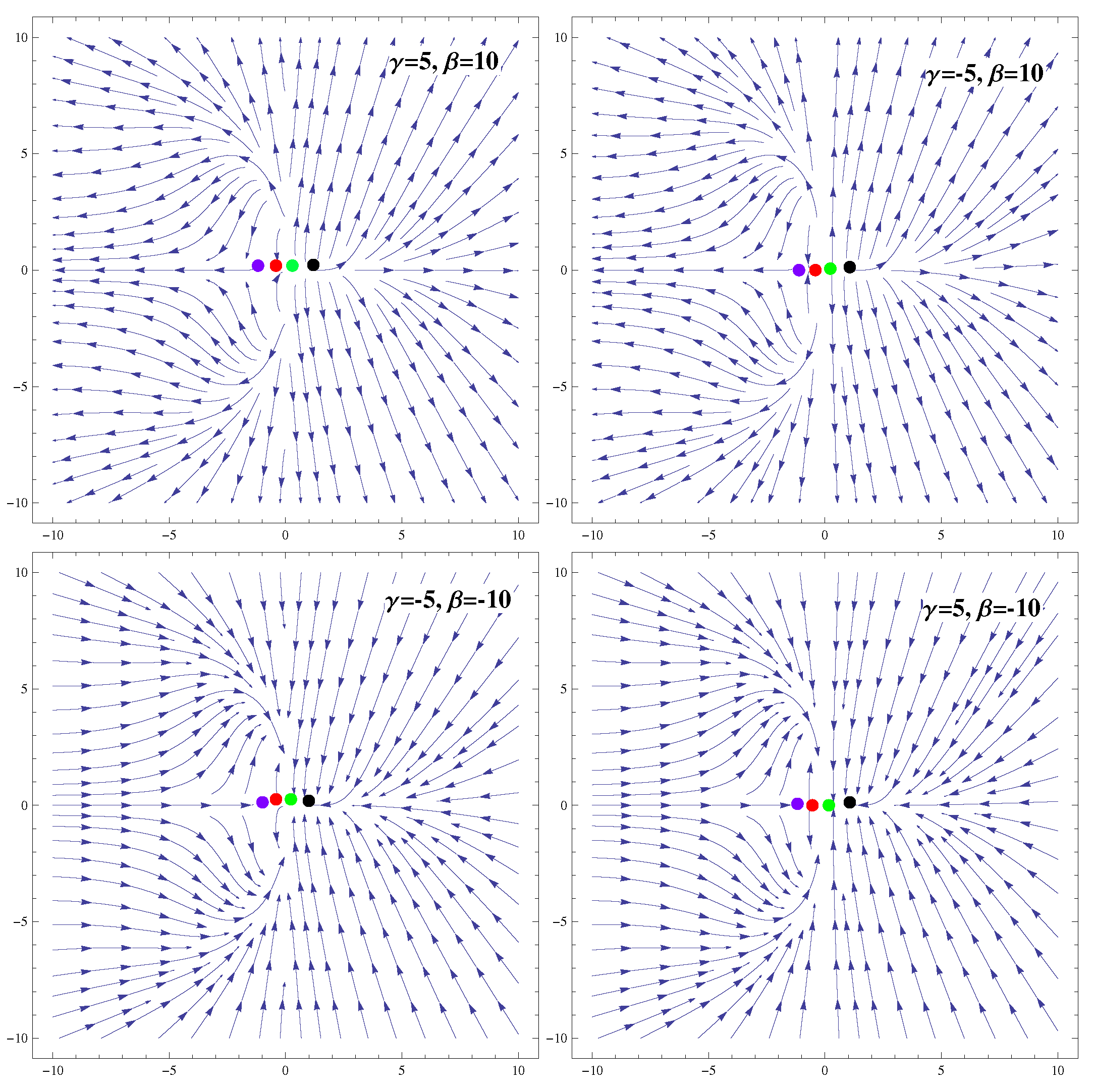
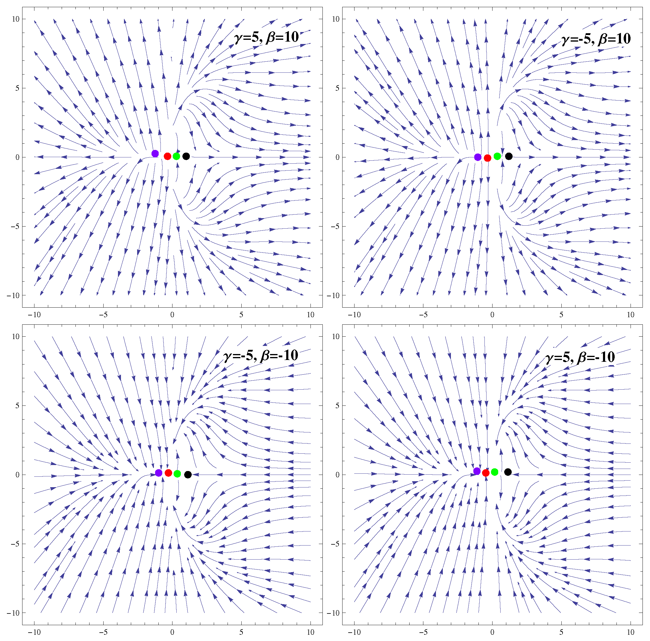
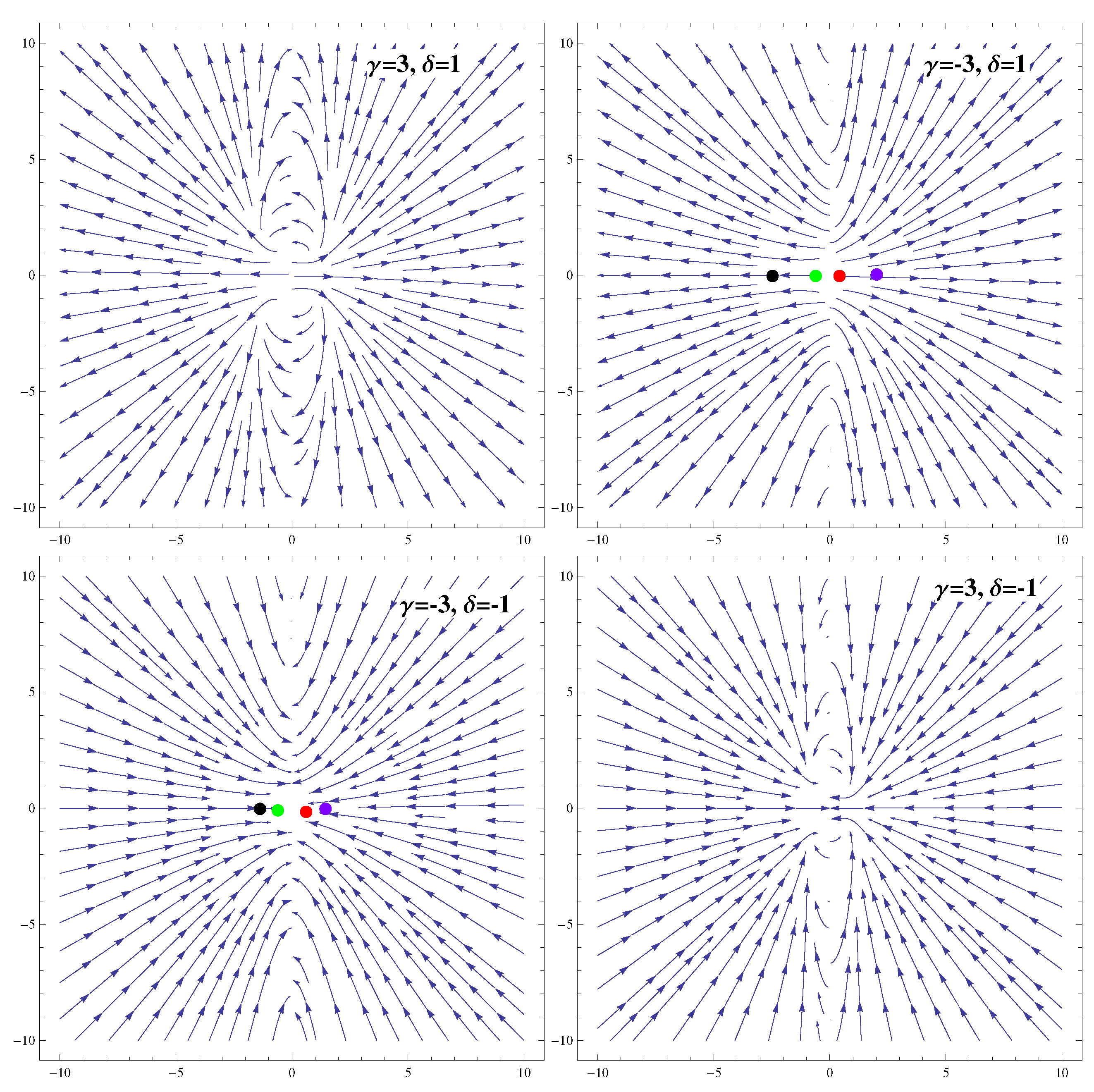
In this section, we examine the impact of different interaction terms (between viscous dark matter and phantom field) on the stability of FRW universe.

3.1. Coupling Q = γ σ ˙ m

We take the coupling function Q = γ σ ˙ m , where γ is an arbitrary constant. For this coupling, Equation (12) leads to
ϕ ¨ H ϕ ˙ = 1 + 3 γ δ ( 1 3 δ γ ) ( 1 6 δ ) γ 1 3 δ γ 3 2 x 2 ( 1 + x 2 + y 2 ) × ( 1 3 δ ) 2 3 3 δ l y 2 2 x 3 ( 1 6 b ) 3 2 l y 2 x 1 1 6 δ 3 ,
where δ = H ζ a 3 is the viscosity factor. The autonomous Equations (9) and (10) reduce to
d x d U = x 1 + 3 γ δ ( 1 3 δ γ ) ( 1 6 δ ) γ 1 3 δ γ 3 2 x 2 ( 1 + x 2 + y 2 ) × ( 1 3 δ ) 2 3 3 δ l y 2 2 x 3 ( 1 6 b ) 3 2 l y 2 x 1 1 6 δ 3 3 x 2 ( x 2 + y 2 1 ) ( 1 3 δ ) ,
d y d U = y 3 2 l x + 3 ( x 2 + y 2 1 ) 2 ( 1 3 δ ) .
To analyze the stability around a critical point, we evaluate its Eigenvalues (EVs) by converting the autonomous set of equations into a Jacobian matrix. Eigenvalues with negative or positive real part correspond to the sink/stable or source/unstable critical nodes, respectively, whereas the EVs with different signatures correspond to the saddle points.
For the stationary node C 1 = ( x , 0 ) , with
x = 1 2 ( 15 γ 2 δ 2 + 162 γ δ 3 + 324 δ 4 2 γ 2 δ 1 15 γ δ 2 108 δ 3 8 γ δ 27 δ 2 + γ + 12 δ + ( 3249 ( δ 2 22 57 δ + 2 57 ) 2 γ 4 + ( 30780 δ 5 30906 δ 4 + 13068 δ 3 2782 δ 2 + 292 δ 12 ) γ 3 + ( 109836 δ 6 119556 δ 5 + 64107 δ 4 20064 δ 3 + 3604 δ 2 340 δ + 13 ) γ 2 + ( 174960 ( δ 3 7 45 δ 2 + 17 135 δ 1 45 ) ( δ 1 6 ) 3 ( 1 3 + δ ) γ + 104976 ( δ 1 6 ) 4 ( 1 3 + δ ) 2 ( δ + 1 3 ) 2 ) 1 2 ) ) 1 2 × ( ( 1 + 6 δ ) ( 1 + 3 δ + γ ) ) 1 ,
the respective EVs are not given due to lengthy expressions. To analyze the impact of γ , δ and l on the stability of stationary points, we portray their dynamical characteristics in Figure 1 and Figure 2 by taking different values of the model parameters. When l > 0 , C 1 shows stable behavior for δ < 0 along with all values of γ as both of its EVs become negative for this range of parameters. This critical point depicts unstable behavior for other possible values of γ and δ as shown in Figure 1. It is mentioned here that the universe experiences accelerated expansion when the relation ( 3 δ + 1 ) x 2 > 1 3 ( 1 + 9 δ ) is satisfied. Figure 2 represents oscillation of the model between unstable and saddle nodes for l < 0 .
For C 2 = ( x , 0 ) with
x = 1 2 ( 15 γ 2 δ 2 + 162 γ δ 3 + 324 δ 4 2 γ 2 δ 1 15 γ δ 2 108 δ 3 8 γ δ 27 δ 2 + γ + 12 δ + ( 3249 ( δ 2 22 57 δ + 2 57 ) 2 γ 4 + ( 30780 δ 5 30906 δ 4 + 13068 δ 3 2782 δ 2 + 292 δ 12 ) γ 3 + ( 109836 δ 6 119556 δ 5 + 64107 δ 4 20064 δ 3 + 3604 δ 2 340 δ + 13 ) γ 2 + ( 174960 ( δ 3 7 45 δ 2 + 17 135 δ 1 45 ) ( δ 1 6 ) 3 ( 1 3 + δ ) γ + 104976 ( δ 1 6 ) 4 ( 1 3 + δ ) 2 ( δ + 1 3 ) 2 ) 1 2 ) ) 1 2 × ( ( 1 + 6 δ ) ( 1 + 3 δ + γ ) ) 1 ,
the EVs correspond to the stable node for negative values of δ and l as all the EVs have negative signature. For positive values of δ and l , this point fluctuates between the unstable and saddle points. When C 3 = ( x , 0 ) with
x = 1 2 ( 15 γ 2 δ 2 + 162 γ δ 3 + 324 δ 4 2 γ 2 δ 1 15 γ δ 2 108 δ 3 8 γ δ 27 δ 2 + γ + 12 δ ( 3249 ( δ 2 22 57 δ + 2 57 ) 2 γ 4 + ( 30780 δ 5 30906 δ 4 + 13068 δ 3 2782 δ 2 + 292 δ 12 ) γ 3 + ( 109836 δ 6 119556 δ 5 + 64107 δ 4 20064 δ 3 + 3604 δ 2 340 δ + 13 ) γ 2 + ( 174960 ( δ 3 7 45 δ 2 + 17 135 δ 1 45 ) ( δ 1 6 ) 3 ( 1 3 + δ ) γ + 104976 ( δ 1 6 ) 4 ( 1 3 + δ ) 2 ( δ + 1 3 ) 2 ) 1 2 ) ) 1 2 × ( ( 1 + 6 δ ) ( 1 + 3 δ + γ ) ) 1 .
It is noted that, for negative values of δ , C 3 depicts stable results for positive as well as negative values of γ . For l < 0 , we get a stable scenario for the positive values of δ .
When C 4 = ( x , 0 ) with
x = 1 2 ( 15 γ 2 δ 2 + 162 γ δ 3 + 324 δ 4 2 γ 2 δ 1 15 γ δ 2 108 δ 3 8 γ δ 27 δ 2 + γ + 12 δ ( 3249 ( δ 2 22 57 δ + 2 57 ) 2 γ 4 + ( 30780 δ 5 30906 δ 4 + 13068 δ 3 2782 δ 2 + 292 δ 12 ) γ 3 + ( 109836 δ 6 119556 δ 5 + 64107 δ 4 20064 δ 3 + 3604 δ 2 340 δ + 13 ) γ 2 + ( 174960 ( δ 3 7 45 δ 2 + 17 135 δ 1 45 ) ( δ 1 6 ) 3 ( 1 3 + δ ) γ + 104976 ( δ 1 6 ) 4 ( 1 3 + δ ) 2 ( δ + 1 3 ) 2 ) 1 2 ) ) 1 2 × ( ( 1 + 6 δ ) ( 1 + 3 δ + γ ) ) 1 ,
the point gives the opposite results to the point C 3 . We achieve more stable results as well as an accelerating era for particular values of parameters as compared to [23]. Most of the stationary points behave as the stable nodes for diverse ranges of parameters as displayed in Figure 1 and Figure 2. It is mentioned that the coincidence problem cannot be resolved through the considered coupling function as density parameter does not attain the proper value, i.e., Ω D E < 0 . The evolutionary results are summarized in Table 1 and acceleration phenomenon is discussed for the parameters γ = ± 20 and δ = ± 1 .

3.2. Coupling Q = γ σ ˙ ϕ

In this scenario, Equation (12) reduces to
ϕ ¨ H ϕ ˙ = 3 + 3 2 l y 2 x + 3 γ 2 x 2 ( 1 3 δ + γ ) ( 1 + x 2 + y 2 ) ( 1 3 δ ) 2 + ( 1 + x 2 y 2 ) ( 1 6 δ ) 1 1 6 δ .
A system of autonomous Equations (9) and (10) takes the form
d x d U = x 3 + 3 2 l y 2 x + 3 γ 2 x 2 ( 1 3 δ + γ ) ( 1 + x 2 + y 2 ) ( 1 3 δ ) 2 + ( 1 + x 2 y 2 ) ( 1 6 δ ) 1 1 6 δ 3 x 2 ( x 2 + y 2 1 ) ( 1 3 δ ) ,
d y d U = y 3 2 l x + 3 ( x 2 + y 2 1 ) 2 ( 1 3 δ ) .
For the stationary node C 1 = ( x , 0 ) with
x = 3 2 ( 1 27 ( 2916 δ 6 + ( 972 γ 972 ) δ 5 + ( 162 γ + 81 γ 2 567 ) δ 4 + 1 2 ( 216 + 486 γ 162 γ 2 ) δ 3 + ( 99 γ 2 180 γ + 18 ) δ 2 + ( 18 γ 2 + 30 γ 12 ) δ + ( γ 1 ) 2 ) 1 2 2 δ 3 + ( γ + 1 3 ) δ 2 + ( 1 3 γ + 2 9 ) δ 1 27 + 1 27 γ ) 1 2 × ( ( δ 1 6 ) ( 3 δ + 1 + γ ) ( δ 1 3 ) ) 1 2 ,
we get stable solutions for positive as well as negative values of γ and δ under some restrictions. For the positive values of dynamical quantities, stable nodes can be achieved with the condition δ γ while, for negative values, the condition is just reversed. It is noted that, for positive values of parameters, we cannot determine the accelerating phase of the universe as the value of effective EoS becomes complex for γ = 20 and δ = 1 . It is observed that this critical point can alleviate the coincidence problem as the density parameter fulfills the criterion, i.e., Ω D E Ω D M = O ( 1 ) for γ < 0 , δ > 0 and γ > 0 , δ < 0 .
When C 2 = ( x , 0 ) with
x = 3 2 ( 1 27 ( 2916 δ 6 + ( 972 γ 972 ) δ 5 + ( 162 γ + 81 γ 2 567 ) δ 4 + 1 2 ( 216 + 486 γ 162 γ 2 ) δ 3 + ( 99 γ 2 180 γ + 18 ) δ 2 + ( 18 γ 2 + 30 γ 12 ) δ + ( γ 1 ) 2 ) 1 2 2 δ 3 + ( γ + 1 3 ) δ 2 + ( 1 3 γ + 2 9 ) δ 1 27 + 1 27 γ ) 1 2 × ( ( δ 1 6 ) ( 3 δ + 1 + γ ) ( δ 1 3 ) ) 1 2 ,
the system fluctuates between the unstable and saddle points for negative values of δ , whereas the stable results can be evaluated for δ > 0 corresponding to all values of l and γ . By increasing the parameter δ , we find more negative EVs depicting stable future attractor. For C 3 = ( x , 0 ) , where
x = 3 2 ( 1 27 ( 2916 δ 6 + ( 972 γ 972 ) δ 5 + ( 162 γ + 81 γ 2 567 ) δ 4 + 1 2 ( 216 + 486 γ 162 γ 2 ) δ 3 + ( 99 γ 2 180 γ + 18 ) δ 2 + ( 18 γ 2 + 30 γ 12 ) δ + ( γ 1 ) 2 ) 1 2 2 δ 3 + ( γ + 1 3 ) δ 2 + ( 1 3 γ + 2 9 ) δ 1 27 + 1 27 γ ) 1 2 × ( ( δ 1 6 ) ( 3 δ + 1 + γ ) ( δ 1 3 ) ) 1 2 .
This fixed point shows unstable or saddle trends except for γ , δ > 0 and l > 0 with γ δ . In this case, the universe undergoes accelerated expansion for negative values of γ . When C 4 = ( x , 0 ) with
x = 3 2 ( 1 27 ( 2916 δ 6 + ( 972 γ 972 ) δ 5 + ( 162 γ + 81 γ 2 567 ) δ 4 + 1 2 ( 216 + 486 γ 162 γ 2 ) δ 3 + ( 99 γ 2 180 γ + 18 ) δ 2 + ( 18 γ 2 + 30 γ 12 ) δ + ( γ 1 ) 2 ) 1 2 2 δ 3 + ( γ + 1 3 ) δ 2 + ( 1 3 γ + 2 9 ) δ 1 27 + 1 27 γ ) 1 2 × ( ( δ 1 6 ) ( 3 δ + 1 + γ ) ( δ 1 3 ) ) 1 2 ,
the system shows varying behavior. When l > 0 , saddle trends can be observed for several combination of the parameters. The results are shown in Figure 3 and Figure 4 and collective behavior in Table 2. The acceleration phenomenon is discussed for the parameters γ = ± 20 and δ = ± 1 . For some choices of model parameters, the critical points become imaginary which can not be displayed on the phase portrait; therefore, their results are summarized in Table 2.

3.3. Coupling Q = γ ( σ ˙ m + σ ˙ ϕ )

Now, we take the coupling as a linear function of σ ˙ m and σ ˙ ϕ which reduces Equation (12) to
ϕ ¨ H ϕ ˙ = 1 + 3 γ δ ( 1 3 δ γ ) ( 1 6 δ ) 3 + 3 γ 2 x 2 ( 1 3 δ + γ ) ( 1 + x 2 + y 2 ) ( 1 3 δ ) 2 + ( 1 + x 2 y 2 ) ( 1 6 δ ) 3 2 l y 2 x 1 1 6 δ + γ ( 1 6 δ ) ( 1 3 δ γ ) 3 2 x 2 ( 1 + x 2 + y 2 ) ( 1 3 δ ) 2 3 3 δ l y 2 2 x 3 ( 1 6 δ ) .
The autonomous system becomes
d x d U = x 1 + 3 γ δ ( 1 3 δ γ ) ( 1 6 δ ) 3 + 3 γ 2 x 2 ( 1 3 δ + γ ) ( 1 + x 2 + y 2 ) ( 1 3 δ ) 2 + ( 1 + x 2 y 2 ) ( 1 6 δ ) 3 2 l y 2 x 1 1 6 δ + γ ( 1 6 δ ) ( 1 3 δ γ ) 3 2 x 2 ( 1 + x 2 + y 2 ) ( 1 3 δ ) 2 3 3 δ l y 2 2 x 3 ( 1 6 δ ) 3 x 2 ( x 2 + y 2 1 ) ( 1 3 δ ) ,
d y d U = y 3 2 l x + 3 ( x 2 + y 2 1 ) 2 ( 1 3 δ ) .
For the critical point C 1 = ( x 1 , 0 ) , the value of x 1 is not given due to lengthy-expression. The corresponding EVs show stable solutions for the positive values of δ and l while the accelerating behavior cannot be determined as the effective EoS gives complex values. However, we obtain the stable as well as saddle zones for l < 0 and δ < 0 corresponding to complete range of γ . For γ < 0 and δ < 0 , we find the accelerated expansion of the universe with oscillating behavior between unstable and saddle nodes. For C 2 = ( x 2 , 0 ) , the critical point varies between the unstable and saddle points for negative values of δ with γ > 0 as well as γ < 0 while the cosmic expansion has been observed in the latter case only. For δ > 0 , the system moves towards more stability corresponding to l > 0 and l < 0 .
When C 3 = ( x 3 , 0 ) , we observe mostly saddle and an unstable trend for the positive vales of l , whereas dynamical stability of C 3 corresponds to l < 0 . We get a stable node for δ , l < 0 and γ > 0 which also lies in the accelerating phase. For C 4 = ( x 4 , 0 ) , the conditions are totally reversed as that of C 3 . Here, we have stable solutions for l > 0 while the negative values of l lead the universe towards instability. The analysis is summarized in Table 3 and the numerical plots are given in Figure 5 and Figure 6.

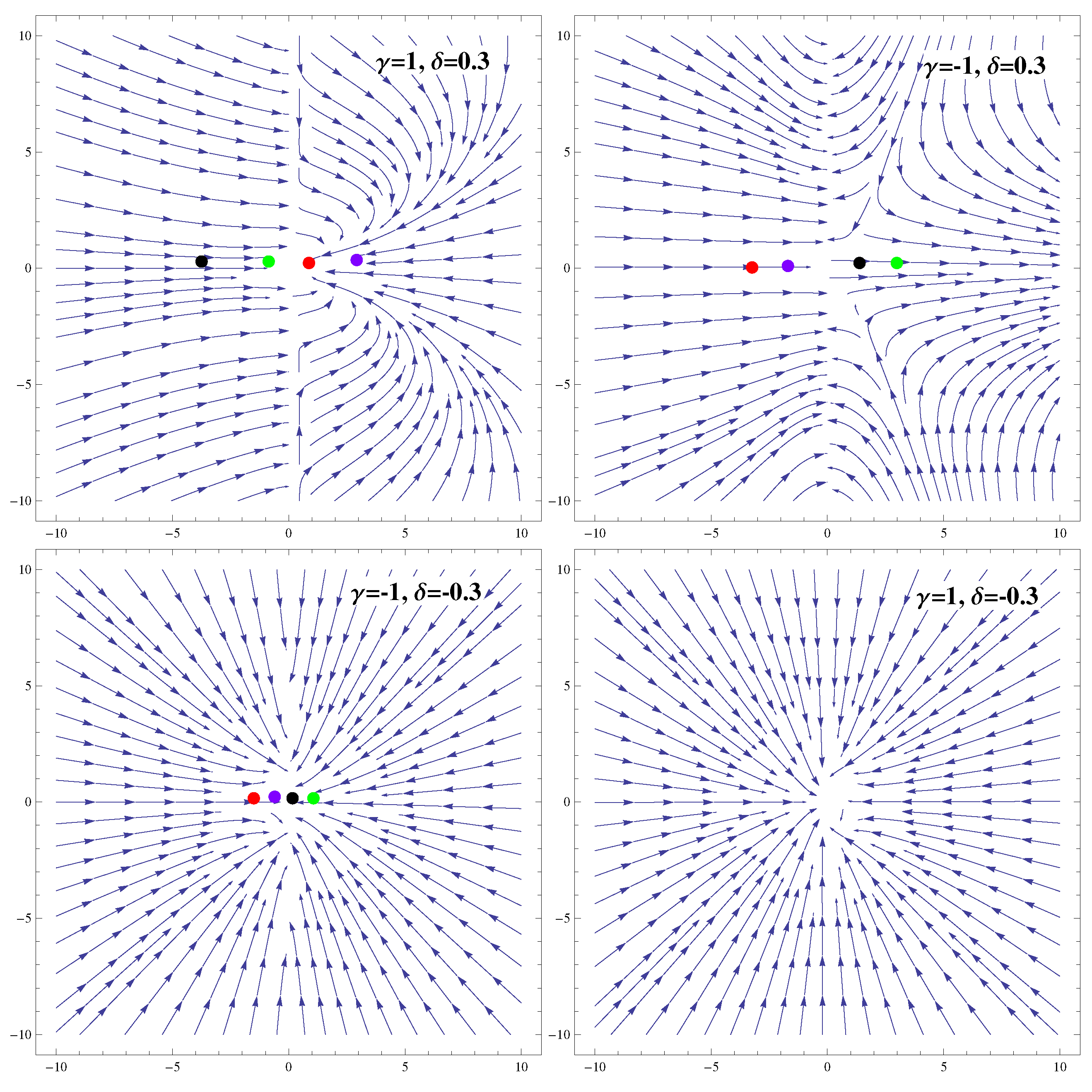
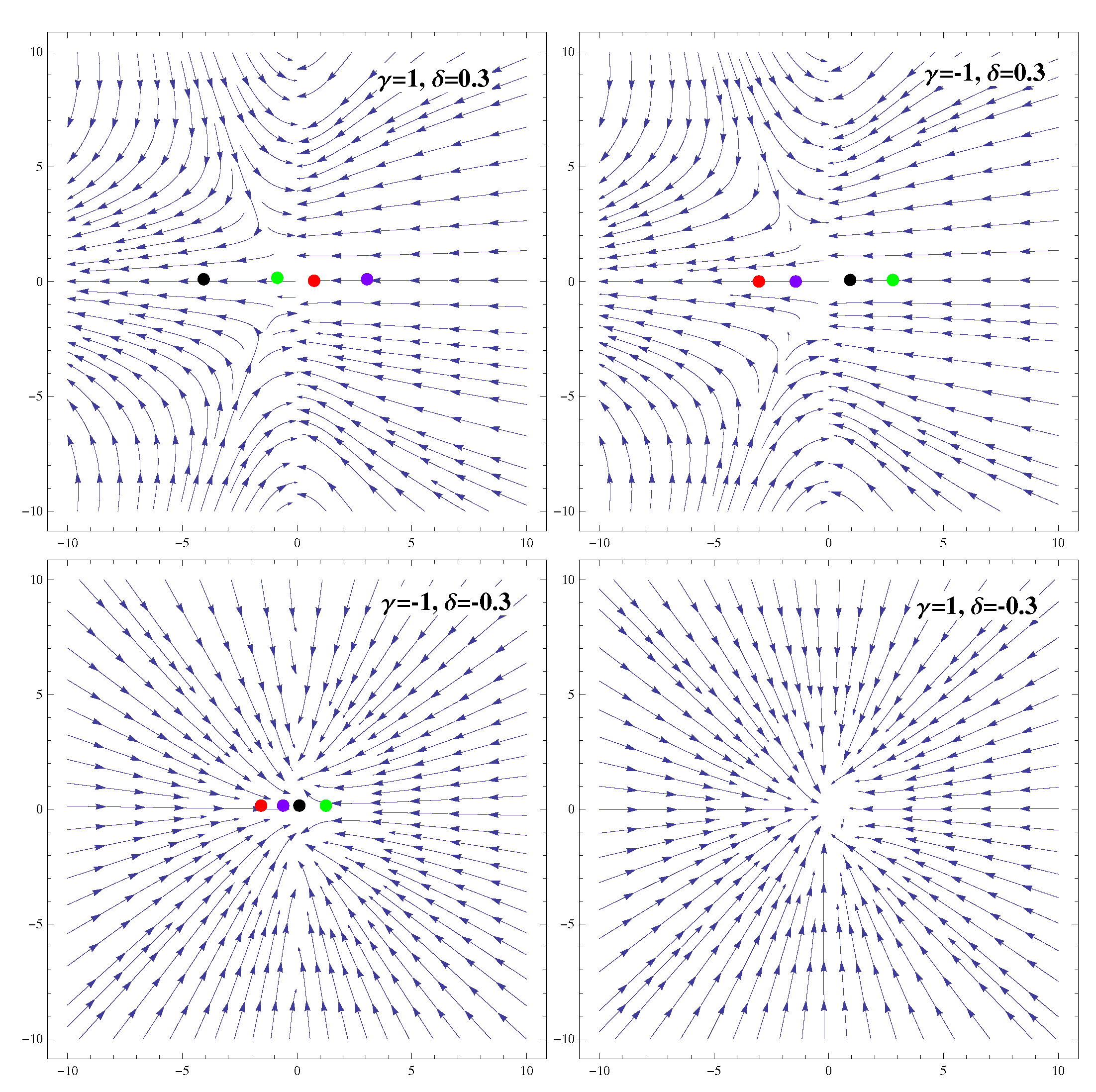
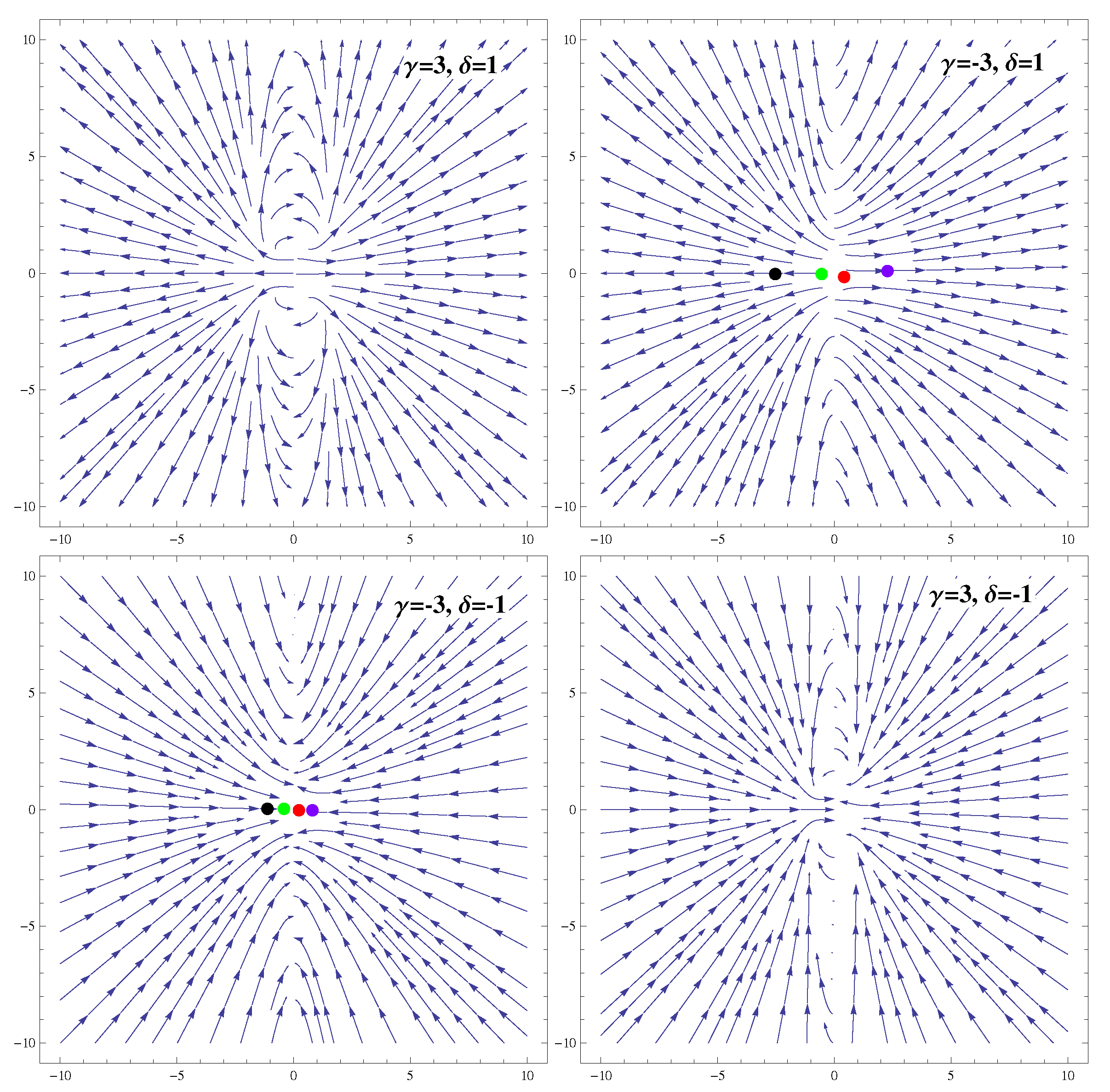
4. Coupled Tachyon Dynamics

In this section, we consider tachyon field as a DE source and interact it with bulk viscous dark matter. In this scenario, the conservation equations turn out to be
σ ˙ m ( 1 3 H ζ a 3 ) + 3 H ( σ m ) ( 1 6 H ζ a 3 ) = Q ,
σ ˙ ϕ ( 1 3 H ζ a 3 ) + 3 H ( σ ϕ + p ϕ ) ( 1 6 H ζ a 3 ) 3 H ζ a 3 p ˙ ϕ = Q ,
where σ ϕ = V ( ϕ ) 1 ϕ ˙ 2 and p ϕ = V ( ϕ ) 1 ϕ ˙ 2 [42]. The evolution equations become
H 2 = κ 2 3 V ( ϕ ) 1 ϕ ˙ 2 + σ m ,
Q 1 ϕ ˙ 2 ϕ ˙ V ( ϕ ) = 3 δ ϕ ˙ 2 V ( ϕ ) V ( ϕ ) + ϕ ¨ ( 2 ϕ ˙ 2 1 ϕ ˙ 2 ) + ϕ ¨ ( 1 ϕ ˙ 2 ) + 3 H ϕ ˙ ( 1 6 δ ) + V ( ϕ ) V ( ϕ ) .
Introducing the dimensionless quantities
x = ϕ ˙ , y = κ V 3 H , l = V κ V V ,
such that the autonomous set of equations turn out to be
d x d U = ϕ ¨ H ϕ ˙ x ,
d y d U = 3 2 l y 2 x y H ˙ H 2 .
For the inverse square potential, the parameter l represents a constant value. We consider the interaction term Q = δ σ ˙ ϕ which reduces Equations (26) and (27) to
H ˙ H 2 = 3 2 ( y 2 1 x 2 1 ) ( 1 3 δ ) ,
ϕ ¨ H ϕ ˙ = 1 + 3 δ + γ ( 1 + 3 δ + γ ) ( 1 + 3 δ ( 2 x 2 ) ) 3 γ δ ( 1 x 2 ) γ 1 3 δ + γ × 3 3 δ y l ( 1 x 2 ) 2 x 3 ( 1 x 2 ) ( 1 6 δ ) + 3 l y ( 1 x 2 ) ( 3 δ x + 1 x ) 3 ( 1 x 2 ) ( 1 6 δ ) .
The effective EoS is given by
ω e f f = 1 2 H ˙ 3 H 2 .
For C 1 = ( 0 , 0 ) , the corresponding EVs are
P 1 = ( 1 4 ) ( 9 ( ( 18 δ 3 + ( 3 γ + 3 ) δ 2 + ( 5 γ + γ 2 + 2 ) δ ( 1 3 ) ( γ 1 ) 2 ) 2 × ( γ 1 + 6 δ ) 2 ) 1 2 + 972 δ 4 1620 δ 3 + ( 378 γ + 783 81 γ 2 ) δ 2 + ( 9 γ 3 + 153 γ 144 ) δ + 9 + 3 γ 2 15 γ + 3 γ 3 ) × ( ( γ + 1 3 δ ) ( γ 1 + 6 δ ) 2 ) 1 ,
P 2 = ( 1 4 ) ( 9 ( ( 18 δ 3 + ( 3 γ + 3 ) δ 2 + ( 5 γ + γ 2 + 2 ) δ ( 1 3 ) ( γ 1 ) 2 ) 2 × ( γ 1 + 6 δ ) 2 ) 1 2 + 972 δ 4 1620 δ 3 + ( 378 γ + 783 81 γ 2 ) δ 2 + ( 9 γ 3 + 153 γ 144 ) δ + 9 + 3 γ 2 15 γ + 3 γ 3 ) × ( ( γ + 1 3 δ ) ( γ 1 + 6 δ ) 2 ) 1 .
It is found that EVs indicate a stable zone only for positive values of γ and δ with the restriction γ δ , while, for the reverse condition, the system moves gradually towards the saddle zone (Figure 7 and Figure 8). Moreover, the effective EoS becomes negative for δ > 1 9 , which corresponds to the accelerated expanding phase of the cosmos, but still the coincidence problem can not be resolved. It is also noticed that this critical point has no dependence on l and shows saddle and unstable trends for other possible values of parameters. When C 2 = ( ± 1 , 0 ) and C 3 = ( ± 1 , ± ( 1 + 3 δ ) 3 l ) , the metric is indeterminant. We cannot evaluate the corresponding EVs as the system becomes undefined at these fixed points for interacting tachyon field model. The results are given in Table 4.

5. Conclusions

In this paper, the impact of bulk viscosity on the stability of FRW universe has been examined through different coupling functions between dark matter and DE models. We have constructed an autonomous set of equations by using dimensionless quantities to inspect the stability of the prescribed system. We have evaluated the stationary nodes by setting x ´ = y ´ = 0 and their respective EVs to explore the effects of γ , δ and l on the stability as well as expansion of the universe.
Firstly, the interaction of dark matter with phantom field has been investigated through EVs for diverse range of parameters (Figure 1, Figure 2, Figure 3, Figure 4, Figure 5 and Figure 6). We analyze the dynamical behavior of three different coupling functions through phase space analysis. For Q = γ σ ˙ m , C 1 and C 2 depict a stable DE model for δ < 0 corresponding to l > 0 and l < 0 , respectively, followed by late accelerated expansion of the cosmos. The critical points C 3 and C 4 correspond to stable points for δ < 0 and δ > 0 , respectively, for all values of γ which completely lie in the DE dominated era as w e f f < 1 3 . For this DE model, all points lie in the de Sitter cosmic phase if the condition ( 3 δ + 1 ) x 2 > 1 3 ( 1 + 9 δ ) is satisfied. For the second coupling Q = γ σ ˙ ϕ , the critical point C 1 shows accelerated stable evolution for γ < 0 , δ > 0 and γ > 0 , δ < 0 which can also alleviate the coincidence problem.
When Q = γ ( σ ˙ m + σ ˙ ϕ ) , we have found stable solutions of C 1 and C 2 for positive values of δ . Finally, for the coupled tachyon field with Q = δ σ ˙ ϕ , the cosmic portrait represents the stable behavior for positive values of γ and δ when γ δ . It is worth mentioning here that these nodes belong to the accelerating phase of the universe if δ > 1 9 . We conclude that the inclusion of a bulk viscosity coefficient in the coupling of dark sectors makes the FRW universe dynamically more stable as compared to [24]. For all the considered couplings, our analysis shows that the coincidence problem can be resolved through the interaction term Q = γ σ ˙ ϕ in the coupled phantom field model in contrast to [23]. In [23], for the coupling Q = γ σ ˙ ϕ , a stable fixed point has been found which behaves as an attractive node but did not depict the accelerating phase of the universe and hence did not solve the coincidence problem. In our work, for the same coupling, the critical point C 1 can alleviate the coincidence problem as it shows the accelerated stable evolution and density parameter fulfills the criterion, i.e., Ω D E Ω D M = O ( 1 ) for γ < 0 , δ > 0 and γ > 0 , δ < 0 .
The coupling Q = γ σ ˙ ϕ alleviates the coincidence problem which shows the compatibility of our results with the current cosmological observations. For future directions, we can adopt this specific form of coupling for other cosmological issues like tension on the determination of H 0 via low-redshift analysis [43] and σ 8 [44], cosmic microwave background anomalies [45] in the light of recent cosmological data.

Author Contributions

M.S. proposed the problem, supervision and finalized the paper while Q.A.-T.-M. did the calculation and prepared the draft.

Funding

This research received no external funding.

Acknowledgments

One of us (Q.A.-T.-M.) would like to thank the Higher Education Commission, Islamabad, Pakistan for its financial support through the Indigenous Ph.D. Fellowship, Phase-II, Batch-III.

Conflicts of Interest

The authors declare no conflict of interest.

References

  1. Sahni, V.; Starobinsky, A.A. The case for a positive cosmological Λ-term. Int. J. Mod. Phys. A 2000, 9, 373. [Google Scholar] [CrossRef]
  2. Tegmark, M.; Strauss, M.A.; Blanton, M.R.; Abazajian, K.; Dodelson, S.; Sandvik, H.; Wang, X.; Weinberg, D.H.; Zehavi, I.; Bahcall, N.A.; et al. Cosmological parameters from SDSS and WMAP. Phys. Rev. D 2004, 69, 03501. [Google Scholar] [CrossRef]
  3. Caldwell, R.R.; Dave, R.; Steinhardt, P.J. Cosmological imprint of an energy component with general equation of state. Phys. Rev. Lett. 1998, 80, 1582. [Google Scholar] [CrossRef]
  4. Chiba, T.; Okabe, T.; Yamaguchi, M. Kinetically driven quintessence. Phys. Rev. D 2000, 62, 023511. [Google Scholar] [CrossRef] [Green Version]
  5. Carroll, S.M.; Hoffman, M.; Trodden, M. Can the dark energy equation-of-state parameter w be less than −1? Phys. Rev. D 2003, 68, 023509. [Google Scholar] [CrossRef]
  6. Chimento, L.P. Extended tachyon field, Chaplygin gas, and solvable k-essence cosmologies. Phys. Rev. D 2004, 69, 123517. [Google Scholar] [CrossRef]
  7. Gorini, V.; Kamenshchik, A.; Moschella, U.; Pasquier, V. Tachyons, scalar fields, and cosmology. Phys. Rev. D 2004, 69, 123512. [Google Scholar] [CrossRef] [Green Version]
  8. Debnath, U.; Banerjee, A.; Chakraborty, S. Role of modified Chaplygin gas in accelerated universe. Class. Quantum Grav. 2004, 21, 5609. [Google Scholar] [CrossRef]
  9. Amendola, L. Coupled quintessence. Phys. Rev. D 2000, 62, 043511. [Google Scholar] [CrossRef] [Green Version]
  10. Zimdahl, W.; Pavon, D.; Chimento, L.P. Interacting quintessence. Phys. Lett. B 2001, 521, 133. [Google Scholar] [CrossRef]
  11. Chimento, L.P. Linear and nonlinear interactions in the dark sector. Phys. Rev. D 2010, 81, 043525. [Google Scholar] [CrossRef]
  12. Verma, M.M.; Pathak, S.D. A Tachyonic scalar field with mutually interacting components. Int. J. Theor. Phys. 2012, 51, 2370. [Google Scholar] [CrossRef]
  13. Verma, M.M.; Pathak, S.D. Shifted cosmological parameter and shifted dust matter in a two-phase tachyonic field universe. Astrophys. Space Sci. 2013, 344, 505. [Google Scholar] [CrossRef]
  14. Wei, H.; Zhang, S.N. Dynamics of quintom and hessence energies in loop quantum cosmology. Phys. Rev. D 2007, 76, 063005. [Google Scholar] [CrossRef] [Green Version]
  15. Setare, M.R.; Saridakis, E.N. Coupled oscillators as models of quintom dark energy. Phys. Lett. B 2008, 668, 177. [Google Scholar] [CrossRef]
  16. Setare, M.R.; Saridakis, E.N. Quintom cosmology with general potentials. Int. J. Mod. Phys. D 2009, 18, 549. [Google Scholar] [CrossRef]
  17. Chimento, L.P.; Jakubi, A.S.; Pavón, D.; Zimdahl, W. Interacting quintessence solution to the coincidence problem. Phys. Rev. D 2003, 67, 083513. [Google Scholar] [CrossRef] [Green Version]
  18. Chimento, L.P.; Pavón, D. Dual interacting cosmologies and late accelerated expansion. Phys. Rev. D 2006, 73, 063511. [Google Scholar] [CrossRef] [Green Version]
  19. Shahalam, M.; Pathak, S.D.; Verma, M.M.; Khlopov, M.Y.; Myrzakulov, R. Dynamics of interacting quintessence. Eur. Phys. J. C 2015, 75, 395. [Google Scholar] [CrossRef]
  20. Yang, W.; Pan, S.; Di Valentino, E.; Nunes, R.C.; Vagnozzie, S.; Motag, D.F. Tale of stable interacting dark energy, observational signatures, and the H0 tension. J. Cosmol. Astropart. Phys. 2018, 2018, 019. [Google Scholar] [CrossRef]
  21. Bogoyavlensky, O.I. Methods in the Qualitative Theory of Dynamical Systems in Astrophysics and Gas Dynamics; Springer: Berlin/Heidelberg, Germany, 1985. [Google Scholar]
  22. Xiao, K.; Zhu, J. Stability analysis of an autonomous system in loop quantum cosmology. Phys. Rev. D 2011, 83, 083501. [Google Scholar] [CrossRef]
  23. Shahalam, M.; Pathak, S.D.; Li, S.; Myrzakulov, R.; Wang, A. Dynamics of coupled phantom and tachyon fields. Eur. Phys. J. C 2017, 77, 686. [Google Scholar] [CrossRef] [Green Version]
  24. Sharif, M.; Mughani, Q.A.T. Stability analysis of coupled phantom and tachyon field models in nonlinear electrodynamics. Int. J. Mod. Phys. D 2019, 28, 1950076. [Google Scholar] [CrossRef]
  25. Sharif, M.; Mumtaz, S. Stability of the universe model coupled with phantom and tachyon fields. Adv. High Energy Phys. 2019, 2019, 6582470. [Google Scholar]
  26. Waga, I.; Falcão, R.C.; Chanda, R. Bulk-viscosity-driven inflationary model. Phys. Rev. D 1986, 33, 1839. [Google Scholar] [CrossRef]
  27. Padmanabhan, T.; Chitre, S.M. Viscous universes. Phys. Lett. A 1987, 120, 433. [Google Scholar] [CrossRef]
  28. Cheng, B. Bulk viscosity in the early universe. Phys. Lett. A 1991, 160, 329. [Google Scholar] [CrossRef]
  29. Zimdahl, W. Bulk viscous cosmology. Phys. Rev. D 1996, 53, 5483. [Google Scholar] [CrossRef]
  30. Acquaviva, G.; Beesham, A. Nonlinear bulk viscosity and the stability of accelerated expansion in FRW spacetime. Phys. Rev. D 2014, 90, 023503. [Google Scholar] [CrossRef] [Green Version]
  31. Sasidharan, A.; Mathew, T.K. Phase space analysis of bulk viscous matter dominated universe. J. High Energy Phys. 2016, 2016, 138. [Google Scholar] [CrossRef]
  32. Sharif, M.; Mumtaz, S. Stability analysis of bulk viscous anisotropic universe model. Astrophys. Space Sci. 2017, 362, 205. [Google Scholar] [CrossRef]
  33. Disconzi, M.M. On the well-posedness of relativistic viscous fluids. Nonlinearity 2014, 27, 1915. [Google Scholar] [CrossRef]
  34. Disconzi, M.M.; Kephart, T.W.; Scherrer, R.J. New approach to cosmological bulk viscosity. Phys. Rev. D 2015, 91, 043532. [Google Scholar] [CrossRef] [Green Version]
  35. Albrecht, A.; Steinhardt, P.J.; Turner, M.S.; Wilczek, F. Reheating an inflationary universe. Phys. Rev. Lett. 1982, 48, 1437. [Google Scholar] [CrossRef]
  36. Berera, A. Warm inflation. Phys. Rev. Lett. 1995, 75, 3218. [Google Scholar] [CrossRef]
  37. Wang, B.; Gong, Y.; Abdalla, E. Transition of the dark energy equation of state in an interacting holographic dark energy model. Phys. Lett. B 2005, 624, 141. [Google Scholar] [CrossRef]
  38. Gumjudpai, B.; Naskar, T.; Sami, M.; Tsujikawa, S. Coupled dark energy: Towards a general description of the dynamics. J. Cosmol. Astropart. Phys. 2005, 2005, 0506. [Google Scholar] [CrossRef]
  39. Campo, S.D.; Herrera, R.; Pavon, D. H(z) Diagnostics on the nature of dark eneryg. Int. J. Mod. Phys. D 2011, 20, 561. [Google Scholar] [CrossRef]
  40. Wei, H.; Cai, R.G. K-chameleon and the coincidence problem. Phys. Rev. D 2005, 71, 043504. [Google Scholar] [CrossRef] [Green Version]
  41. Caldwell, R.R. A phantom menace? Cosmological consequences of a dark energy component with super-negative equation of state. Phys. Lett. B 2002, 545, 23. [Google Scholar] [CrossRef]
  42. Sen, A. Rolling tachyon. J. High Energy Phys. 2002, 2002, 048. [Google Scholar] [CrossRef]
  43. Marra, V.; Amendola, L.; Sawicki, I.; Valkenburg, W. Cosmic variance and the measurement of the local Hubble parameter. Phys. Rev. Lett. 2013, 110, 241305. [Google Scholar] [CrossRef]
  44. Battye, R.A.; Charnock, T.; Moss, A. Tension between the power spectrum of density perturbations measured on large and small scales. Phys. Rev. D 2015, 91, 103508. [Google Scholar] [CrossRef]
  45. Schwarz, D.J.; Copi, C.J.; Huterer, D.; Starkman, G.D. CMB Anomalies after Planck. Class. Quant. Grav. 2016, 33, 184001. [Google Scholar] [CrossRef]
Figure 1. Phase plane portrait of phantom universe for Q = δ σ ˙ m and l > 0 with C 1 (black), C 2 (purple), C 3 (green), C 4 (red).
Universe 05 00185 g001
Figure 2. Phase plane portrait of phantom universe for Q = δ σ ˙ m with l < 0 .
Universe 05 00185 g002
Figure 3. Phase plane portrait of phantom universe for Q = γ σ ˙ ϕ with l > 0 .
Universe 05 00185 g003
Figure 4. Phase plane portrait of phantom universe for Q = γ σ ˙ ϕ with l < 0 .
Universe 05 00185 g004
Figure 5. Phase plane portrait of phantom universe for Q = γ ( σ ˙ m + σ ˙ ϕ ) with l > 0 .
Universe 05 00185 g005
Figure 6. Phase plane portrait of phantom universe for Q = γ ( σ ˙ m + σ ˙ ϕ ) with l < 0 .
Universe 05 00185 g006
Figure 7. Phase plane portrait of tachyon universe for Q = δ σ ˙ ϕ with l > 0 .
Universe 05 00185 g007
Figure 8. Phase plane portrait of tachyon universe for Q = δ σ ˙ ϕ with l < 0 .
Universe 05 00185 g008
Table 1. Stability analysis of phantom universe for Q = γ σ ˙ m .
Ranges of Model ParametersStabilityAcceleration
For ( l > 0 ) , C 1
γ < 0 , δ > 0 unstableYes
γ < 0 , δ < 0 stableYes
γ > 0 , δ < 0 stableYes
γ > 0 , δ > 0 unstableYes
C 2
γ < 0 , δ > 0 saddleYes
γ < 0 , δ < 0 saddleYes
γ > 0 , δ < 0 saddleYes
γ > 0 , δ > 0 unstableYes
C 3
γ < 0 , δ > 0 unstableYes
γ < 0 , δ < 0 stableNo
γ > 0 , δ < 0 stableNo
γ > 0 , δ > 0 unstableYes
C 4
γ < 0 , δ > 0 stableYes
γ < 0 , δ < 0 unstableNo
γ > 0 , δ < 0 unstableNo
γ > 0 , δ > 0 stableYes
For ( l < 0 ) , C 1
γ < 0 , δ > 0 unstableYes
γ < 0 , δ < 0 saddleYes
γ > 0 , δ < 0 saddleYes
γ > 0 , δ > 0 unstableYes
C 2
γ < 0 , δ > 0 unstableYes
γ < 0 , δ < 0 stableYes
γ > 0 , δ < 0 stableYes
γ > 0 , δ > 0 unstableYes
C 3
γ < 0 , δ > 0 stableYes
γ < 0 , δ < 0 unstableNo
γ > 0 , δ < 0 unstableNo
γ > 0 , δ > 0 stableYes
C 4
γ < 0 , δ > 0 unstableYes
γ < 0 , δ < 0 stableNo
γ > 0 , δ < 0 stableNo
γ > 0 , δ > 0 unstableYes
Table 2. Stability analysis of phantom universe for Q = γ σ ˙ ϕ .
Ranges of Model ParametersStabilityAcceleration
For ( l > 0 ) , C 1
γ < 0 , δ > 0 stableYes
γ < 0 , δ < 0 stable if | δ | γ No
γ > 0 , δ < 0 stable if | δ | γ Yes
γ > 0 , δ > 0 stable for δ γ -
C 2
γ < 0 , δ > 0 stableYes
γ < 0 , δ < 0 unstable for δ γ No
saddle for γ δ
γ > 0 , δ < 0 saddleYes
γ > 0 , δ > 0 stable-
C 3
γ < 0 , δ > 0 saddleYes
γ < 0 , δ < 0 saddleYes
γ > 0 , δ < 0 unstableNo
γ > 0 , δ > 0 stable for γ δ ,-
C 4
γ < 0 , δ > 0 saddleYes
γ < 0 , δ < 0 saddleYes
γ > 0 , δ < 0 unstableNo
γ > 0 , δ > 0 stable for γ δ ,-
For ( l < 0 ) , C 1
γ < 0 , δ > 0 stableYes
γ < 0 , δ < 0 unstable for δ γ No
saddle for γ δ
γ > 0 , δ < 0 saddleYes
γ > 0 , δ > 0 stable for δ γ ,-
saddle for γ δ
C 2
γ < 0 , δ > 0 stableYes
γ < 0 , δ < 0 stable for γ δ ,No
γ > 0 , δ < 0 stableYes
γ > 0 , δ > 0 stable-
C 3
γ < 0 , δ > 0 saddleYes
γ < 0 , δ < 0 stable for δ γ ,Yes
unstable for γ δ
γ > 0 , δ < 0 unstableNo
γ > 0 , δ > 0 stable for γ δ -
C 4
γ < 0 , δ > 0 saddleYes
γ < 0 , δ < 0 saddleYes
γ > 0 , δ < 0 unstableNo
γ > 0 , δ > 0 stable for γ δ ,-
Table 3. Stability analysis of the phantom universe for Q = γ ( σ ˙ m + σ ˙ ϕ ) .
Ranges of Model ParametersStabilityAcceleration
For ( l > 0 ) , C 1
γ < 0 , δ > 0 stable-
γ < 0 , δ < 0 stable for δ γ ,Yes
γ > 0 , δ < 0 saddle/unstableNo
γ > 0 , δ > 0 stable-
C 2
γ < 0 , δ > 0 stable-
γ < 0 , δ < 0 saddle/unstableYes
γ > 0 , δ < 0 saddle/unstableNo
γ > 0 , δ > 0 stable-
C 3
γ < 0 , δ > 0 unstable-
γ < 0 , δ < 0 saddle/unstableNo
γ > 0 , δ < 0 saddleYes
γ > 0 , δ > 0 stable for δ γ ,-
C 4
γ < 0 , δ > 0 saddle-
γ < 0 , δ < 0 stableNo
γ > 0 , δ < 0 stableYes
γ > 0 , δ > 0 stable for γ δ -
For ( l < 0 ) , C 1
γ < 0 , δ > 0 stable-
γ < 0 , δ < 0 stable/saddleYes
γ > 0 , δ < 0 saddleNo
γ > 0 , δ > 0 stable-
C 2
γ < 0 , δ > 0 stable-
γ < 0 , δ < 0 stableYes
γ > 0 , δ < 0 saddle/unstableNo
γ > 0 , δ > 0 stable-
C 3
γ < 0 , δ > 0 saddle-
γ < 0 , δ < 0 stable for δ γ ,No
γ > 0 , δ < 0 stableYes
γ > 0 , δ > 0 stable for δ γ ,-
C 4
γ < 0 , δ > 0 unstable-
γ < 0 , δ < 0 saddle/unstableNo
γ > 0 , δ < 0 saddleYes
γ > 0 , δ > 0 stable/saddle-
Table 4. Stability analysis of tachyon universe for Q = δ σ ˙ ϕ .
Ranges of Model ParametersStabilityAcceleration
C 1
γ < 0 , δ > 0 saddleYes for δ > 1 9
γ < 0 , δ < 0 saddle/unstable forNo
γ > 0 , δ < 0 unstableNo
γ > 0 , δ > 0 saddle for δ γ ,Yes for δ > 1 9
stable for γ δ

