A HERO for General Relativity


Ministero dell’Istruzione, dell’Università e della Ricerca (M.I.U.R.)-Istruzione, Viale Unità di Italia 68, 70125 Bari (BA), Italy
Universe 2019, 5(7), 165; https://doi.org/10.3390/universe5070165
Submission received: 14 June 2019
/
Revised: 29 June 2019
/
Accepted: 1 July 2019
/
Published: 5 July 2019
(This article belongs to the Special Issue Rotation Effects in Relativity)
Abstract
HERO (Highly Eccentric Relativity Orbiter) is a space-based mission concept aimed to perform several tests of post-Newtonian gravity around the Earth with a preferably drag-free spacecraft moving along a highly elliptical path fixed in its plane undergoing a relatively fast secular precession. We considered two possible scenarios—a fast, 4-h orbit with high perigee height of and a slow, 21-h path with a low perigee height of . HERO may detect, for the first time, the post-Newtonian orbital effects induced by the mass quadrupole moment of the Earth which, among other things, affects the semimajor axis a via a secular trend of ≃4–12 , depending on the orbital configuration. Recently, the secular decay of the semimajor axis of the passive satellite LARES was measured with an error as little as . Also the post-Newtonian spin dipole (Lense-Thirring) and mass monopole (Schwarzschild) effects could be tested to a high accuracy depending on the level of compensation of the non-gravitational perturbations, not treated here. Moreover, the large eccentricity of the orbit would allow one to constrain several long-range modified models of gravity and accurately measure the gravitational red-shift as well. Each of the six Keplerian orbital elements could be individually monitored to extract the signature, or they could be suitably combined in order to disentangle the post-Newtonian effect(s) of interest from the competing mismodeled Newtonian secular precessions induced by the zonal harmonic multipoles of the geopotential. In the latter case, the systematic uncertainty due to the current formal errors of a recent global Earth’s gravity field model are better than for all the post-Newtonian effects considered, with a peak of for the Schwarzschild-like shifts. Instead, the gravitomagnetic spin octupole precessions are too small to be detectable.
1. Introduction
The (slow) motion of a test particle moving in spacetime (weakly) deformed by the mass-energy content of an isolated, axially symmetric rotating body of mass M, angular momentum , polar and equatorial radii , ellipticity , dimensionless quadrupole mass moment exhibits several post-Newtonian (pN) features. Some of them have never been put to the test so far because of their smallness; they are the gravitoelectric and gravitomagnetic effects associated with the asphericity of the central body induced by its mass quadrupole and spin octupole moments, respectively [1,2,3,4,5,6].
Instead, the pN orbital effects which have been extensively tested so far in several terrestrial and astronomical scenarios are the gravitoelectric and gravitomagnetic precessions due to the mass monopole and spin dipole moments, respectively. The former is responsible for the time-honored, previously anomalous perihelion precession of Mercury [7], whose explanation by Reference [8] was the first empirical success of his newly born theory of gravitation. It was later repeatedly measured with radar measurements of Mercury itself [9,10], of other inner planets [11,12], and of the asteroid Icarus [13,14] as well. Binary pulsars [15] and Earth’s artificial satellites [16,17] have also been used. The latter is the so-called Lense-Thirring effect [18,19,20,21,22], which is currently under scrutiny in the Earth’s surrounding with the geodetic satellites of the LAGEOS family; see, for example, Renzetti [23], and Lucchesi et al. [24], and references therein. Another gravitomagnetic effect—the Pugh-Schiff rates of change of orbiting gyroscopes [25,26]—was successfully tested in the field of the Earth with the dedicated Gravity Probe B (GP-B) spaceborne mission a few years ago [27,28] to a accuracy level, despite the originally expected error level of the order of [29].
By assuming the validity of general relativity, its mass quadrupole and spin octupole accelerations are, to the first post-Newtonian (pN) order,
where G is the Newtonian constant of gravitation, is the gravitational parameter of the primary, c is the speed of light in vacuum, is the unit vector of the rotational axis,
is the cosine of the angle between the directions of the body’s angular momentum and the orbiter’s position vector , and
are the components of the particle’s velocity along the radial direction and the primary’s spin respectively. The averaged rates of change of the semimajor axis a, the eccentricity e, the inclination I, the longitude of the ascending node and the argument of pericenter induced by Equations (1) and (2) were analytically calculated for a general orientation of in space by Iorio [30,31]; previous derivations of the gravitoelectric mass quadrupole effects in the particular case of an equatorial coordinate system with its reference z axis aligned with can be found in Brumberg [1], Soffel [3], Will [4], Soffel et al. [6].
In this paper, we will preliminarily explore the perspectives of measuring, for the first time, some consequences of Equations (1) and (2) by suitably designing a dedicated drag-free satellite-based mission around the Earth encompassing a highly eccentric geocentric orbit exploiting the frozen perigee configuration; we provisionally name it as “HERO” (Highly Eccentric Relativity Orbiter). For some embryonal thoughts about the possibility of using an Earth’s spacecraft to measure the pN gravitoelectric effects proportional to , see Iorio [30,32]; for deeper investigations concerning a possible probe around Jupiter to measure them and the pN gravitomagnetic signature proportional to , see Iorio [31,32]. About the propagation of the electromagnetic waves in the deformed spacetime of an oblate body and the perspectives of measuring the resulting deflection due to Jupiter with astrometric techniques, see, e.g., Abbas, Bucciarelli & Lattanzi [33], Crosta & Mignard [34], Kopeikin & Makarov [35], Le Poncin-Lafitte & Teyssandier [36], and references therein. Other more or less similar mission concepts can be found, for example, in Angélil et al. [37], Schärer et al. [38,39]. We will show that the size of the secular rate of a predicted by Equation (1) falls within the recently reached experimental accuracy in measuring phenomenologically such a kind of an effect with the existing passive LARES satellite [24]. Be that as it may, we will show that, as a by-product, other general relativistic features of motion could also be measured with high accuracy, at least as far as the systematic error due to the current formal level of mismodeling in the competing classical precessions due to the zonal harmonic coefficients of the multipolar expansion of the Earth’s gravity potential is concerned. To this aim, it is crucial to assess the level of possible cancellation of the non-gravitational perturbations by the drag-free technology. Its evaluation is outside the scope of the present paper. However, we will look in detail at the atmospheric drag, which is one of the major disturbing non-conservative accelerations inducing relevant competing signatures, especially on a. For the sake of simplicity, we will assume a spherical shape for a passive spacecraft.
The high eccentricity1 of the suggested orbit of HERO would allow also for accurate tests of the gravitational redshift provided that the spacecraft is endowed with accurate atomic clocks; see Table A2 and Table A6 for the expected sizes of it. For recent tests of such an effect performed with the H-maser clocks carried onboard the satellites GSAT0201 (5-Doresa) and GSAT0202 (6-Milena) of the Galileo constellation by exploiting their fortuitous rather high eccentricity due to their erroneous orbital injection, see Delva et al. [40], Herrmann et al. [41]. It is interesting to recall that the formerly proposed Space-Time Explorer and QUantum Equivalence Space Test (STE-QUEST) space mission [42] was pre-selected by the European Space Agency (ESA) for the Cosmic Vision M3 launch opportunity; although it was not finally selected due to budgetary and technological reasons, its science case was highly rated. HERO may somehow inherit (part of) its legacy.
Finally, several long-range modified models of gravity [43] imply spherically symmetric modifications of the Newtonian inverse-square law which induce net secular precessions of the pericenter and the mean anomaly at epoch. They would represent further valuable goals for HERO.
The paper is organized as follows. Section 2 is the main body of the paper; it contains a discussion of two possible orbital configurations along with the magnitude of the various pN effects and the size of the corresponding systematic errors due to the current level of mismodeling in the multipolar zonal coefficients of the geopotential. It also deals with the linear combination approach which could be implemented in order to reduce the bias due to the latter ones. Section 3 contains a summary of our findings and offer our conclusions. Appendix A contains the tables and the figures. Appendix B displays the analytically calculated orbital precessions due to the zonal harmonics of the geopotential up to degree . Appendix C deals in detail with the impact of the atmospheric drag on all the orbital elements of a spherical, passive geodetic satellite in a highly elliptical orbit.
2. Two Different Orbital Configurations for HERO
In Table A2 and Table A6, two different orbital configurations are proposed. They imply highly eccentric orbits, characterized by values of the eccentricity as large as and , respectively, and the critical inclination which allows one to keep the argument of perigee essentially fixed over any reasonable time span for an actual data analysis and the longitude of the ascending node circulating at a relatively high pace. Their orbital periods are and , with perigee heights of and , respectively.
One of the most interesting relativistic features of motion is, perhaps, the relatively large value of the expected semimajor axis increase induced by the pN gravitoelectric quadrupolar acceleration of Equation (1); let us recall that it is [1,6,32]
where is the Keplerian mean motion. The need of a highly eccentric orbit is apparent from Equation (6). The frozen perigee would make the resulting integrated pN shift a secular trend. According to Table A3 and Table A7, its predicted rates for the orbital geometries considered in Table A2 and Table A6 are and , respectively. Suffice it to say that for the existing passive satellites of the LAGEOS family, whose orbits are essentially circular, secular decay rates have been measured over the last decades with an experimental accuracy of for LAGEOS [44,45,46], and for LARES [24]. It is arguable that an active mechanism of compensation of the non-gravitational accelerations would allow the increase of such accuracies, allowing, perhaps, to measure the pN quadrupolar effect at a level, depending on the orbital configuration adopted. As far as possible competing effects of gravitational origin are concerned, neither the static and time-dependent parts of the geopotential nor 3rd-body lunisolar attractions induce nonvanishing averaged perturbations on a. Thus, the reduction of the non-conservative accelerations is of the utmost importance. Among them, a prominent role is played by the atmospheric drag, treated in detail in Appendix C, because it causes a net long-term averaged decay rate of a. By modeling the spacecraft as a LARES-like cannonball geodetic satellite for the sake of simplicity, it can be shown that, in the case of the orbital configuration of Table A2, the average acceleration due to the neutral drag only amounts to over one orbital period, so that the resulting effect on a would be as large as ; see Table A5, and Figure A1 and Figure A2. For the more eccentric orbital configuration of Table A6, we have and , as shown by Table A9, and Figure A3 and Figure A4. An inspection of Figure A1 and Figure A3 reveals that, as expected, most of the disturbing effect occurs around the perigee passage, i.e., for . This may help in suitably calibrating the counteracting action of the drag-free mechanism.
Table A3 and Table A6 show that all the other Keplerian orbital elements also exhibit non-zero secular rates of change due to Equation (1). This is a potentially important feature since they could be linearly combined, as suggested by2 Shapiro [9] in a different context, in order to decouple the pN effect(s) of interest from the disturbing mismodeled Newtonian secular precessions induced by the Earth’s zonal multipoles. Indeed, contrary to a, the other Keplerian orbital elements do exhibit long-term averaged precessions due to the classical zonal harmonics of the geopotential; they are analytically calculated in Appendix B up to degree . Depending on the specific orbital geometry, they can be both secular and harmonic, or entirely3 secular. To this aim, we complete the set of the pN orbital effects by analytically calculating the averaged rate of the mean anomaly at epoch due to the pN accelerations considered. It turns out that Equations (1) and (2) induce
respectively, while the gravitoelectric mass monopole acceleration yields
where , and m is the satellite’s mass. Instead, it turns out that there is no net Lense-Thirring effect on . To the benefit of the reader, we review the linear combination approach, which is a generalization of that proposed explicitly for the first time by Ciufolini et al. [47] to test the pN Lense-Thirring effect in the gravitomagnetic field of the Earth with the artificial satellites of the LAGEOS family. It should be noted that, actually, it is quite general, being not necessarily limited just to the pN spin dipole case. By looking at N orbital elements4 experiencing classical long-term precessions due to the zonals of the geopotential, the following N linear combinations can be written down
They involve the pN averaged precessions as predicted by general relativity and scaled by a multiplicative parameter , and the errors in the computed secular node precessions due to the uncertainties in the first zonals , assumed as mismodeled through . In the following, we will use the shorthand
for the partial derivative of the classical averaged precession with respect to the generic even zonal of degree ℓ; see Appendix B. Then, the N combinations of Equation (10) are posed equal to the experimental residuals of each of the N orbital elements considered. In principle, such residuals account for the purposely unmodelled pN effect, the mismodelling of the static and time-varying parts of the geopotential, and the non-gravitational forces. Thus, one gets
If we look at the pN scaling parameter5 and the mismodeling in the first zonals as unknowns, we can interpret Equation (12) as an inhomogenous linear system of N algebraic equations in the N unknowns
whose coefficients are
while the constant terms are the N orbital residuals
It turns out that, after some algebraic manipulations, the dimensionless pN scaling parameter, which is 1 in general relativity, can be expressed as
In Equation (16), the combination of the N orbital residuals
is, by construction, independent of the first zonals, being impacted by the other ones of degree along with the non-gravitational perturbations and other possible orbital perturbations which cannot be reduced to the same formal expressions of the first zonal rates. Instead,
combines the N pN orbital precessions as predicted by general relativity. The dimensionless coefficients in Equations (17) and (18) depend only on some of the orbital parameters of the satellite(s) involved in such a way that, by construction, if Equation (17) is calculated by posing
for any of the first zonals, independently of the value assumed for its uncertainty .
As far as HERO is concerned, the linear combination of the four experimental residuals of the satellite’s node, mean anomaly at epoch, eccentricity and perigee suitably designed to cancel out the secular precessions due to the first three zonal harmonics of the geopotential is
The coefficients turn out to be
Their numerical values, computed with the formulas of Appendix B for the orbital configurations of Table A2 and Table A6, are listed in Table A4 and Table A8, respectively. In them, the combined mismodeled classical precessions due to the uncancelled zonals, calculated by assuming the formal, statistical sigmas of the recent global gravity field solution Tongji-Grace02s [48] as a measure of their uncertainties , are reported as well. However, caution is in order since the realistic level of mismodeling in the geopotential’s coefficients is usually larger than the mere formal errors released in the models produced by various institutions and publicly available on the Internet at http://icgem.gfz-potsdam.de/tom_longtime. A correct evaluation of the actual uncertainties in the zonal harmonics require great care by suitably comparing different global gravity field models; we will not deal with such a task here. From an inspection of Table A4 and Table A8, it can be noted that the (formal) impact of the uncancelled zonals on the combined pN mass quadrupole effect () is at the level for the proposed orbital configurations of Table A2 and Table A6. If the pN spin dipole Lense-Thirring effect () is considered, the systematic error due to the mismodeling in is about . The pN mass monopole combined precessions () are affected at the relative level. Instead, it turns out that the the combined mismodelled classical precessions are at the same level of the pN spin octupole trends (). It may not be unrealistic to expect that, when the forthcoming global gravity field models based on the analysis of the entire long data records of the dedicated GRACE and GOCE missions will be finally available, the current merely formal level of uncertainties in the geopotential’s zonal harmonics may be considered as realistic. Moreover, in the next years, the mission GRACE-FO (GFO) [49], launched in May 2018, will also contribute to the production of new global Earth’s gravity field models of increased quality.
On the other hand, the size of the coefficients amplifies the impact of any non-gravitational perturbations that may affect the spacecraft; thus, they should be effectively counteracted by some active drag-free apparatus. In particular, the coefficient of the eccentricity is ≃30–40; Table A5 and Table A9 show that the expected secular decrease rate of e due to the atmospheric drag is rather large. Thus, some trade-off may be required among the need of reducing the systematic error of gravitational origin and the actual performance of the drag-free mechanism by looking, e.g., at different linear combinations. It may be interesting to note the case of the mean anomaly at epoch. Indeed, in the case of the high perigee orbital configuration of Table A2, Table A3 and Table A5 tell us that the neutral atmospheric drag would represent just ≃1–2% of the predicted pN precession on . On the other hand, the present-day formal mismodeling in the classical -induced rate is about of it. If the pN Schwarzschild-like effect is considered, the formal bias due to is at the level, while the impact of the atmospheric drag is as little as . The neutral atmospheric drag has a larger impact on the pN precessions of in the case of the low perigee configuration of Table A6, as shown by Table A7 and Table A9.
3. Summary and Overview
The HERO concept—meant as a hopefully drag-free spacecraft moving in a highly eccentric orbit in a frozen perigee configuration that aimed to perform several tests of relativistic gravity in the Earth’s spacetime—represents, in principle, a promising opportunity to measure a general relativistic effect for the first time, which has never received the same attention as the more well-known Schwarzschild and Lense-Thirring precessions. The post-Newtonian gravitoelectric orbital shifts due to the mass quadrupole moment of the Earth. Indeed, the systematic uncertainty in the combined satellite’s precessions due to the formal, statistical errors in the competing Newtonian mass multipoles of the geopotential—as per one of the most recent global gravity field models—is currently below the per cent level for both the orbital configurations proposed. A unique feature of such a post-Newtonian effect is also that the semimajor axis a undergoes a long-term variation which, for a frozen perigee configuration, resembles a secular trend of the order of ≃4–11 , depending on the orbital geometry chosen. At present, the secular decay of the semimajor axis of the existing passive geodetic satellite LARES has been measured to an accuracy better than at 2σ level. As far as the traditional Lense-Thirring and Schwarzschild-like post-Newtonian precessions, the formal systematic bias due to the present-day mismodeling in the classical Earth’s zonal harmonics is currently and , respectively, if a suitable linear combination of some of the orbital elements of HERO is adopted. However, it must be stressed that the actual uncertainties in the zonal multipoles of the terrestrial gravity field may usually be (much) worse than the sigmas released in the various global gravity solutions. Nonetheless, it cannot be ruled out that, if and when HERO will fly, our knowledge of the Earth’s gravity field will have reached such levels that today’s only formal uncertainties can finally be considered as truly realistic. In addition to the post-Newtonian accelerations, HERO may perform an accurate test of the gravitational red-shift in view of its high eccentricity. Also several models of modified gravity, which generally affect the perigee and the mean anomaly at epoch with secular precessions, could be fruitfully put to the test. A crucial aspect is represented by the level of compensation of the non-gravitational perturbation which will be practically attainable with some drag-free apparatus; suffice it to say that the nominal size of the competing secular decrease of the semimajor axis due to, for example, the neutral atmospheric drag reaching the ≃ 5–160 level if a passive, cannonball satellite is considered. The variability of atmospheric density is such that, in order to achieve drag-free technology, one would have to measure atmospheric density at the satellite in real-time and transmit the data back to Earth for inclusion and analysis within a drag model. Adding such complexities will, however, add to the actual drag as antennas, batteries, solar panels and so forth, and will increase drag and accompanying errors. Perhaps, as the orbit will have to be determined with Satellite Laser Ranging (SLR), one could design and build a type of corner cube reflector where some aspect of the returned SLR pulse is modulated by the atmospheric pressure signal. SLR systems with kHz pulse rates will be useful here. The investigation of such delicate issues deserve dedicated and detailed analyses.
Funding
This research received no external funding
Acknowledgments
I am grateful to an anonymous referee for insightful observations on the atmospheric drag and the drag-free technology.
Conflicts of Interest
The author declares no conflict of interest.
Appendix A. Tables and Figures

Table A1.
Relevant physical parameters of the Earth [50,51,52]. The zonal harmonics of the geopotential of degree ℓ are given by , where are the fully normalized Stokes coefficients of degree ℓ and order of the multipolar expansion of the Newtonian part of the Earth’s gravity field. The formal, statistical errors in the first seven Stokes coefficients of the geopotential, along with their nominal values, were retrieved from the global gravity field solution Tongji-Grace02s [48] retrievable on the Internet at http://icgem.gfz-potsdam.de/tom_longtime.
| Physical Parameter | Numerical Value | Units |
|---|---|---|
| Newtonian constant of gravitation G | ||
| Speed of light in vacuum c | ||
| Gravitational parameter | ||
| Angular speed | ||
| Equatorial radius | ||
| Polar radius | ||
| Angular momentum S | ||
| Normalized Stokes coefficient | - | |
| Normalized Stokes coefficient | - | |
| Normalized Stokes coefficient | - | |
| Normalized Stokes coefficient | - | |
| Normalized Stokes coefficient | - | |
| Normalized Stokes coefficient | - | |
| Normalized Stokes coefficient | - | |
| Formal error | - | |
| Formal error | - | |
| Formal error | - | |
| Formal error | - | |
| Formal error | - | |
| Formal error | - | |
| Formal error | - |
Table A2.
Orbital configuration of the proposed satellite HERO: high perigee case. The orbital motion is rather fast since the orbital period is as short as . The period of the perigee is mainly determined by its secular precession due to because of the critical inclination which makes the secular precession due to nominally vanishing. Note the relatively short period of the node, amounting to less than .
| Orbital and Physical Parameter | Numerical Value | Units |
|---|---|---|
| Semimajor axis a | 13,500 | km |
| Orbital period | hr | |
| Orbital eccentricity e | - | |
| Perigee height | 1046.86 | km |
| Apogee height | 13,196.9 | km |
| Orbital inclination I | deg | |
| Argument of perigee | 45 | deg |
| Period of the node | yr | |
| Period of the perigee | −1363.4 | yr |
| Gravitational redshift | − |
Table A3.
Nominal pN (first four rows from the top) and mismodeled Newtonian (first seven rows from the bottom) rates of change, averaged over one orbital revolution, of the semimajor axis a, the eccentricity e, the inclination I, the longitude of the ascending node , the argument of pericenter , and the mean anomaly at epoch for the ideal (no orbital injection error on I assumed) orbital configuration of Table A2. The units are for , and for . The uncertainties in the classical rates of change due to the geopotential are the formal, statistical errors in of the model Tongji-Grace02s [48] quoted in Table A1.
| Effect | ||||||
|---|---|---|---|---|---|---|
| 0 | 0 | |||||
| 0 | 0 | 0 | 0 | |||
| 0 | 0 | 0 | 0 | |||
| 0 | 0 | 0 | 0 | |||
| 0 | 0 | 0 | 0 | |||
| 0 | ||||||
| 0 | ||||||
| 0 | ||||||
| 0 | ||||||
| 0 |
Table A4.
Upper three rows: Numerical values of the coefficients of the linear combination of Equation (20) canceling out the classical precessions induced by the first three zonal harmonics for the orbital configuration of Table A2. Middle rows: Uncancelled mismodeled precessions due to the zonal harmonics , in , linearly combined according to Equation (20); the formal, statistical errors in of the model Tongji-Grace02s [48], quoted in Table A1 were used. Lower four rows: pN precessions, in , linearly combined according to Equation (20).
| Coefficient of | − | |
| Coefficient of | − | |
| Coefficient of | − | |
| 30,254.2 |
Table A5.
Numerically integrated nominal rates of change, averaged over one orbital revolution, of the semimajor axis a, the eccentricity e, the inclination I, the longitude of the ascending node , the argument of pericenter , and the mean anomaly at epoch induced by the neutral atmospheric drag for the orbital configuration of Table A2. The units are for , and for . For the satellite, assumed spherical in shape and passive, we adopted as for the existing LARES [53]. In regard to the Earth’s neutral atmospheric density, we adopted ; the neutral atmospheric density at the height of LAGEOS is [54]. See Appendix C for details. Neither approximations in e nor in were used. The value of was kept fixed over one orbital revolution. Cfr. with the analytical plots in Figure A1 and the numerically produced time series in Figure A2.
Table A6.
Orbital configuration of the proposed satellite HERO: low perigee case. The orbital motion is relatively slow since the orbital period is as long as more than . The period of the perigee is mainly determined by its secular precession due to because of the critical inclination which makes the secular precession due to nominally vanishing. The period of the node is rather long, amounting to more than .
| Orbital and Physical Parameter | Numerical Value | Units |
|---|---|---|
| Semimajor axis a | 39,000 | km |
| Orbital period | hr | |
| Orbital eccentricity e | - | |
| Perigee height | km | |
| Apogee height | 64,601.9 | km |
| Orbital inclination I | deg | |
| Argument of perigee | 45 | deg |
| Period of the node | yr | |
| Period of the perigee | −8186.71 | yr |
| Gravitational redshift | − |
Table A7.
Nominal pN (first four rows from the top) and mismodeled Newtonian (first seven rows from the bottom) rates of change, averaged over one orbital revolution, of the semimajor axis a, the eccentricity e, the inclination I, the longitude of the ascending node , the argument of pericenter , and the mean anomaly at epoch for the ideal (no orbital injection error on I assumed) orbital configuration of Table A6. The units are for , and for . The uncertainties in the classical rates of change due to the geopotential are the formal, statistical errors in of the model Tongji-Grace02s [48] quoted in Table A1.
| Effect | ||||||
|---|---|---|---|---|---|---|
| 0 | 0 | |||||
| 0 | 0 | 0 | 0 | |||
| 0 | 0 | 0 | 0 | |||
| 0 | 0 | 0 | 0 | |||
| 0 | 0 | 0 | 0 | |||
| 0 | ||||||
| 0 | ||||||
| 0 | ||||||
| 0 | ||||||
| 0 |
Table A8.
Upper three rows: Numerical values of the coefficients of the linear combination of Equation (20) canceling out the classical precessions induced by the first three zonal harmonics for the orbital configuration of Table A6. Middle four rows: Uncancelled mismodeled precessions due to the zonal harmonics , in , linearly combined according to Equation (20); the formal, statistical errors in of the model Tongji-Grace02s [48], quoted in Table A1, were used. Lower four rows: pN precessions, in , linearly combined according to Equation (20).
| Coefficient of | − | |
| Coefficient of | − | |
| Coefficient of | − | |
Table A9.
Numerically integrated nominal rates of change, averaged over one orbital revolution, of the semimajor axis a, the eccentricity e, the inclination I, the longitude of the ascending node , the argument of pericenter , and the mean anomaly at epoch induced by the neutral atmospheric drag for the orbital configuration of Table A6. The units are for , and for . For the satellite, assumed spherical in shape and passive, we adopted as for the existing LARES [53]. In regard to the Earth’s neutral atmospheric density, we adopted ; the neutral atmospheric density at the height of LAGEOS is [54]. See Appendix C for details. Neither approximations in e nor in were used. The value of was kept fixed over one orbital revolution. Cfr. with the analytical plots in Figure A3 and the numerically produced time series in Figure A4.
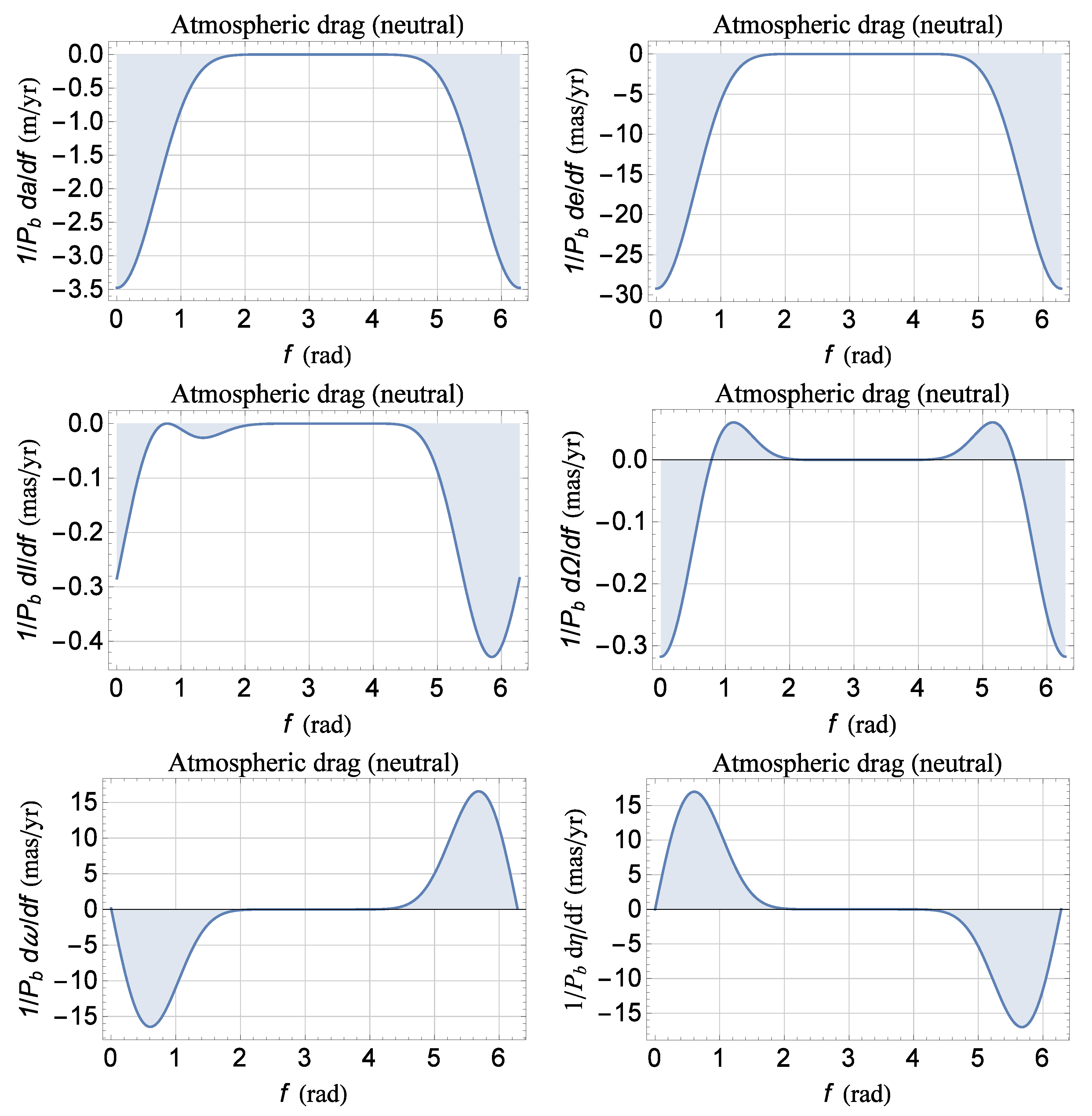
Figure A1.
Plots of Equations (A49) and (A54) as functions of the true anomaly f from 0 to 2π for the orbital configuration of Table A2. For the satellite, assumed spherical in shape and passive, we adopted as for the existing LARES [53]. In regard to the Earth’s atmospheric density, we adopted . Neither approximations in e nor in were used. The areas of the regions delimited by the curves and the f axis are the rates of change of the orbital elements averaged over one orbital period ; they are numerically calculated and displayed in Table A5. The value of was kept fixed over one orbital revolution.

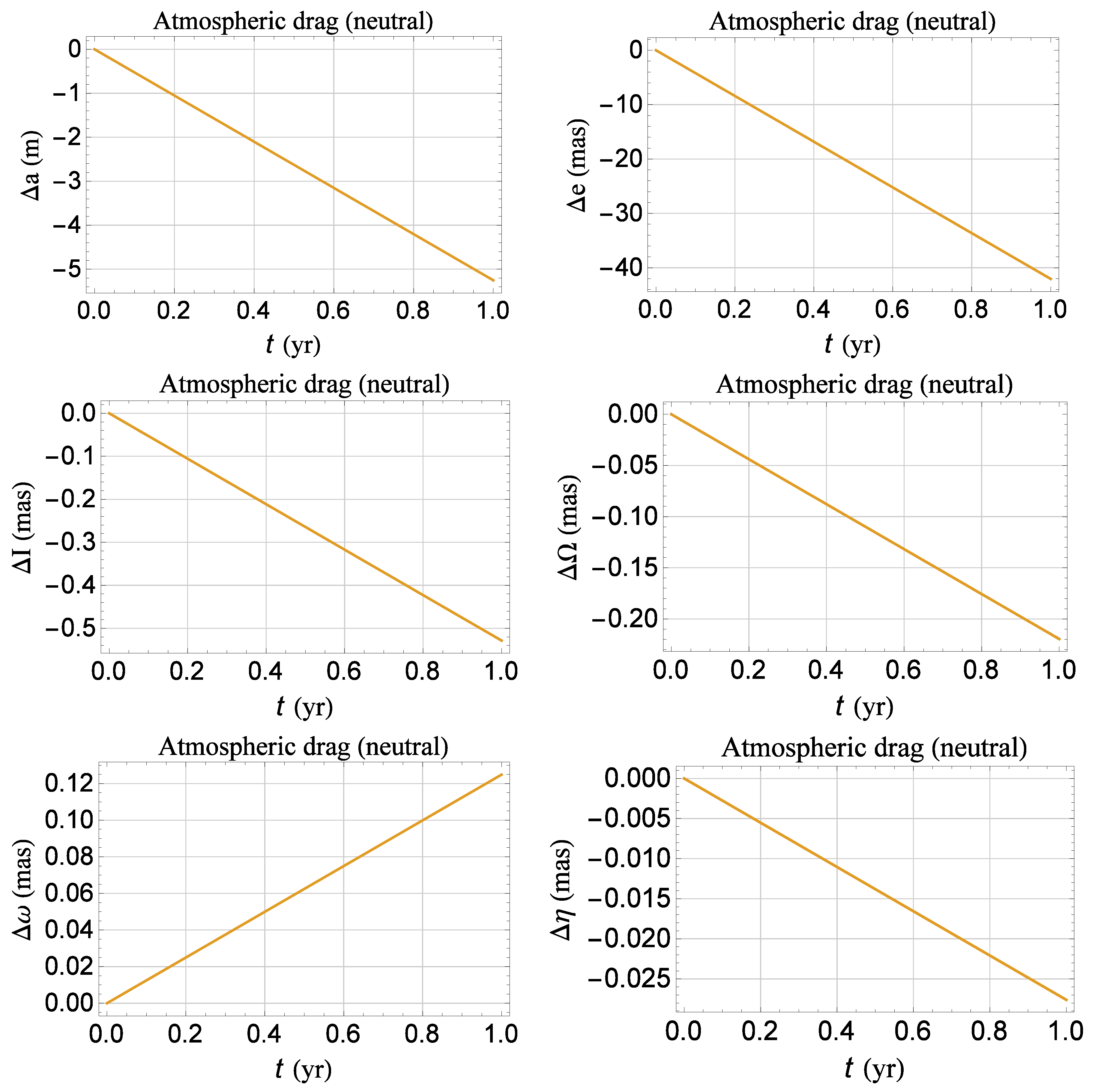
Figure A2.
Numerically integrated shifts of the semimajor axis a, the eccentricity e, the longitude of the ascending node , the argument of the perigee , and the mean anomaly at epoch for the orbital configuration of Table A2. For the satellite, assumed spherical in shape and passive, we adopted as for the existing LARES [53]. In regard to the Earth’s atmospheric density, we adopted . Cfr. with the semi-analytical results of Figure A1 and Table A5.

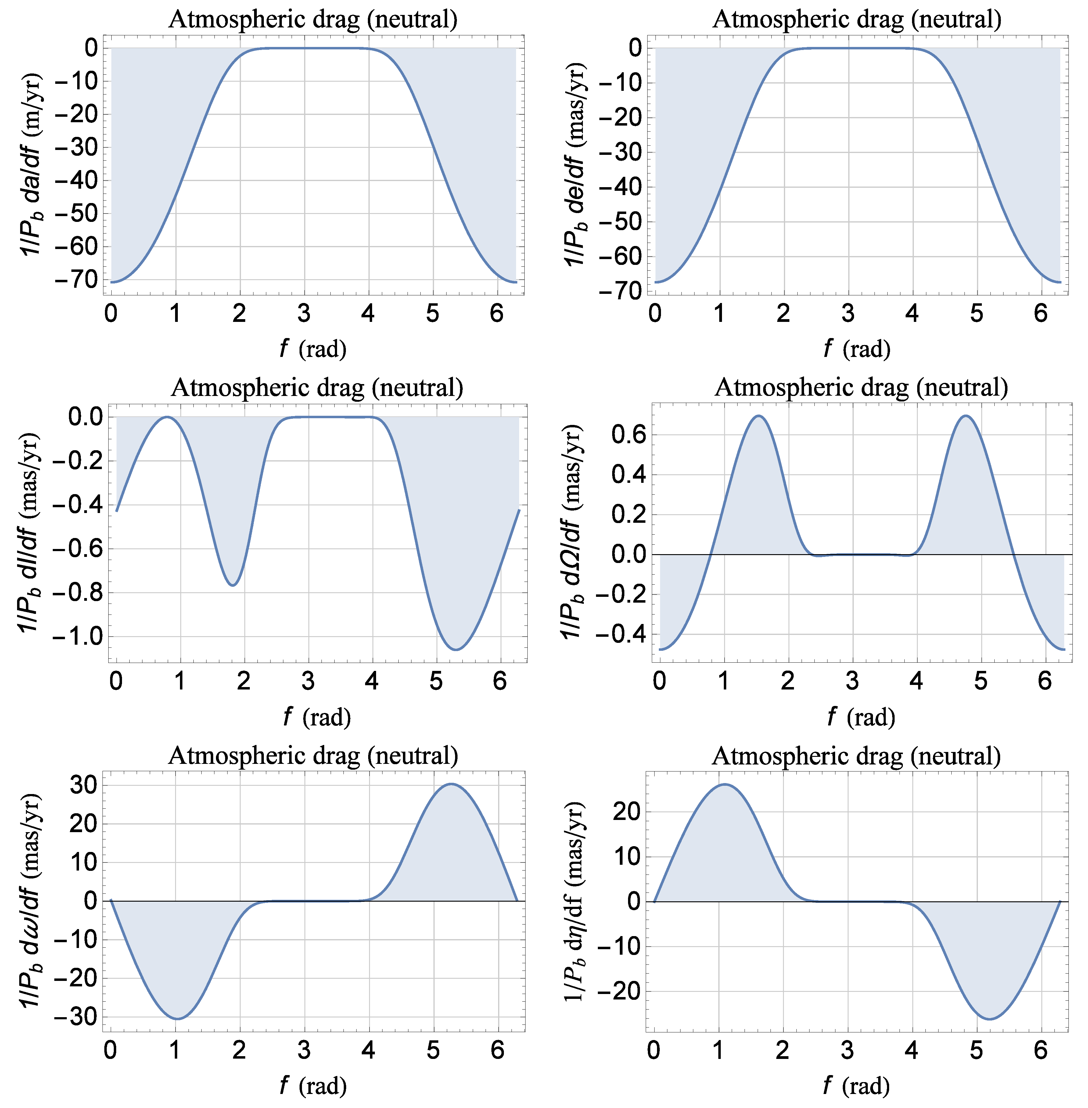
Figure A3.
Plots of Equations (A49) and (A54) as functions of the true anomaly f from 0 to 2π for the orbital configuration of Table A6. For the satellite, assumed spherical in shape and passive, we adopted as for the existing LARES [53]. In regard to the Earth’s atmospheric density, we adopted . Neither approximations in e nor in were used. The areas of the regions delimited by the curves and the f axis are the rates of change of the orbital elements averaged over one orbital period ; they are numerically calculated and displayed in Table A9. The value of was kept fixed over one orbital revolution.

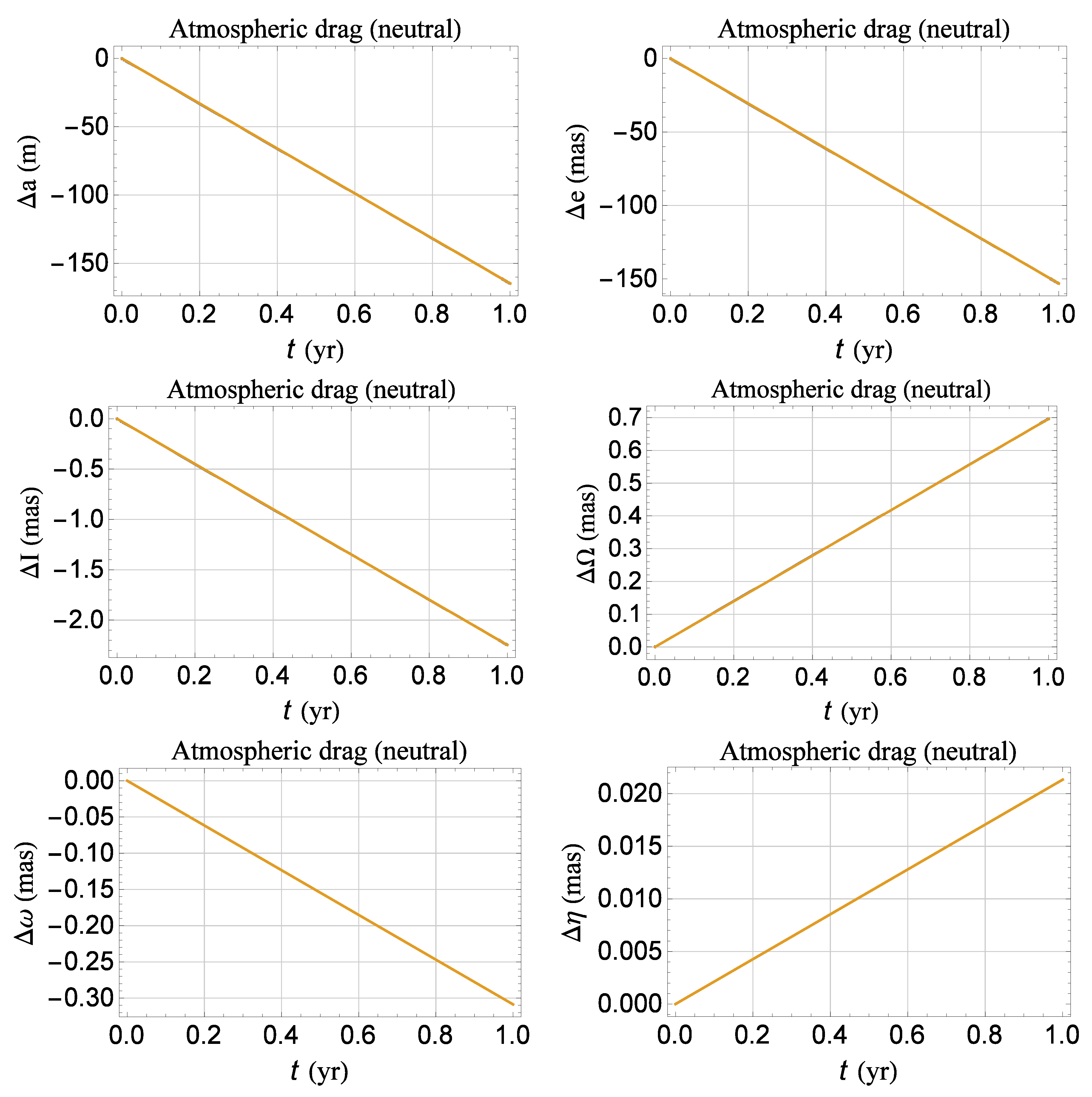
Figure A4.
Numerically integrated shifts of the semimajor axis a, the eccentricity e, the longitude of the ascending node , the argument of the perigee , and the mean anomaly at epoch for the orbital configuration of Table A6. For the satellite, assumed spherical in shape and passive, we adopted as for the existing LARES [53]. In regard to the Earth’s atmospheric density, we adopted . Cfr. with the semi-analytical results of Figure A3 and Table A9.

Appendix B. Classical Long-Term Rates of Change of the Keplerian Orbital Elements up to Degree ℓ = 8
Here, we will analytically work out the coefficients of the long-term rates of change of the eccentricity e, the inclination I, the longitude of the ascending node , the argument of perigee , and the mean anomaly at epoch induced by the first seven zonal harmonics of the geopotential up to degree ; the averaged rates of change of the semimajor axis a are all vanishing. We will adopt the Lagrange planetary equations [55,56,57,58] applied to the perturbing potential of degree ℓ
where is the Legendre polynomial of degree ℓ, averaged over one orbital period as disturbing function. We will not make any a-priory assumption on the orbital configuration of the satellite. As far as the orientation of the Earth’s spin axis, we will align it to the reference z axis of an equatorial coordinate system. The following formulas include both the genuine secular and the harmonic components with the frequency of the perigee and its integer multiples.
Appendix B.1. The Eccentricity
Appendix B.2. The Inclination
Appendix B.3. The Longitude of the Ascending Node
Appendix B.4. The Argument of Perigee
Appendix B.5. The Mean Anomaly at Epoch
Appendix C. The Atmospheric Drag
The neutral and charged atmospheric drag is potentially a major source of systematic uncertainty since it induces long-term effects on all the satellite’s orbital elements which, for a frozen perigee configuration, may look like secular trends on which the time variability of the atmospheric density is superimposed.
For the sake of simplicity, we will model HERO as a cannonball, passive satellite with the same physical properties of the existing LARES satellite in order to make some quantitative estimates of the disturbing impact of the atmospheric drag on the pN effects of interest. Thus, its perturbing acceleration is customarily modeled as
where are the dimensionless drag coefficient of the spacecraft, its area-to-mass ratio, the atmospheric density at its height, and its velocity with respect to the atmosphere, respectively. By assuming that the atmosphere co-rotates with the Earth, can be posed equal to
where is the Earth’s angular velocity. In fact, a decrease of the co-rotation with the height is expected. Membrado & Pacheco [59] modeled it in two scenarios involving a constant and non-constant viscosity. In the first case, the second term in Equation (A38) must be rescaled by . In general, the atmospheric density may not be considered as constant throughout a highly eccentric orbit covering a wide range of geocentric distances, as in our case; thus, we will model it as
where is the atmospheric density at some reference distance , while is the characteristic scale length. By assuming
if the atmospheric density is known at the perigee and apogee heights, can be determined as
where
In the case of the orbital configuration of Table A2, the perigee height is ; we will determine the corresponding neutral atmospheric density as follows. The neutral atmospheric density at the LARES height, which is , amounts to [53]. According to Brito, Celestino & Moraes [60], the neutral atmospheric density at is (TD-88 model), or (NASA model). Thus, it is possible to calculate the characteristic scale length valid for the range as
depending on the value adopted for at . Since for the orbital configuration of HERO of Table A2 it is , one can determine by using just Equation (A44) in
depending on the value of adopted. As far as is concerned, since 13,169.9 is much larger than the height of, say, the LAGEOS satellite (), for which it is [54], it does not seem unreasonable to assume
or so. Thus, Equation (A41), applied to , given by Equation (A45), and , given by Equation (A46), allows to infer the value for which must be used in the calculation of the drag effect for HERO. It is
depending on the value of adopted. As far as the more eccentric orbital configuration of Table A6 is concerned, by adopting for the two possible values of and, say, , it turns out that
Actually, even the density at a given height may not be regarded as truly constant because of a variety of geophysical phenomena characterized by quite different time scales. Anyway, in order to have an order-of-magnitude evaluation of the perturbing action of Equation (A37) on the motion of HERO, we calculate the averaged rates of change of its Keplerian orbital elements by keeping in Equation (A39) fixed during one orbital period ; given its short duration, at least in the case of Table A2, it is not an unreasonable assumption. The large value of the eccentricity makes most of the existing results in the literature unsuitable to the present case; moreover, an exact analytical calculation without recurring to any approximation in both e and is difficult. Thus, we follow two complementary approaches. In one of them, we, first, plot in Figure A1 and Figure A3 the analytical expressions of the ratios of the right-hand-sides of the Gauss perturbing equations for the rates of change of the Keplerian orbital elements, evaluated onto the unperturbed Keplerian ellipse, to as functions of the true anomaly f. In the most general case, by assuming the co-rotation of the atmosphere, they are
where
and
is the argument of latitude. It is worthwhile noticing that, in general,
being even possible that
for some values of f, thus preventing from expanding it in powers of . Then, we numerically calculate the areas under the resulting curves, i.e., we numerically integrate the averaged rates of change of the orbital elements for the given orbital configuration: see Table A5 and Table A9. In the second approach, we numerically integrate the equations of motion of the satellite in rectangular Cartesian coordinates, referred to a geocentric equatorial coordinate system, with and without Equation (A37) over 1 year; both the runs share the same initial conditions. Then, we subtract the resulting time series of the orbital elements in order to single out their shifts due to the disturbing acceleration. Finally, we perform a linear fit of them, and look at their slopes; we plot the fitted trends as functions of time t in Figure A2 and Figure A4. Both the methods reciprocally agree well, as shown by Figure A1, Figure A2, Figure A3 and Figure A4 for the neutral drag. A slight reduction turns out to occur if the decrease of the atmospheric co-rotation with height is taken into account as modeled by Membrado & Pacheco [59] by assuming the simpler case of a constant viscosity. We tested our approach by checking that it was able to reproduce the observed features of the semimajor axis decay of LARES recently determined in Pardini et al. [53]. However, it must be stressed that such findings should be deemed just as indicative of the limitations of the scenario considered if a passive spacecraft were to be adopted. Indeed, they were computed preliminarily by assuming the same physical properties of the existing LARES satellite which, in principle, could well be superseded by a new, specifically manufactured spacecraft able to reduce both the drag coefficient and the area-to-mass ratio . Moreover, also the actual temporal variability of the atmospheric density over timescales larger than the satellite’s orbital period should be taken into account, especially if data will be collected during temporal intervals several years long. To this aim, it is important to note that an inspection of Equations (A49) and (A54) shows that no other sources of long-term modulation are present. Indeed, the circulating node does not enter them, contrary to the perigee which, however, is held fixed by the adopted value of the inclination I.
References
- Brumberg, V.A. Essential Relativistic Celestial Mechanics; Adam Hilger: Bristol, UK, 1991. [Google Scholar]
- Meichsner, J.; Soffel, M.H. Effects on satellite orbits in the gravitational field of an axisymmetric central body with a mass monopole and arbitrary spin multipole moments. Celest. Mech. Dyn. Astr. 2015, 123, 1. [Google Scholar] [CrossRef][Green Version]
- Soffel, M.H. Relativity in Astrometry, Celestial Mechanics and Geodesy; Springer: Heidelberg, Germany, 1989. [Google Scholar]
- Will, C.M. Incorporating post-Newtonian effects in -body dynamics. Phys. Rev. D 2014, 89, 044043. [Google Scholar] [CrossRef]
- Panhans, M.; Soffel, M.H. Gravito-magnetism of an extended celestial body. Class. Quantum Gravity 2014, 31, 245012. [Google Scholar] [CrossRef]
- Soffel, M.; Wirrer, R.; Schastok, J.; Ruder, H.; Schneider, M. Relativistic effects in the motion of artificial satellites: The oblateness of the central body I. Celest. Mech. Dyn. Astr. 1987, 42, 81. [Google Scholar] [CrossRef]
- Le Verrier, U.; de Lettre, M.; Le Verrier à, M. Faye sur la théorie de Mercure et sur le mouvement du périhélie de cette planète. Cr. Hebd. Acad. Sci. 1859, 49, 379. [Google Scholar]
- Einstein, A. Erklärung der Perihelbewegung des Merkur aus der allgemeinen Relativitätstheorie. Sitzungsberichte der Preußischen Akademie der Wissenschaften 1915, 47, 831–839. [Google Scholar]
- Shapiro, I.I. General Relativity and Gravitation; Ashby, N., Bartlett, D.F., Wyss, W., Eds.; Cambridge University Press: Cambridge, UK, 1990; pp. 313–330. [Google Scholar]
- Shapiro, I.I.; Pettengill, G.H.; Ash, M.E.; Ingalls, R.P.; Campbell, D.B.; Dyce, R.B. Mercury’s perihelion advance: determination by radar. Phys. Rev. Lett. 1972, 28, 1594. [Google Scholar] [CrossRef]
- Anderson, J.D.; Campbell, J.K.; Jurgens, R.F.; Lau, E.L.; Newhall, X.X.; Slade, M.A., III; Standish, E.M., Jr. Recent developments in Solar system tests of general relativity. In Proceedings of the Sixth Marcel Grossmann Meeting on General Relativity; Satō, F., Nakamura, T., Eds.; World Scientific: Singapore, 1992; pp. 353–355. [Google Scholar]
- Anderson, J.D.; Keesey, M.S.W.; Lau, E.L.; Standish, E.M., Jr.; Newhall, X.X. Tests of general relativity using astrometric and radio metric observations of the planets. Acta Astronaut. 1978, 5, 43–61. [Google Scholar] [CrossRef]
- Shapiro, I.I.; Ash, M.E.; Smith, W.B. Icarus: further confirmation of the relativistic perihelion precession. Phys. Rev. Lett. 1968, 20, 1517. [Google Scholar] [CrossRef]
- Shapiro, I.I.; Smith, W.B.; Ash, M.E.; Herrick, S. General relativity and the orbit of Icarus. Astron. J. 1971, 76, 588. [Google Scholar] [CrossRef]
- Kramer, M.; Stairs, I.H.; Manchester, R.N.; McLaughlin, M.A.; Lyne, A.G.; Ferdman, R.D.; Burgay, M.; Lorimer, D.R.; Possenti, A.; D’Amico, N.; et al. Tests of general relativity from timing the double pulsar. Science 2006, 314, 97. [Google Scholar] [CrossRef] [PubMed]
- Lucchesi, D.M.; Peron, R. Accurate measurement in the field of the earth of the general-relativistic precession of the LAGEOS II pericenter and new constraints on non-newtonian gravity. Phys. Rev. Lett. 2010, 105, 231103. [Google Scholar] [CrossRef] [PubMed]
- Lucchesi, D.M.; Peron, R. LAGEOS II pericenter general relativistic precession (1993–2005): Error budget and constraints in gravitational physics. Phys. Rev. D 2014, 89, 082002. [Google Scholar] [CrossRef]
- Lense, J.; Thirring, H. Über den Einfluss der Eigenrotation der Zentralkörper auf die Bewegung der Planeten und Monde nach der Einsteinschen Gravitationstheorie. Phys. Z. 1918, 19, 156. [Google Scholar]
- Pfister, H. On the history of the so-called Lense-Thirring effect. Gen. Relativ. Gravit. 2007, 39, 1735. [Google Scholar] [CrossRef]
- Pfister, H. Eleventh Marcel Grossmann Meeting on Recent Developments in Theoretical and Experimental General Relativity, Gravitation and Relativistic Field Theories; Kleinert, H., Jantzen, R.T., Ruffini, R., Eds.; World Scientific: Singapore, 2008; pp. 2456–2458. [Google Scholar]
- Pfister, H. Editorial note to: Hans Thirring, On the formal analogy between the basic electromagnetic equations and Einstein’s gravity equations in first approximation. Gen. Relativ. Gravit. 2012, 44, 3217. [Google Scholar] [CrossRef]
- Pfister, H. Relativity and Gravitation; Springer Proceedings in Physics; Bičák, J., Ledvinka, T., Eds.; Springer: Berlin/Heidelberg, Germany, 2014; Volume 157, pp. 191–197. [Google Scholar]
- Renzetti, G. History of the attempts to measure orbital frame-dragging with artificial satellites. Open Phys. 2013, 11, 531–544. [Google Scholar] [CrossRef]
- Lucchesi, D.M.; Anselmo, L.; Bassan, M.; Magnafico, C.; Pardini, C.; Peron, R.; Pucacco, G.; Visco, M. General Relativity Measurements in the Field of Earth with Laser-Ranged Satellites: State of the Art and Perspectives. Universe 2019, 5, 141. [Google Scholar] [CrossRef]
- Pugh, G. Proposal for a Satellite Test of the Coriolis Prediction of General Relativity; Research Memorandum 11, Weapons Systems Evaluation Group; The Pentagon: Washington, DC, USA, 1959. [Google Scholar]
- Schiff, L. Gravity probe B: final results of a space experiment to test general relativity. Phys. Rev. Lett. 1960, 4, 215. [Google Scholar] [CrossRef]
- Everitt, C.W.F.; DeBra, D.B.; Parkinson, B.W.; Turneaure, J.P.; Conklin, J.W.; Heifetz, M.I.; Keiser, G.M.; Silbergleit, A.S.; Holmes, T.; Kolodziejczak, J.; et al. Gravity probe B: final results of a space experiment to test general relativity. Phys. Rev. Lett. 2011, 106, 221101. [Google Scholar] [CrossRef]
- Everitt, C.W.F.; Muhlfelder, B.; DeBra, D.B.; Parkinson, B.W.; Turneaure, J.P.; Silbergleit, A.S.; Acworth, E.B.; Adams, M.; Adler, R.; Bencze, W.J.; et al. The Gravity Probe B test of general relativity. Class. Quantum Gravity 2015, 32, 224001. [Google Scholar] [CrossRef]
- Everitt, C.W.F.; Buchman, S.; Debra, D.B.; Keiser, G.M.; Lockhart, J.M.; Muhlfelder, B.; Parkinson, B.W.; Turneaure, J.P. Gyros, Clocks, Interferometers …: Testing Relativistic Gravity in Space. In Lecture Notes in Physics; Lämmerzahl, C., Everitt, C.W.F., Hehl, F.W., Eds.; Springer: Berlin, Germany, 2001; Volume 562, p. 52. [Google Scholar]
- Iorio, L. Post-Newtonian direct and mixed orbital effects due to the oblateness of the central body. Int. J. Mod. Phys. D 2015, 24, 1550067. [Google Scholar] [CrossRef]
- Iorio, L. The post-Newtonian gravitomagnetic spin-octupole moment of an oblate rotating body and its effects on an orbiting test particle; are they measurable in the Solar system? Mon. Not. R. Astron. Soc. 2019, 484, 4811. [Google Scholar] [CrossRef]
- Iorio, L. A possible new test of general relativity with Juno. Class. Quantum Gravity 2013, 30, 195011. [Google Scholar] [CrossRef]
- Abbas, U.; Bucciarelli, B.; Lattanzi, M.G. Differential astrometric framework for the Jupiter relativistic experiment with Gaia. Mon. Not. Roy. Astron. Soc. 2019, 485, 1147. [Google Scholar] [CrossRef]
- Crosta, M.T.; Mignard, F. Microarcsecond light bending by Jupiter. Class. Quantum Gravity 2006, 23, 4853. [Google Scholar] [CrossRef][Green Version]
- Kopeikin, S.M.; Makarov, V.V. Gravitational bending of light by planetary multipoles and its measurement with microarcsecond astronomical interferometers. Phys. Rev. D 2007, 75, 062002. [Google Scholar] [CrossRef]
- Le Poncin-Lafitte, C.; Teyssandier, P. Influence of mass multipole moments on the deflection of a light ray by an isolated axisymmetric body. Phys. Rev. D 2008, 77, 044029. [Google Scholar] [CrossRef]
- Angélil, R.; Saha, P.; Bondarescu, R.; Jetzer, P.; Schärer, A.; Lundgren, A. Spacecraft clocks and relativity: Prospects for future satellite missions. Phys. Rev. D 2014, 89, 064067. [Google Scholar] [CrossRef]
- Schärer, A.; Angélil, R.; Bondarescu, R.; Jetzer, P.; Lundgren, A. Testing scalar-tensor theories and parametrized post-Newtonian parameters in Earth orbit. Phys. Rev. D 2014, 90, 123005. [Google Scholar] [CrossRef]
- Schärer, A.; Bondarescu, R.; Saha, P.; Angélil, R.; Helled, R.; Jetzer, P. Prospects for Measuring Planetary Spin and Frame-Dragging in Spacecraft Timing Signals. Front. Astron. Space Sci. 2017, 4, 11. [Google Scholar] [CrossRef]
- Delva, P.; Puchades, N.; Schönemann, E.; Dilssner, F.; Courde, C.; Bertone, S.; Gonzalez, F.; Hees, A.; Le Poncin-Lafitte, C.; Meynadier, F.; et al. Gravitational Redshift Test Using Eccentric Galileo Satellites. Phys. Rev. Lett. 2018, 121, 231101. [Google Scholar] [CrossRef] [PubMed]
- Herrmann, S.; Finke, F.; Lülf, M.; Kichakova, O.; Puetzfeld, D.; Knickmann, D.; List, M.; Rievers, B.; Giorgi, G.; Günther, C.; et al. Test of the Gravitational Redshift with Galileo Satellites in an Eccentric Orbit. Phys. Rev. Lett. 2018, 121, 231102. [Google Scholar] [CrossRef] [PubMed]
- Altschul, B.; Bailey, Q.G.; Blanchet, L.; Bongs, K.; Bouyer, P.; Cacciapuoti, L.; Capozziello, S.; Gaaloul, N.; Giulini, D.; Hartwi, J.; et al. Quantum tests of the Einstein Equivalence Principle with the STE–QUEST space mission. Adv. Space Res. 2015, 55, 501. [Google Scholar] [CrossRef]
- Clifton, T.; Ferreira, P.G.; Padilla, A.; Skordis, C. Modified gravity and cosmology. Phys. Rep. 2012, 513, 1. [Google Scholar] [CrossRef]
- Rubincam, D.P. On the secular decrease in the semimajor axis of LAGEOS’s orbit. Celest. Mech. Dyn. Astr. 1982, 26, 361. [Google Scholar] [CrossRef]
- Sośnica, K. Determination of Precise Satellite Orbits and Geodetic Parameters Using Satellite Laser Ranging; ETH Zürich, Swiss Geodetic Commission: Zürich, Switzerland, 2014; pp. 94–95. [Google Scholar]
- Sośnica, K.; Baumann, C.; Thaller, D.; Jäggi, A.; Dach, R. Combined LARES-LAGEOS Solutions. In Proceedings of the 18th International Workshop on Laser Ranging, Fujiyoshida, Japan, 11–15 November 2013. 13-Po-57. [Google Scholar]
- Ciufolini, I.; Lucchesi, D.; Vespe, F.; Mandiello, A. Measurement of dragging of inertial frames and gravitomagnetic field using laser-ranged satellites. Nuovo Cimento A 1996, 109, 575. [Google Scholar] [CrossRef]
- Chen, Q.; Shen, Y.; Francis, O.; Chen, W.; Zhang, X.; Hsu, H.J. Tongji-Grace02s and Tongji-Grace02k: High-Precision Static GRACE-Only Global Earth’s Gravity Field Models Derived by Refined Data Processing Strategies. Geophys. Res. 2018, 123, 6111. [Google Scholar] [CrossRef]
- Sheard, B.S.; Heinzel, G.; Danzmann, K.; Shaddock, D.A.; Klipstein, W.M.; Folkner, W.M.J. Intersatellite laser ranging instrument for the GRACE follow-on mission. Geodesy 2012, 86, 1083. [Google Scholar] [CrossRef]
- Sehnal, L. Effects of the terrestrial infrared radiation pressure on the motion of an artificial satellite. Celest. Mech. Dyn. Astr. 1981, 25, 169. [Google Scholar] [CrossRef]
- Durand-Manterola, H.J. Dipolar magnetic moment of the bodies of the solar system and the Hot Jupiters. Planet. Space Sci. 2009, 57, 1405. [Google Scholar] [CrossRef][Green Version]
- Petit, G.; Luzum, B. IERS Conventions (2010). IERS Techn. Note 2010, 36, 1. [Google Scholar]
- Pardini, C.; Anselmo, L.; Lucchesi, D.M.; Peron, R. On the secular decay of the LARES semi-major axis. Acta Astronaut. 2017, 140, 469. [Google Scholar] [CrossRef]
- Lucchesi, D.M.; Anselmo, L.; Bassan, M.; Pardini, C.; Peron, R.; Pucacco, G.; Visco, M. Testing the gravitational interaction in the field of the Earth via satellite laser ranging and the Laser Ranged Satellites Experiment (LARASE). Class. Quantum Gravity 2015, 32, 155012. [Google Scholar] [CrossRef]
- Bertotti, B.; Farinella, P.; Vokrouhlický, D. Physics of the Solar System; Kluwer Academic Press: Dordrecht, The Netherlands, 2003. [Google Scholar]
- Capderou, M. Satellites: Orbits and Missions; Springer: Berlin, Germany, 2005. [Google Scholar]
- Kopeikin, S.; Efroimsky, M.; Kaplan, G. Relativistic Celestial Mechanics of the Solar System; Wiley-VCH: Weinheim, Germany, 2011. [Google Scholar]
- Xu, G. Orbits; Springer: Berlin, Germany, 2008. [Google Scholar]
- Membrado, M.; Pacheco, A.F. Decrease of the atmospheric co-rotation with height. Eur. J. Phys. 2010, 31, 1013. [Google Scholar] [CrossRef]
- Brito, T.P.; Celestino, C.C.; Moraes, R.V. Study of the decay time of a CubeSat type satellite considering perturbations due to the Earth’s oblateness and atmospheric drag. J. Phys. Conf. Ser. 2015, 641, 012026. [Google Scholar] [CrossRef]
| 1. | |
| 2. | In that case, the aliasing Newtonian effect which must be disentangled from the pN perihelion precessions is due to the quadrupole mass moment of the Sun. |
| 3. | |
| 4. | At least one of them must be affected by the pN effect one is looking for. In principle, the N orbital elements may be different from one another belonging to the same satellite, or some of them may be identical belonging to different spacecraft (e.g., the nodes of two different vehicles). |
| 5. | In general, it is not necessarily one of the parameters of the parameterized post-Newtonian (PPN) formalism, being possibly a combination of some of them. |
© 2019 by the author. Licensee MDPI, Basel, Switzerland. This article is an open access article distributed under the terms and conditions of the Creative Commons Attribution (CC BY) license (http://creativecommons.org/licenses/by/4.0/).
Share and Cite
MDPI and ACS Style
Iorio, L. A HERO for General Relativity. Universe 2019, 5, 165. https://doi.org/10.3390/universe5070165
AMA Style
Iorio L. A HERO for General Relativity. Universe. 2019; 5(7):165. https://doi.org/10.3390/universe5070165
Chicago/Turabian StyleIorio, Lorenzo. 2019. "A HERO for General Relativity" Universe 5, no. 7: 165. https://doi.org/10.3390/universe5070165
APA StyleIorio, L. (2019). A HERO for General Relativity. Universe, 5(7), 165. https://doi.org/10.3390/universe5070165
Note that from the first issue of 2016, this journal uses article numbers instead of page numbers. See further details here.